A Quantitative Analysis of the Ignition Characteristics
of Fine Iron Particles

Microscopic cross-section views of a solid-phase oxide scale grown on iron under isothermal conditions (over a range in temperature from $973~\mathrm{K}$ to $1523~\mathrm{K}$) in air were first obtained by Païdassi in the 1950s [Paidassi1958a]. Figure 1(a) is a sample image from Ref. [Paidassi1958a] showing that an iron-oxide scale consists of three compact layers of hematite ($\text{Fe}{\vphantom{\text{X}}}_{\smash[t]{\text{2}}}\text{O}{\vphantom{\text{X}}}_{\smash[t]{\text{3}}}$), magnetite ($\text{Fe}{\vphantom{\text{X}}}_{\smash[t]{\text{3}}}\text{O}{\vphantom{\text{X}}}_{\smash[t]{\text{4}}}$), and wüstite (FeO) stacked from the gas-oxide interface to the oxide-iron interface. The relative thicknesses of the $\text{Fe}{\vphantom{\text{X}}}_{\smash[t]{\text{2}}}\text{O}{\vphantom{\text{X}}}_{\smash[t]{\text{3}}}$, $\text{Fe}{\vphantom{\text{X}}}_{\smash[t]{\text{3}}}\text{O}{\vphantom{\text{X}}}_{\smash[t]{\text{4}}}$, and FeO layers with respect to the total thickness of the oxide scale are $1\%$, $4\%$, and $95\%$, respectively. As conceptually illustrated in Fig. 1(b), for a compact oxide film (i.e., without cracks or grain boundaries to facilitate oxygen transport to the iron core), solid-phase iron oxidation consists of the following processes:

1. 1.

   Diffusion of oxygen ($\text{O}{\vphantom{\text{X}}}_{\smash[t]{\text{2}}}$) molecules from the bulk gas to the gas-oxide interface.

2. 2.

   Incorporation of oxygen into the oxide scale (i.e., a dissociative absorption of $\text{O}{\vphantom{\text{X}}}_{\smash[t]{\text{2}}}$ molecules as oxygen anions $\text{O}{\vphantom{\text{X}}}^{\text{2\hskip 0.81375pt--\hskip 0.81375pt}}$).

3. 3.

   Absorption of iron into the oxide film as iron cations.

4. 4.

   Diffusion of ions and electrons through the oxide scale.

5. 5.

   Reactions at FeO-$\text{Fe}{\vphantom{\text{X}}}_{\smash[t]{\text{3}}}\text{O}{\vphantom{\text{X}}}_{\smash[t]{\text{4}}}$, $\text{Fe}{\vphantom{\text{X}}}_{\smash[t]{\text{3}}}\text{O}{\vphantom{\text{X}}}_{\smash[t]{\text{4}}}$-$\text{Fe}{\vphantom{\text{X}}}_{\smash[t]{\text{2}}}\text{O}{\vphantom{\text{X}}}_{\smash[t]{\text{3}}}$, and $\text{Fe}{\vphantom{\text{X}}}_{\smash[t]{\text{2}}}\text{O}{\vphantom{\text{X}}}_{\smash[t]{\text{3}}}$-$\text{O}{\vphantom{\text{X}}}_{\smash[t]{\text{2}}}$ interfaces.

At relatively low temperatures, the diffusion of oxygen in the gas phase (Process 1) is much more rapid than the kinetic processes (2 to 5) in the solid phase. As the temperature of the particle increases, the solid-phase kinetics become increasingly rapid, and thus, the external diffusion of oxygen becomes the rate-limiting process. In this analysis, the oxidation rate is considered to be only controlled by the solid-phase kinetics for determining the critical conditions for particle ignition, i.e., the critical temperature required to trigger thermal runaway, in Sects. 5.1-5.5; a switch-type reaction-rate model, considering the transition from kinetic- to external-diffusion-controlled combustion, is used describe the ignition behavior of iron particles beyond the critical temperature for thermal runaway, in Sects. 5.6 and 5.7.

For a sufficiently thick oxide scale, the growth rate of each layer is controlled by the diffusion of ions subjected to the equilibrium activities of Fe and O at the interfaces [ChenYuen2003]. Considering the fact that the transport of electrons and the establishment of local equilibria at the interfaces are significantly more rapid than the diffusion of ions across the oxide layers, Wagner’s theory [Wagner1933] relates the oxide growth rate to the diffusivity of ions. Since Fe cations are significantly more mobile in FeO and $\text{Fe}{\vphantom{\text{X}}}_{\smash[t]{\text{3}}}\text{O}{\vphantom{\text{X}}}_{\smash[t]{\text{4}}}$ layers than O anions due to a large size of O anion ($1.4~\mathrm{\AA}$) [Li2011EnergyEnviron], the growth of oxide film is predominantly governed by the outward diffusion of Fe cations [Himmel1953JOM, SmeltzerYoung1975]. The growth of the FeO layer is the most rapid due to the fact that the diffusion coefficient of Fe cations in FeO is greater than that in $\text{Fe}{\vphantom{\text{X}}}_{\smash[t]{\text{3}}}\text{O}{\vphantom{\text{X}}}_{\smash[t]{\text{4}}}$ or $\text{Fe}{\vphantom{\text{X}}}_{\smash[t]{\text{2}}}\text{O}{\vphantom{\text{X}}}_{\smash[t]{\text{3}}}$. Such a diffusion-controlled growth follows a parabolic rate law,

$$\frac{\mathrm{d}X_{i}}{\mathrm{d}t}=\frac{k_{\mathrm{p},i}}{X_{i}}$$

(1)

where $X_{i}$ is the thickness of an oxide layer, $k_{\mathrm{p},i}$ is the parabolic rate constant, and $i$ is the index of each oxide layer. Yurek et al. [Yurek1974] and Garnaud and Rapp [GarnaudRapp1977] extended Wagner’s theory to show that the growth of a multilayered oxide film on iron follows a parabolic rate law governed by the diffusion coefficients of Fe in FeO and $\text{Fe}{\vphantom{\text{X}}}_{\smash[t]{\text{3}}}\text{O}{\vphantom{\text{X}}}_{\smash[t]{\text{4}}}$. It is of importance to note that, as revealed by Goursat and Smeltzer [Goursat1973kinetics], the oxidation kinetics of FeO is independent of ambient oxygen concentration over a temperature range (at least) from $1073~\mathrm{K}$ to $1273~\mathrm{K}$ for a partial pressure of $\text{O}{\vphantom{\text{X}}}_{\smash[t]{\text{2}}}$ ($p_{\mathrm{{}\mathrm{O}{\vphantom{\mathrm{X}}}_{\smash[t]{\mathrm{2}}}}}$) above $4\times 10^{-4}~\mathrm{atm}$. As the activities of Fe and O at the Fe-FeO, FeO-$\text{Fe}{\vphantom{\text{X}}}_{\smash[t]{\text{3}}}\text{O}{\vphantom{\text{X}}}_{\smash[t]{\text{4}}}$, and $\text{Fe}{\vphantom{\text{X}}}_{\smash[t]{\text{3}}}\text{O}{\vphantom{\text{X}}}_{\smash[t]{\text{4}}}$-$\text{Fe}{\vphantom{\text{X}}}_{\smash[t]{\text{2}}}\text{O}{\vphantom{\text{X}}}_{\smash[t]{\text{3}}}$ interfaces are fixed by the phase equilibria, the growth of FeO and $\text{Fe}{\vphantom{\text{X}}}_{\smash[t]{\text{3}}}\text{O}{\vphantom{\text{X}}}_{\smash[t]{\text{4}}}$ are barely affected by the ambient $\text{O}{\vphantom{\text{X}}}_{\smash[t]{\text{2}}}$ concentration [Young2008]. In this analysis, the kinetic rates of FeO and $\text{Fe}{\vphantom{\text{X}}}_{\smash[t]{\text{3}}}\text{O}{\vphantom{\text{X}}}_{\smash[t]{\text{4}}}$ formation are assumed to be independent of ambient $\text{O}{\vphantom{\text{X}}}_{\smash[t]{\text{2}}}$ concentration as long as $p_{\mathrm{{}\mathrm{O}{\vphantom{\mathrm{X}}}_{\smash[t]{\mathrm{2}}}}}$ is greater than zero. The implication of this assumption on the ignition process—the transition from a kinetic-controlled combustion to an $\text{O}{\vphantom{\text{X}}}_{\smash[t]{\text{2}}}$-diffusion-controlled (also referred to as external-diffusion-controlled) combustion—of an iron particle is discussed in Sect. 5.6.

Since the growth of the $\text{Fe}{\vphantom{\text{X}}}_{\smash[t]{\text{2}}}\text{O}{\vphantom{\text{X}}}_{\smash[t]{\text{3}}}$ layer is significantly slower in comparison to the growth of the FeO and $\text{Fe}{\vphantom{\text{X}}}_{\smash[t]{\text{3}}}\text{O}{\vphantom{\text{X}}}_{\smash[t]{\text{4}}}$ layers, the energy release due to the formation $\text{Fe}{\vphantom{\text{X}}}_{\smash[t]{\text{2}}}\text{O}{\vphantom{\text{X}}}_{\smash[t]{\text{3}}}$ is negligible. The formation of this thin $\text{Fe}{\vphantom{\text{X}}}_{\smash[t]{\text{2}}}\text{O}{\vphantom{\text{X}}}_{\smash[t]{\text{3}}}$ layer is thus neglected in the current analysis. It is, however, of importance to understand the role played by the hematite layer on the formation of the inner oxidized layers. There is experimental evidence [Kofstad1972, Atkinson1985] indicating that the formation of $\text{Fe}{\vphantom{\text{X}}}_{\smash[t]{\text{2}}}\text{O}{\vphantom{\text{X}}}_{\smash[t]{\text{3}}}$ is due to both an outward diffusion of Fe cations and an inward diffusion of O anions at comparable rates (as illustrated in Fig. 1(b)), possibly along cracks in the hematite layer. Goursat and Smeltzer [Goursat1973kinetics] showed that the $\text{Fe}{\vphantom{\text{X}}}_{\smash[t]{\text{2}}}\text{O}{\vphantom{\text{X}}}_{\smash[t]{\text{3}}}$ layer formed upon the $\text{Fe}{\vphantom{\text{X}}}_{\smash[t]{\text{3}}}\text{O}{\vphantom{\text{X}}}_{\smash[t]{\text{4}}}$ layer is a dense “forest” of whiskers and platelets. The growth rate of this irregular hematite layer adapts to the ambient $\text{O}{\vphantom{\text{X}}}_{\smash[t]{\text{2}}}$ concentration, establishing an equilibrium at the $\text{Fe}{\vphantom{\text{X}}}_{\smash[t]{\text{3}}}\text{O}{\vphantom{\text{X}}}_{\smash[t]{\text{4}}}$-$\text{Fe}{\vphantom{\text{X}}}_{\smash[t]{\text{3}}}\text{O}{\vphantom{\text{X}}}_{\smash[t]{\text{2}}}$ interface, and thus, making the growth rates of FeO and $\text{Fe}{\vphantom{\text{X}}}_{\smash[t]{\text{3}}}\text{O}{\vphantom{\text{X}}}_{\smash[t]{\text{4}}}$ independent of $\text{O}{\vphantom{\text{X}}}_{\smash[t]{\text{2}}}$ concentration.

The experimental data of Païdassi [Paidassi1958a] reveal that, at a steady temperature, the thickness of each oxide layer $X_{i}$ increases with square root of time $\sqrt{t}$ at a constant rate, indeed following a parabolic rate law. The parabolic rate constant $k_{i}$ can be measured as the slope of the fitted line to the experimental data of $X_{i}$ as a function of $\sqrt{t}$ at each temperature, i.e., $X_{i}=k_{i}\sqrt{t}+X_{i,0}$, as reported in Table 1 of Ref. [Paidassi1958a]. Note that $k_{i}$ can be converted to the rate constant $k_{\mathrm{p},i}$ in Eq. 1 via the relation as follows:

$$k_{\mathrm{p},i}=\frac{{k_{i}}^{2}}{2}$$

(2)

The natural logarithmic values of the experimental data of $k_{\mathrm{p},i}$ for the growth of total oxide film thickness (blue diamond), FeO layer thickness (red square), and $\text{Fe}{\vphantom{\text{X}}}_{\smash[t]{\text{3}}}\text{O}{\vphantom{\text{X}}}_{\smash[t]{\text{4}}}$ layer thickness (black circle) are plotted in Fig. 2 as a function of the reciprocal of temperature, $1/T$. These data points demonstrate a linear regression, i.e., the parabolic rate constant increases exponentially with temperature, indicating that the diffusion of Fe cations in the oxide layers is an activated process. The temperature dependence of $k_{\mathrm{p},i}$ can be described by an Arrhenius function as follows,

$$k_{\mathrm{p},i}(T)=k_{0,i}\mathrm{Exp}\left(\frac{-T_{\mathrm{a},i}}{T}\right)$$

(3)

wherein the values of pre-exponential factor $k_{0,i}$ and activation temperature $T_{\mathrm{a},i}$ for the growth of FeO and $\text{Fe}{\vphantom{\text{X}}}_{\smash[t]{\text{3}}}\text{O}{\vphantom{\text{X}}}_{\smash[t]{\text{4}}}$ layers can be calibrated via line fitting to the plotted data points as reported in Table 1.

This model considers a spherical particle consisting of a core of iron, an inner FeO layer, and an outer $\text{Fe}{\vphantom{\text{X}}}_{\smash[t]{\text{3}}}\text{O}{\vphantom{\text{X}}}_{\smash[t]{\text{4}}}$ layer as illustrated in Fig. 3(a). For the temperature range over which the oxidation kinetic model is calibrated, i.e., $973~\mathrm{K}$ to $1523~\mathrm{K}$, the thickness of $\text{Fe}{\vphantom{\text{X}}}_{\smash[t]{\text{2}}}\text{O}{\vphantom{\text{X}}}_{\smash[t]{\text{3}}}$ is about $1~\%$ of the total thickness of the oxide film. The formation of $\text{Fe}{\vphantom{\text{X}}}_{\smash[t]{\text{2}}}\text{O}{\vphantom{\text{X}}}_{\smash[t]{\text{3}}}$ is thus neglected in this model. Since the thermal conductivities of Fe and FeO are greater than that of the surrounding gas by two to three orders of magnitude, a typical Biot number of a fine iron particle is on the order of $0.001$-$0.01$. Hence, a uniform particle temperature, $T_{\mathrm{p}}$, can be assumed. The particle exchanges heat with the ambient gas at a temperature $T_{\mathrm{g}}$ via convective and radiative heat transfer. Other major assumptions on which the current model is based are summarized in the list below:

1. 1.

   The densities of solid iron, FeO, $\text{Fe}{\vphantom{\text{X}}}_{\smash[t]{\text{3}}}\text{O}{\vphantom{\text{X}}}_{\smash[t]{\text{4}}}$ are considered as constant values, i.e., the effect of thermal expansion is neglected. Given the fact that, in the temperature range between $900\text{\,}\mathrm{K}$ and $1200\text{\,}\mathrm{K}$, which is relevant to the current analysis, the coefficients of thermal expansion of Fe, FeO, and $\text{Fe}{\vphantom{\text{X}}}_{\smash[t]{\text{3}}}\text{O}{\vphantom{\text{X}}}_{\smash[t]{\text{4}}}$ vary over approximately the same range on the order of $1\times 10^{-6}\mathrm{K}^{-1}$ [Carter1959, Holcomb2019, Kozlovskii2019], oxide layer cracking due the mismatch in thermal expansion between the oxide shell and the metal core is unlikely to core for iron particles.

2. 2.

   The phase changes from $\alpha$-Fe to $\gamma$-Fe and from $\gamma$-Fe to $\delta$-Fe are not considered since the associated latent heats are much less than the specific energy release of FeO and $\text{Fe}{\vphantom{\text{X}}}_{\smash[t]{\text{3}}}\text{O}{\vphantom{\text{X}}}_{\smash[t]{\text{4}}}$ formation. The thermodynamic properties of iron used in the calculation are those of $\alpha$-Fe.

3. 3.

   Curvature effect on the oxide layer growth is neglected as the oxide layer thickness is much less than the particle radius during the ignition process.

4. 4.

   The flow velocity of the ambient gas relative to the particle is negligible, i.e., the corresponding Reynolds number is zero.

The mass balance equations for Fe, FeO, and $\text{Fe}{\vphantom{\text{X}}}_{\smash[t]{\text{3}}}\text{O}{\vphantom{\text{X}}}_{\smash[t]{\text{4}}}$ can be related to the parabolic kinetic model (Eqs. 1 and 3) as follows,

$$\frac{\mathrm{d}m_{{}\mathrm{Fe}}}{\mathrm{d}t}=-\nu_{{}\mathrm{Fe}/{}\mathrm{FeO}}\frac{\mathrm{d}m_{{}\mathrm{FeO}}}{\mathrm{d}t}-\nu_{{}\mathrm{Fe}/{}{}\mathrm{Fe}{\vphantom{\mathrm{X}}}_{\smash[t]{\mathrm{3}}}\mathrm{O}{\vphantom{\mathrm{X}}}_{\smash[t]{\mathrm{4}}}}\frac{\mathrm{d}m_{{}{}\mathrm{Fe}{\vphantom{\mathrm{X}}}_{\smash[t]{\mathrm{3}}}\mathrm{O}{\vphantom{\mathrm{X}}}_{\smash[t]{\mathrm{4}}}}}{\mathrm{d}t}$$

(4)

$$\frac{\mathrm{d}m_{{}\mathrm{FeO}}}{\mathrm{d}t}=\rho_{{}\mathrm{FeO}}A_{{}\mathrm{FeO}}\frac{\mathrm{d}X_{{}\mathrm{FeO}}}{\mathrm{d}t}=\frac{\rho_{{}\mathrm{FeO}}A_{{}\mathrm{FeO}}k_{0,{}\mathrm{FeO}}}{X_{{}\mathrm{FeO}}}\;\mathrm{Exp}\left(\frac{-T_{\mathrm{a,FeO}}}{T_{\mathrm{p}}}\right)$$

(5)

$$\frac{\mathrm{d}m_{{}{}\mathrm{Fe}{\vphantom{\mathrm{X}}}_{\smash[t]{\mathrm{3}}}\mathrm{O}{\vphantom{\mathrm{X}}}_{\smash[t]{\mathrm{4}}}}}{\mathrm{d}t}=\rho_{{}{}\mathrm{Fe}{\vphantom{\mathrm{X}}}_{\smash[t]{\mathrm{3}}}\mathrm{O}{\vphantom{\mathrm{X}}}_{\smash[t]{\mathrm{4}}}}A_{\mathrm{p}}\frac{\mathrm{d}X_{{}{}\mathrm{Fe}{\vphantom{\mathrm{X}}}_{\smash[t]{\mathrm{3}}}\mathrm{O}{\vphantom{\mathrm{X}}}_{\smash[t]{\mathrm{4}}}}}{\mathrm{d}t}=\frac{\rho_{{}{}\mathrm{Fe}{\vphantom{\mathrm{X}}}_{\smash[t]{\mathrm{3}}}\mathrm{O}{\vphantom{\mathrm{X}}}_{\smash[t]{\mathrm{4}}}}A_{\mathrm{p}}k_{0,{}{}\mathrm{Fe}{\vphantom{\mathrm{X}}}_{\smash[t]{\mathrm{3}}}\mathrm{O}{\vphantom{\mathrm{X}}}_{\smash[t]{\mathrm{4}}}}}{X_{{}{}\mathrm{Fe}{\vphantom{\mathrm{X}}}_{\smash[t]{\mathrm{3}}}\mathrm{O}{\vphantom{\mathrm{X}}}_{\smash[t]{\mathrm{4}}}}}\;\mathrm{Exp}\left(\frac{-T_{\mathrm{a,{}{}\mathrm{Fe}{\vphantom{\mathrm{X}}}_{\smash[t]{\mathrm{3}}}\mathrm{O}{\vphantom{\mathrm{X}}}_{\smash[t]{\mathrm{4}}}}}}{T_{\mathrm{p}}}\right)$$

(6)

where $\nu_{{}\mathrm{Fe}/{}\mathrm{FeO}}$ and $\nu_{{}\mathrm{Fe}/{}{}\mathrm{Fe}{\vphantom{\mathrm{X}}}_{\smash[t]{\mathrm{3}}}\mathrm{O}{\vphantom{\mathrm{X}}}_{\smash[t]{\mathrm{4}}}}$ are the stoichiometric mass ratios. Note that the formation of FeO takes place at the outer surface of the FeO layer (with an area $A_{{}\mathrm{FeO}}=4\pi(r_{{}\mathrm{Fe}}+X_{\mathrm{FeO}})^{2}$) and the formation of $\text{Fe}{\vphantom{\text{X}}}_{\smash[t]{\text{3}}}\text{O}{\vphantom{\text{X}}}_{\smash[t]{\text{4}}}$ at the outer surface of the particle (with an area $A_{\mathrm{p}}=4\pi(r_{{}\mathrm{Fe}}+X_{\mathrm{FeO}}+X_{\mathrm{Fe3O4}})^{2}$). The ratio between the total oxide layer thickness and particle radius, $\delta$, and the ratio between the $\text{Fe}{\vphantom{\text{X}}}_{\smash[t]{\text{3}}}\text{O}{\vphantom{\text{X}}}_{\smash[t]{\text{4}}}$ layer thickness and the total oxide layer thickness, $\delta_{{}{}\mathrm{Fe}{\vphantom{\mathrm{X}}}_{\smash[t]{\mathrm{3}}}\mathrm{O}{\vphantom{\mathrm{X}}}_{\smash[t]{\mathrm{4}}}}$, are defined as follows:

$$\delta=\frac{X}{r_{\mathrm{p}}}=\frac{X_{\mathrm{FeO}}+X_{{}{}\mathrm{Fe}{\vphantom{\mathrm{X}}}_{\smash[t]{\mathrm{3}}}\mathrm{O}{\vphantom{\mathrm{X}}}_{\smash[t]{\mathrm{4}}}}}{r_{\mathrm{p}}}\;\;\;\;\;\;\;\;\delta_{{}{}\mathrm{Fe}{\vphantom{\mathrm{X}}}_{\smash[t]{\mathrm{3}}}\mathrm{O}{\vphantom{\mathrm{X}}}_{\smash[t]{\mathrm{4}}}}=\frac{X_{{}{}\mathrm{Fe}{\vphantom{\mathrm{X}}}_{\smash[t]{\mathrm{3}}}\mathrm{O}{\vphantom{\mathrm{X}}}_{\smash[t]{\mathrm{4}}}}}{X}$$

(7)

In this analysis, the initial value of $\delta_{{}{}\mathrm{Fe}{\vphantom{\mathrm{X}}}_{\smash[t]{\mathrm{3}}}\mathrm{O}{\vphantom{\mathrm{X}}}_{\smash[t]{\mathrm{4}}}}$ is set to be $0.05$ as inferred from experimental measurements  [Paidassi1958a, Paidassi1958b]. Given the fact that the total thickness of the oxide layer is much thinner than the radius of the iron core, i.e., $X_{\mathrm{0}}\ll r_{\mathrm{Fe,0}}$ and $r_{\mathrm{Fe,0}}\approx r_{\mathrm{p,0}}$, the initial ratio between the oxide layer thickness and the particle radius, $\delta_{0}$, is approximately proportional to the initial mass fraction of the oxide layer via the follow relation:

$$\frac{m_{\mathrm{oxide,0}}}{m_{\mathrm{Fe,0}}}\approx\frac{4\pi{r_{\mathrm{Fe,0}}}^{2}X_{0}\rho_{\mathrm{oxide}}}{\frac{4}{3}\pi{r_{\mathrm{Fe,0}}}^{3}\rho_{\mathrm{Fe}}}=\frac{3\rho_{\mathrm{oxide}}X_{0}}{\rho_{\mathrm{Fe}}r_{\mathrm{p,0}}}=\frac{3\rho_{\mathrm{oxide}}{\color[rgb]{1,0,0}\delta_{0}}}{\rho_{\mathrm{Fe}}}.$$

(8)

where $\rho_{\mathrm{oxide}}$ is the average density of the oxide layer. The initial mass fraction of iron oxides is an experimentally measurable quantity.

The total enthalpy (or internal energy) of the particle $H_{\mathrm{p}}$ is the sum of the enthalpy of each solid-phase species,

$$H_{\mathrm{p}}=\sum_{i}^{N_{\mathrm{s}}}\frac{m_{i}h_{i}(T_{\mathrm{p}})}{W_{i}}$$

(9)

where $N_{\mathrm{s}}$ is the number of solid-phase species, $i$ is the index of each species, and $W_{i}$ is the molar weight of the $i^{\mathrm{th}}$ species, and $h_{i}$ is the corresponding molar enthalpy as a function of temperature described by the Shomate equation based on the NIST Standard Reference Data [Chase_NIST]. Knowing the value of $H_{\mathrm{p}}$ and $m_{i}$, particle temperature $T_{\mathrm{p}}$ can be determined via Eq. 9 following an iterative root-finding procedure. The energy balance equation of the particle tracks the rate of change in $H_{\mathrm{p}}$ as follows,

$$\frac{\mathrm{d}H_{\mathrm{p}}}{\mathrm{d}t}=q_{{}\mathrm{FeO}}\frac{\mathrm{d}m_{{}\mathrm{FeO}}}{\mathrm{d}t}+q_{{}{}\mathrm{Fe}{\vphantom{\mathrm{X}}}_{\smash[t]{\mathrm{3}}}\mathrm{O}{\vphantom{\mathrm{X}}}_{\smash[t]{\mathrm{4}}}}\frac{\mathrm{d}m_{{}{}\mathrm{Fe}{\vphantom{\mathrm{X}}}_{\smash[t]{\mathrm{3}}}\mathrm{O}{\vphantom{\mathrm{X}}}_{\smash[t]{\mathrm{4}}}}}{\mathrm{d}t}-{\frac{h_{{}\mathrm{O}{\vphantom{\mathrm{X}}}_{\smash[t]{\mathrm{2}}}}(T_{\mathrm{g}})}{W_{{}\mathrm{O}{\vphantom{\mathrm{X}}}_{\smash[t]{\mathrm{2}}}}}}\frac{\mathrm{d}m_{{}\mathrm{O}{\vphantom{\mathrm{X}}}_{\smash[t]{\mathrm{2}}}}}{\mathrm{d}t}-A_{\mathrm{p}}\left[h_{\mathrm{p}}(T_{\mathrm{p}}-T_{\mathrm{g}})+\sigma\epsilon({T_{\mathrm{p}}}^{4}-{T_{\mathrm{g}}}^{4})\right]$$

(10)

The first two terms on the right-hand side of Eq. 10 are the energy release rates due to the formation of FeO and $\text{Fe}{\vphantom{\text{X}}}_{\smash[t]{\text{3}}}\text{O}{\vphantom{\text{X}}}_{\smash[t]{\text{4}}}$, respectively, where $q_{{}\mathrm{FeO}}$ and $q_{{}{}\mathrm{Fe}{\vphantom{\mathrm{X}}}_{\smash[t]{\mathrm{3}}}\mathrm{O}{\vphantom{\mathrm{X}}}_{\smash[t]{\mathrm{4}}}}$ are values of the specific energy release that are related to the enthalpy of formation $H^{\circ}_{\mathrm{f}}$ of the oxide products as $q_{{}\mathrm{FeO}}=-\Delta H^{\circ}_{\mathrm{f},{}{}\mathrm{FeO}\mathrm{(}\mathrm{S}\mathrm{)}}/W_{{}\mathrm{FeO}}$ and $q_{{}{}\mathrm{Fe}{\vphantom{\mathrm{X}}}_{\smash[t]{\mathrm{3}}}\mathrm{O}{\vphantom{\mathrm{X}}}_{\smash[t]{\mathrm{4}}}}=-\Delta H^{\circ}_{\mathrm{f},{}{}{}\mathrm{Fe}{\vphantom{\mathrm{X}}}_{\smash[t]{\mathrm{3}}}\mathrm{O}{\vphantom{\mathrm{X}}}_{\smash[t]{\mathrm{4}}}\mathrm{(}\mathrm{S}\mathrm{)}}/W_{{}{}\mathrm{Fe}{\vphantom{\mathrm{X}}}_{\smash[t]{\mathrm{3}}}\mathrm{O}{\vphantom{\mathrm{X}}}_{\smash[t]{\mathrm{4}}}}$. The third term in Eq. 10 accounts for the increase in the enthalpy of the particle due to the incorporation of the mass of gaseous oxygen²² 2 The negative value of the mass consumption rate of oxygen, $\mathrm{d}m_{{}\mathrm{O}{\vphantom{\mathrm{X}}}_{\smash[t]{\mathrm{2}}}}/\mathrm{d}t$, makes the oxygen enthalpy term in the energy balance positive., wherein $h_{{}\mathrm{O}{\vphantom{\mathrm{X}}}_{\smash[t]{\mathrm{2}}}}$ is the molar enthalpy of $\text{O}{\vphantom{\text{X}}}_{\smash[t]{\text{2}}}$ given by the NASA Thermodynamics Database [Mcbride1993]. The mass consumption rate of $\text{O}{\vphantom{\text{X}}}_{\smash[t]{\text{2}}}$ is calculated as follows,

$$\frac{\mathrm{d}m_{{}\mathrm{O}{\vphantom{\mathrm{X}}}_{\smash[t]{\mathrm{2}}}}}{\mathrm{d}t}=-\nu_{{}\mathrm{O}{\vphantom{\mathrm{X}}}_{\smash[t]{\mathrm{2}}}/{}\mathrm{FeO}}\frac{\mathrm{d}m_{{}\mathrm{FeO}}}{\mathrm{d}t}-\nu_{{}\mathrm{O}{\vphantom{\mathrm{X}}}_{\smash[t]{\mathrm{2}}}/{}{}\mathrm{Fe}{\vphantom{\mathrm{X}}}_{\smash[t]{\mathrm{3}}}\mathrm{O}{\vphantom{\mathrm{X}}}_{\smash[t]{\mathrm{4}}}}\frac{\mathrm{d}m_{{}{}\mathrm{Fe}{\vphantom{\mathrm{X}}}_{\smash[t]{\mathrm{3}}}\mathrm{O}{\vphantom{\mathrm{X}}}_{\smash[t]{\mathrm{4}}}}}{\mathrm{d}t}$$

(11)

where $\nu_{{}\mathrm{O}{\vphantom{\mathrm{X}}}_{\smash[t]{\mathrm{2}}}/{}\mathrm{FeO}}$ and $\nu_{{}\mathrm{O}{\vphantom{\mathrm{X}}}_{\smash[t]{\mathrm{2}}}/{}{}\mathrm{Fe}{\vphantom{\mathrm{X}}}_{\smash[t]{\mathrm{3}}}\mathrm{O}{\vphantom{\mathrm{X}}}_{\smash[t]{\mathrm{4}}}}$ are the stoichiometric mass ratios.

The fourth and fifth terms in Eq. 10 are the rates of convective and radiative heat transfer between the particle and the ambient gas, respectively. The coefficient of convective heat transfer of the particle $h_{\mathrm{p}}$ can be determined as follows,

$$h_{\mathrm{p}}=\frac{\mathrm{Nu}\lambda_{\mathrm{g}}}{d_{\mathrm{p}}}$$

(12)

where $\mathrm{Nu}$ and $d_{\mathrm{p}}$ are the Nusselt number and diameter of the particle, respectively, and $\lambda_{\mathrm{g}}$ is the thermal conductivity of the ambient gas mixture of $\text{O}{\vphantom{\text{X}}}_{\smash[t]{\text{2}}}$ and an inert species (i.e., $\text{N}{\vphantom{\text{X}}}_{\smash[t]{\text{2}}}$, Ar, He, and Xe considered in this analysis). The thermal conductivity of each gaseous species $\lambda_{i}$ as a function of temperature can be determined using the NASA polynomials [Mcbride1993]. The transport properties of the gaseous species are evaluated in the particle-gas boundary layer, $T_{\mathrm{sf}}$. A “two-third law” [Hubbard1975, Hazenberg2021] is used to estimate $T_{\mathrm{sf}}$, i.e., $T_{\mathrm{sf}}=(2T_{\mathrm{p}}+T_{\mathrm{g}})/3$, in this paper.³³ 3 Due to the fact that the difference between $T_{\mathrm{p}}$ and $T_{\mathrm{g}}$ is small during the ignition process, different ways of estimating $T_{\mathrm{sf}}$ does not make a significant difference in the prediction of the model. The mixture-averaged thermal conductivity $\lambda_{\mathrm{g}}$ can then be calculated as follows,

$$\lambda_{\mathrm{g}}=\frac{1}{2}\left(\sum_{i}^{N_{\mathrm{g}}}X_{i}\lambda_{i}+\frac{1}{\sum_{i}^{N_{\mathrm{g}}}X_{i}/\lambda_{i}}\right)$$

(13)

where $N_{\mathrm{g}}$ is the number of species in the gaseous mixture and $X_{i}$ is the mole fraction of the $i^{\mathrm{th}}$ species. The Nusselt number can be estimated using the Frössling (or Ranz-Marshal) correlation:

$$\mathrm{Nu}=2+0.552\mathrm{Re}^{\frac{1}{2}}\mathrm{Pr}^{\frac{1}{3}}.$$

(14)

As a result of Assumption 4, the Nusselt number equals to two (i.e., $\mathrm{Nu}=2$) for a spherical object in a quiescent medium, and thus, $h_{\mathrm{p}}=\lambda_{\mathrm{g}}/r_{\mathrm{p}}$. Note that, although the term $h_{\mathrm{p}}(T_{\mathrm{p}}-T_{\mathrm{g}})$ describes the rate of convective heat transfer, it is referred to as “conductive heat loss” when discussing the results of the current analysis given the assumption of a quiescent gas medium. In the radiative heat transfer term, $\sigma$ and $\epsilon$ denote the Stefan-Boltzmann constant and the emissivity of the oxide layer ($\text{Fe}{\vphantom{\text{X}}}_{\smash[t]{\text{3}}}\text{O}{\vphantom{\text{X}}}_{\smash[t]{\text{4}}}$) covering the particle surface, respectively. A constant value of $\epsilon=0.88$ is considered in this analysis as the total emissivity of magnetite varies slightly from $0.85$ to $0.89$ as temperature increases from $773\text{\,}\mathrm{K}$ to $1473\text{\,}\mathrm{K}$ [Burgess1915]. Note that, since the total emissivity of hematite varies from $0.75$ to $0.85$ over a range in temperature from $850\text{\,}\mathrm{K}$ to $1300\text{\,}\mathrm{K}$ [Touloukian1972, Jones2019], the current model may slightly overestimates the radiative heat transfer rate of an iron particle covered by a thin layer of $\text{Fe}{\vphantom{\text{X}}}_{\smash[t]{\text{2}}}\text{O}{\vphantom{\text{X}}}_{\smash[t]{\text{3}}}$. The values of the key properties of the solid species are provided in Table 2.

This model considers a spherical cloud of iron particles suspended in a gas mixture of $\text{O}{\vphantom{\text{X}}}_{\smash[t]{\text{2}}}$ and an inert species at constant pressure. The radius of this spherical suspension (denoted as $r_{\mathrm{s}}$ shown in Fig. 3) will increase as a result of thermal expansion of the gas mixture. The model monitors the mass and heat transfer between the particles and the gas mixture (as described by the model for an isolated particle in Sect. 3.1) and the heat transfer between the gas mixture and the surrounding gas at a temperature $T_{\infty}$ outside the suspension. Several simplifying assumptions are made in order to better focus this study on the key parameters controlling the ignition characteristics of an iron-particle suspension:

1. 1.

   A monodisperse suspension, i.e., all of the particles are of the same initial size.

2. 2.

   The total volume occupied by the particles is negligible compared to the total volume of the suspension.

3. 3.

   Radiative heat transfer is neglected.

4. 4.

   The suspension expands freely at a constant pressure of $1\text{\,}\mathrm{a}\mathrm{t}\mathrm{m}$.

5. 5.

   No slip between the expanding gas mixture and particles, i.e., the spatial distribution of particles expands with the gas mixture so that the volume of the entire suspension increases due to thermal expansion of the gas.

6. 6.

   Flow velocity of the surrounding gas relative to the suspension is zero.

Knowing the initial radius of each iron particle, $r_{{}\mathrm{Fe},0}$, the initial, total mass of iron particles in a suspension, $m_{\mathrm{{}\mathrm{Fe},tot,0}}$, can be related to the number of particles $N_{\mathrm{p}}$ as follows:

$$m_{\mathrm{{}\mathrm{Fe},tot,0}}=\frac{4\pi N_{\mathrm{p}}\rho_{{}\mathrm{Fe}}{r_{{}\mathrm{Fe},0}}^{3}}{3}.$$

(15)

Although the overall stoichiometry of an iron-oxygen mixture is not uniquely defined, due to multiple possible oxidation states, an equivalence ratio considering FeO as the only product can be defined as follows:

$$\phi_{{}\mathrm{FeO}}=\frac{m_{\mathrm{{}\mathrm{Fe},tot,0}}/m_{\mathrm{{}\mathrm{O}{\vphantom{\mathrm{X}}}_{\smash[t]{\mathrm{2}}},0}}}{2W_{{}\mathrm{Fe}}/W_{{}\mathrm{O}{\vphantom{\mathrm{X}}}_{\smash[t]{\mathrm{2}}}}}.$$

(16)

The initial mass of $\text{O}{\vphantom{\text{X}}}_{\smash[t]{\text{2}}}$ in the suspension $m_{\mathrm{{}\mathrm{O}{\vphantom{\mathrm{X}}}_{\smash[t]{\mathrm{2}}},0}}$ is related to the initial temperature, $T_{\mathrm{g},0}$, pressure, $p_{0}$, and $\text{O}{\vphantom{\text{X}}}_{\smash[t]{\text{2}}}$ mass fraction $Y_{{}\mathrm{O}{\vphantom{\mathrm{X}}}_{\smash[t]{\mathrm{2}}},0}$:

$$m_{\mathrm{{}\mathrm{O}{\vphantom{\mathrm{X}}}_{\smash[t]{\mathrm{2}}},0}}=V_{\mathrm{s,0}}\rho_{\mathrm{g,0}}Y_{{}\mathrm{O}{\vphantom{\mathrm{X}}}_{\smash[t]{\mathrm{2}}},0}=\frac{p_{0}V_{\mathrm{s,0}}Y_{{}\mathrm{O}{\vphantom{\mathrm{X}}}_{\smash[t]{\mathrm{2}}},0}}{\mathcal{R}_{\mathrm{g}}T_{\mathrm{g},0}},$$

(17)

where $\mathcal{R}_{\mathrm{g}}$ is the specific gas constant of the gas mixture, $\rho_{\mathrm{g,0}}$ is the initial gas density, and $V_{\mathrm{s,0}}$ is the initial suspension volume. Thus, by specifying $T_{\mathrm{g},0}$, $p_{0}$, $Y_{{}\mathrm{O}{\vphantom{\mathrm{X}}}_{\smash[t]{\mathrm{2}}},0}$, $r_{{}\mathrm{Fe},0}$, $r_{\mathrm{s},0}$, and $\phi_{{}\mathrm{FeO}}$, one can calculate $N_{\mathrm{p}}$, $m_{\mathrm{{}\mathrm{Fe},tot,0}}$, and $m_{\mathrm{{}\mathrm{O}{\vphantom{\mathrm{X}}}_{\smash[t]{\mathrm{2}}},0}}$ via Eqs. 15-17 as input parameters to this suspension model.

Based on the above-listed assumptions, the gas-phase energy balance equation of a suspension is formulated as follows:

$$\frac{\mathrm{d}H_{\mathrm{g}}}{\mathrm{d}t}=N_{\mathrm{p}}A_{\mathrm{p}}h_{\mathrm{p}}(T_{\mathrm{p}}-T_{\mathrm{g}})+A_{\mathrm{s}}h_{\mathrm{s}}(T_{\mathrm{\infty}}-T_{\mathrm{g}}).$$

(18)

The total enthalpy of the gas mixture $H_{\mathrm{g}}$ is the sum of the enthalpies of $\text{O}{\vphantom{\text{X}}}_{\smash[t]{\text{2}}}$ and an inert species is,

$$H_{\mathrm{g}}=\frac{m_{{}\mathrm{O}{\vphantom{\mathrm{X}}}_{\smash[t]{\mathrm{2}}}}h_{{}\mathrm{O}{\vphantom{\mathrm{X}}}_{\smash[t]{\mathrm{2}}}}(T_{\mathrm{g}})}{W_{{}\mathrm{O}{\vphantom{\mathrm{X}}}_{\smash[t]{\mathrm{2}}}}}+\frac{m_{\mathrm{I}}h_{\mathrm{I}}(T_{\mathrm{g}})}{W_{\mathrm{I}}},$$

(19)

where the subscript “I” denotes the inert species (i.e., $\text{N}{\vphantom{\text{X}}}_{\smash[t]{\text{2}}}$, Ar, He, and Xe considered in this study). The mass balance equation of $\text{O}{\vphantom{\text{X}}}_{\smash[t]{\text{2}}}$ in the suspension is formulated as:

$$\frac{\mathrm{d}m_{{}\mathrm{O}{\vphantom{\mathrm{X}}}_{\smash[t]{\mathrm{2}}}}}{\mathrm{d}t}=-N_{\mathrm{p}}(\nu_{{}\mathrm{O}{\vphantom{\mathrm{X}}}_{\smash[t]{\mathrm{2}}}/{}\mathrm{FeO}}\frac{\mathrm{d}m_{{}\mathrm{FeO}}}{\mathrm{d}t}+\nu_{{}\mathrm{O}{\vphantom{\mathrm{X}}}_{\smash[t]{\mathrm{2}}}/{}{}\mathrm{Fe}{\vphantom{\mathrm{X}}}_{\smash[t]{\mathrm{3}}}\mathrm{O}{\vphantom{\mathrm{X}}}_{\smash[t]{\mathrm{4}}}}\frac{\mathrm{d}m_{{}{}\mathrm{Fe}{\vphantom{\mathrm{X}}}_{\smash[t]{\mathrm{3}}}\mathrm{O}{\vphantom{\mathrm{X}}}_{\smash[t]{\mathrm{4}}}}}{\mathrm{d}t}).$$

(20)

As the gas temperature, $T_{\mathrm{g}}$, and the mass of $\text{O}{\vphantom{\text{X}}}_{\smash[t]{\text{2}}}$ change over time, the volume of the suspension changes according to the ideal gas law. Note that an isobaric condition at $1\text{\,}\mathrm{a}\mathrm{t}\mathrm{m}$ is considered in all of the calculations with the suspension model.

Sample results of the calculations considering an isolated iron particle with an initial diameter $d_{\mathrm{p,0}}=$20\text{\,}\mathrm{\SIUnitSymbolMicro m}$$ and an initial oxide layer thickness $X_{0}=X_{\mathrm{{}\mathrm{FeO},0}}+X_{\mathrm{{}{}\mathrm{Fe}{\vphantom{\mathrm{X}}}_{\smash[t]{\mathrm{3}}}\mathrm{O}{\vphantom{\mathrm{X}}}_{\smash[t]{\mathrm{4}}},0}}=$10\text{\,}\mathrm{nm}$$ ($\delta_{0}=10^{-3}$) in air ($X_{{}\mathrm{O}{\vphantom{\mathrm{X}}}_{\smash[t]{\mathrm{2}}}}$:$X_{{}\mathrm{N}{\vphantom{\mathrm{X}}}_{\smash[t]{\mathrm{2}}}}$=$0.21$:$0.79$) are plotted in Fig. 4. The subfigures (a) and (b) show the time histories of particle temperature $T_{\mathrm{p}}$ and the thicknesses of the FeO layer (solid curves) and $\text{Fe}{\vphantom{\text{X}}}_{\smash[t]{\text{3}}}\text{O}{\vphantom{\text{X}}}_{\smash[t]{\text{4}}}$ layer (dashed curves), respectively. Each curve corresponds to a case with a different constant gas temperature $T_{\mathrm{g}}$. Particle temperature is initialized to be equal to $T_{\mathrm{g}}$ for all of the cases. The initial thickness of the FeO layer is $95\%$ of $X_{0}$. For the cases with $T_{\mathrm{g}}\leq$1081\text{\,}\mathrm{K}$$, as shown in Fig. 4(a), $T_{\mathrm{p}}$ non-monotonically varies over time, exhibiting an increase to a peak value followed by an asymptotic decrease to $T_{\mathrm{g}}$. Figure. 4(b) shows that the oxide layer thicknesses for $T_{\mathrm{g}}\leq$1081\text{\,}\mathrm{K}$$ reach a quasi-plateau after an initial increase until approximately $0.01\text{\,}\mathrm{s}$. For the case with $T_{\mathrm{g}}=$1082\text{\,}\mathrm{K}$$, $T_{\mathrm{p}}$ increases monotonically with time as shown in Fig. 4(a). This increase in temperature becomes abrupt after approximately $0.01\text{\,}\mathrm{s}$. The calculation was stopped once $T_{\mathrm{p}}$ reaches the melting point of FeO (i.e., $1650\text{\,}\mathrm{K}$). At this stopping point, the slopes of the $X_{{}\mathrm{FeO}}$ and $X_{{}{}\mathrm{Fe}{\vphantom{\mathrm{X}}}_{\smash[t]{\mathrm{3}}}\mathrm{O}{\vphantom{\mathrm{X}}}_{\smash[t]{\mathrm{4}}}}$ curves (shown in Fig. 4(b)) indicate that oxide layer thicknesses continue to increase instead of asymptotically approaching a plateau value.

Sample suspension model results shown in Fig. 5 are for the cases with an initial suspension radius $r_{\mathrm{s,0}}=$1\text{\,}\mathrm{cm}$$, particle size $d_{\mathrm{p,0}}=$20\text{\,}\mathrm{\SIUnitSymbolMicro m}$$, and oxide layer thickness of $X_{0}=$10\text{\,}\mathrm{nm}$$ in air at equivalence ratios $\phi_{\mathrm{FeO}}=1$, $0.25$, and $0.1$. The particle and gas temperatures of a suspension are initialized to be equal to the surrounding gas temperature $T_{\infty}$, and are plotted as dashed and solid curves in Fig. 5, respectively. Each pair of $T_{\mathrm{p}}$ and $T_{\mathrm{g}}$ curves correspond to a case with a constant $T_{\infty}$. The curve of $T_{\mathrm{p}}$ is slightly above that of $T_{\mathrm{g}}$ for all of the cases. For the cases with $\phi_{\mathrm{FeO}}=1$ as shown in Fig. 5(a), $T_{\infty}\leq$904\text{\,}\mathrm{K}$$, the resulting temperatures vary non-monotonically over time; for the cases with $T_{\infty}\geq$905\text{\,}\mathrm{K}$$, $T_{\mathrm{p}}$ and $T_{\mathrm{g}}$ increase abruptly after a gradual increase over early times. For the cases with an increasingly smaller $\phi_{\mathrm{FeO}}$, the separation between $T_{\mathrm{p}}$ and $T_{\mathrm{g}}$ increases. For the cases with $\phi_{\mathrm{FeO}}=0.1$ as shown in Fig. 5(c), $T_{\mathrm{p}}$ increases much more rapidly than $T_{\mathrm{g}}$ does. In the case with $T_{\infty}=$1079\text{\,}\mathrm{K}$$, while $T_{\mathrm{p}}$ promptly increases, $T_{\mathrm{g}}$ slightly increases from the surrounding temperature.

A gradual increase in temperature followed by a rapid upsurge (as identified in some cases shown in Sect. 4) indicates a particle or suspension undergoing a thermal runaway. The bifurcation between the “go” and “no-go” cases is identified as a critical phenomenon of ignition. Based on the time histories resulting from the isolated particle and suspension models, critical values of $T_{\mathrm{g}}$ and $T_{\infty}$ above which an isolated particle or a suspension undergoes a thermal runaway, respectively, can be determined. This critical temperature for ignition is referred to as the ignition temperature and denoted as $T_{\mathrm{ign}}$. In this study, $T_{\mathrm{ign}}$ is used as a metric to probe the effects of various factors contributing to the ignition process of iron particles. Note that the radiative heat transfer term in Eq. 10 is neglected in most of the analysis shown in this section, with an exception of Sect. 5.4 wherein the effect of radiation on iron particle ignition is examined.

The results of $T_{\mathrm{ign}}$ are plotted in Fig. 6 as a function of initial particle diameter, $d_{\mathrm{p,0}}$, with three different initial oxide layer thicknesses for an isolated particle in air. The smallest particle size considered in this set of results is $d_{\mathrm{p,0}}=$1\text{\,}\mathrm{\SIUnitSymbolMicro m}$$. An ignition temperature significantly below the melting point of FeO is found for all particle sizes above $1\text{\,}\mathrm{\SIUnitSymbolMicro m}$ over a broad range of initial oxide layer thickness from $1\text{\,}\mathrm{nm}$ to $0.1\text{\,}\mathrm{\SIUnitSymbolMicro m}$. This result suggests that micron-sized or larger iron particles, which were used in most of the experimental studies on iron-fuel flames [Tang2011PROCI, Wright2016, McRae2018, Palecka2019Perwaves, Toth2020, Palecka2020Perwaves, Poletaev2020], very likely undergo an ignition process—transitioning from a kinetic-controlled reaction to an external-diffusion-controlled combustion—rather than a slow, kinetic-controlled burnout at the ambient gas temperature.

For the case with $X_{0}=$0.1\text{\,}\mathrm{\SIUnitSymbolMicro m}$$ (the solid red curve in Fig. 6), there is a significant decrease in $T_{\mathrm{ign}}$ as $d_{\mathrm{p,0}}$ increases from $1\text{\,}\mathrm{\SIUnitSymbolMicro m}$ to approximately $20\text{\,}\mathrm{\SIUnitSymbolMicro m}$; $T_{\mathrm{ign}}$ nearly plateaus for further larger particles. Although qualitatively the same trend is identified for the case with a much thinner initial oxide layer of $X_{0}=$10\text{\,}\mathrm{nm}$$ (dashed maroon curve), $T_{\mathrm{ign}}$ decreases less significantly with an increase in $d_{\mathrm{p,0}}$ and reaches nearly the same plateau value ($\approx$1082\text{\,}\mathrm{K}$$) as that resulting from the case with $X_{0}=$0.1\text{\,}\mathrm{\SIUnitSymbolMicro m}$$. For an even thinner initial oxide layer of $X_{0}=$1\text{\,}\mathrm{nm}$$ (dash-dotted black curve), the entire curve of $T_{\mathrm{ign}}$ plateaus at $1082\text{\,}\mathrm{K}$, independent of initial particle size. This independence of $T_{\mathrm{ign}}$ on particle size (for sufficiently large particles) has been identified as a result of a parabolic oxidation rate law in Khaikin et al.’s [Khaikin1970Ignition] generic analysis of metal particle ignition, which is qualitatively explained as follows: For increasingly large particles, the increase in energy release rate (proportional to particle surface area, i.e., $\propto~{d_{\mathrm{p,0}}}^{2}$) surpasses the increase in the rate of conductive heat removal (proportional to particle size, i.e., $\propto~{d_{\mathrm{p,0}}}$). As a result, larger particles are more prone to ignition. If a parabolic oxidation rate law is considered, however, to heat up larger particles requires a greater amount of energy release associated with a thicker oxide layer grown, in return, impeding the oxidation rate. Hence, a large particle size has both enhancing and hindering effects on the ignition propensity of an iron particle. These mutually compensating effects result in the independence of $T_{\mathrm{ign}}$ on particle size for sufficiently large particles governed by a parabolic oxidation rate law. As a comparison, the result of a model (recently proposed by Hazenberg and Oijen [Hazenberg2021]) neglecting the impeding effect of an oxide layer on the oxidation rate is plotted as the dotted blue curve in Fig. 6. The resulting $T_{\mathrm{ign}}$ persistently decreases as $d_{\mathrm{p,0}}$ increases, manifesting only the enhancing effect of an increase in particle size. Therefore, prudence must be practiced when interpreting the flame simulation results using this likely oversimplified reaction model [Hazenberg2021].

Further analysis is performed to understand the effect of initial oxide layer thickness. The criterion for thermal runway is that the rate of energy release from iron oxidation, $\dot{q}_{\mathrm{R}}$, must exceed the rate of heat loss to the surrounding gas, $\dot{q}_{\mathrm{L}}$, and is formulated as follows (neglecting radiative heat transfer):

$$\begin{split}\dot{q}_{\mathrm{R}}&>\dot{q}_{\mathrm{L}}\\ q_{{}\mathrm{FeO}}\frac{\mathrm{d}m_{{}\mathrm{FeO}}}{\mathrm{d}t}+q_{{}{}\mathrm{Fe}{\vphantom{\mathrm{X}}}_{\smash[t]{\mathrm{3}}}\mathrm{O}{\vphantom{\mathrm{X}}}_{\smash[t]{\mathrm{4}}}}\frac{\mathrm{d}m_{{}{}\mathrm{Fe}{\vphantom{\mathrm{X}}}_{\smash[t]{\mathrm{3}}}\mathrm{O}{\vphantom{\mathrm{X}}}_{\smash[t]{\mathrm{4}}}}}{\mathrm{d}t}&>A_{\mathrm{p}}h_{\mathrm{p}}(T_{\mathrm{p}}-T_{\mathrm{g}}).\end{split}$$

(21)

Note that the rate of energy increase due to the incorporation of gaseous oxygen (i.e., the third term on the right-hand side of Eq. 10) is also neglected in this simplified criterion. This simplification is based on the fact that the specific enthalpy associated with the incorporated $\text{O}{\vphantom{\text{X}}}_{\smash[t]{\text{2}}}$ is insignificant compared to the specific energy release of FeO and $\text{Fe}{\vphantom{\text{X}}}_{\smash[t]{\text{3}}}\text{O}{\vphantom{\text{X}}}_{\smash[t]{\text{4}}}$ formation. Considering the kinetic rate laws (Eqs. 5 and 6) and the definition of $\delta$ and $\delta_{{}{}\mathrm{Fe}{\vphantom{\mathrm{X}}}_{\smash[t]{\mathrm{3}}}\mathrm{O}{\vphantom{\mathrm{X}}}_{\smash[t]{\mathrm{4}}}}$ (Eq. 7), the thermal runaway criterion can be written as:

$$\tilde{q}_{{}\mathrm{FeO}}\;\mathrm{Exp}\left(\frac{-T_{\mathrm{a,FeO}}}{T_{\mathrm{p}}}\right)\frac{{(1-\delta\delta_{{}{}\mathrm{Fe}{\vphantom{\mathrm{X}}}_{\smash[t]{\mathrm{3}}}\mathrm{O}{\vphantom{\mathrm{X}}}_{\smash[t]{\mathrm{4}}}})}^{2}{\color[rgb]{1,0,0}{r_{\mathrm{p}}}}}{\delta-\delta\delta_{{}{}\mathrm{Fe}{\vphantom{\mathrm{X}}}_{\smash[t]{\mathrm{3}}}\mathrm{O}{\vphantom{\mathrm{X}}}_{\smash[t]{\mathrm{4}}}}}+\tilde{q}_{{}{}\mathrm{Fe}{\vphantom{\mathrm{X}}}_{\smash[t]{\mathrm{3}}}\mathrm{O}{\vphantom{\mathrm{X}}}_{\smash[t]{\mathrm{4}}}}\;\mathrm{Exp}\left(\frac{-T_{\mathrm{a,{}{}\mathrm{Fe}{\vphantom{\mathrm{X}}}_{\smash[t]{\mathrm{3}}}\mathrm{O}{\vphantom{\mathrm{X}}}_{\smash[t]{\mathrm{4}}}}}}{T_{\mathrm{p}}}\right)\frac{{\color[rgb]{1,0,0}{r_{\mathrm{p}}}}}{\delta\delta_{{}{}\mathrm{Fe}{\vphantom{\mathrm{X}}}_{\smash[t]{\mathrm{3}}}\mathrm{O}{\vphantom{\mathrm{X}}}_{\smash[t]{\mathrm{4}}}}}>\lambda_{\mathrm{g}}(T_{\mathrm{p}}-T_{\mathrm{g}}){\color[rgb]{1,0,0}{r_{\mathrm{p}}}},$$

(22)

where $\tilde{q}_{{}\mathrm{FeO}}=\rho_{{}\mathrm{FeO}}q_{{}\mathrm{FeO}}k_{0,{}\mathrm{FeO}}$ and $\tilde{q}_{{}{}\mathrm{Fe}{\vphantom{\mathrm{X}}}_{\smash[t]{\mathrm{3}}}\mathrm{O}{\vphantom{\mathrm{X}}}_{\smash[t]{\mathrm{4}}}}=\rho_{{}{}\mathrm{Fe}{\vphantom{\mathrm{X}}}_{\smash[t]{\mathrm{3}}}\mathrm{O}{\vphantom{\mathrm{X}}}_{\smash[t]{\mathrm{4}}}}q_{{}{}\mathrm{Fe}{\vphantom{\mathrm{X}}}_{\smash[t]{\mathrm{3}}}\mathrm{O}{\vphantom{\mathrm{X}}}_{\smash[t]{\mathrm{4}}}}k_{0,{}{}\mathrm{Fe}{\vphantom{\mathrm{X}}}_{\smash[t]{\mathrm{3}}}\mathrm{O}{\vphantom{\mathrm{X}}}_{\smash[t]{\mathrm{4}}}}$. Equation 22 shows that the energy release rates (left-hand side) and conductive heat loss rate (right-hand side) both scale linearly with particle radius, $r_{\mathrm{p}}$. Thus, the thermal runaway criterion is independent of particle size when only conductive heat transfer is considered in the loss rate. As a result, $T_{\mathrm{ign}}$ exclusively depends on the initial oxide layer to particle radius ratio, $\delta_{0}$, for a given gas mixture (while assuming a constant value of $\delta_{{}{}\mathrm{Fe}{\vphantom{\mathrm{X}}}_{\smash[t]{\mathrm{3}}}\mathrm{O}{\vphantom{\mathrm{X}}}_{\smash[t]{\mathrm{4}}},0}=0.05$) as shown in Fig. 7(a).

A simple steady-state analysis—neglecting the growth of the oxide layers over time—was first performed to estimate $T_{\mathrm{ign}}$ based on the Semenov ignition criterion (i.e., solving for $T_{\mathrm{p}}$ and $T_{\mathrm{g}}$ satisfying $\dot{q}_{\mathrm{R}}=\dot{q}_{\mathrm{L}}$ and $\mathrm{d}\dot{q}_{\mathrm{R}}/\mathrm{d}T_{\mathrm{p}}=\mathrm{d}\dot{q}_{\mathrm{L}}/\mathrm{d}T_{\mathrm{p}}$). The relation between $T_{\mathrm{p}}$ and $T_{\mathrm{g}}$ satisfying $\dot{q}_{\mathrm{R}}=\dot{q}_{\mathrm{L}}$ is plotted as the curves in Fig. 7(b) for various $\delta_{0}$. Each curve exhibits a turning-point behavior. The $T_{\mathrm{p}}$ and $T_{\mathrm{g}}$ at the turning point are found as the critical condition for ignition (i.e., satisfying $\mathrm{d}\dot{q}_{\mathrm{R}}/\mathrm{d}T_{\mathrm{p}}=\mathrm{d}\dot{q}_{\mathrm{L}}/\mathrm{d}T_{\mathrm{p}}$). The branches below and above the turning point correspond to stable and unstable solutions for $\dot{q}_{\mathrm{R}}=\dot{q}_{\mathrm{L}}$, respectively. As shown in Fig. 7(b), the turning point or $T_{\mathrm{ign}}$ increases with an increase in $\delta_{0}$. This steady-state analysis prediction is also plotted in Fig. 7(a) as the dashed red curve. This trend is due to the fact that reaction rate is greater for an increasingly thin oxide layer, as described by the parabolic rate law. A noteworthy finding of the steady-state analysis is that, as shown in Fig. 7(b), the ignition point can be identified for all values of $\delta_{0}$ regardless of the particle size. In other words, there is no minimum size of an iron particle below which the particle cannot be ignited, i.e., ignition degenerates and the particle burnout is limited to the kinetic-controlled regime without undergoing a thermal runway or transitioning to an external-diffusion-controlled regime. This finding is in contrast to the previous work by Soo et al. [Soo2018], who found a minimum particle size for ignition, using a generic combustion model of metal particles that did not consider the effect of the oxide layer described by a parabolic rate law.

As shown in Fig. 7(a), $T_{\mathrm{ign}}$ resulting from the unsteady model, which considers the thickening of the oxide layer over time, is significantly greater than the steady-state estimation and plateaus at approximately $1080\text{\,}\mathrm{K}$ for $\delta_{0}\lesssim 0.003$, as indicated by the gray vertical line in Fig 7(a). To understand this plateau behavior, the transient process of oxide-layer growth must be considered.

The time histories of particle temperature and oxide-layer growth resulting from the unsteady model for an isolated particle in air with $d_{\mathrm{p,0}}=$20\text{\,}\mathrm{\SIUnitSymbolMicro m}$$ and different initial oxide-thickness ratios subjected to two gas temperatures ($T_{\mathrm{g}}=$1070\text{\,}\mathrm{K}$$ and $T_{\mathrm{g}}=$1082\text{\,}\mathrm{K}$$) are shown in Fig. 8. The subfigures (a) and (b) correspond to the cases with a gas temperature $T_{\mathrm{g}}=$1070\text{\,}\mathrm{K}$$ that is slightly below the plateau value of $T_{\mathrm{ign}}=$1080\text{\,}\mathrm{K}$$ marked in Fig. 7. None of these cases, with various $\delta_{0}$, results in a thermal runaway. As shown in Fig. 8(b), $\delta$ increases the most rapidly in the case with $\delta_{0}=10^{-4}$ and collapses onto the curve of $\delta_{0}=10^{-3}$ upon reaching $\delta\approx 0.003$ (indicated by the gray horizontal line) around $t=$1\text{\times}{10}^{-4}\text{\,}\mathrm{s}$$. Figures 8(c) and (d) are for the cases with $T_{\mathrm{g}}=$1082\text{\,}\mathrm{K}$$, which is slightly greater than the plateau $T_{\mathrm{ign}}$. The cases with $\delta_{0}=10^{-4}$ and $\delta_{0}=10^{-3}$ result in a thermal runaway while the other two cases, with greater values of $\delta_{0}$, do not. Note that the curves of $\delta$ for the cases with $\delta_{0}=10^{-4}$ and $\delta_{0}=10^{-3}$ shown in Fig. 8(d) are cut off because the calculations were stopped once the melting point of FeO is reached. Again, the $\delta$ growth curves for the cases with $\delta_{0}=10^{-4}$ and $\delta_{0}=10^{-3}$ collapse upon reaching $\delta\approx 0.003$ around $t=$1\text{\times}{10}^{-4}\text{\,}\mathrm{s}$$. By comparing the cases with $T_{\mathrm{g}}=$1070\text{\,}\mathrm{K}$$ and $T_{\mathrm{g}}=$1082\text{\,}\mathrm{K}$$, the characteristic time scale of thermal runaway is identified to be greater than $1\text{\times}{10}^{-3}\text{\,}\mathrm{s}$. The order of magnitude of this time scale suggests that, for increasingly thin initial oxide layers below $\delta_{0}\approx 0.003$, a rapid oxide-layer growth up to a time scale of $1\text{\times}{10}^{-4}\text{\,}\mathrm{s}$ has no effect on the later processes determining whether a thermal runaway occurs. For sufficiently thin initial oxide layers, $T_{\mathrm{ign}}$ is thus independent of $\delta_{0}$.

The current model considers the fact that the kinetics of iron oxidation is controlled by solid-phase diffusion and is independent of gas-phase $\text{O}{\vphantom{\text{X}}}_{\smash[t]{\text{2}}}$ concentration (at least, for $p_{{}\mathrm{O}{\vphantom{\mathrm{X}}}_{\smash[t]{\mathrm{2}}}}>$4\text{\times}{10}^{-4}\text{\,}\mathrm{a}\mathrm{t}\mathrm{m}$$). This means that, as the gaseous composition is varied, the ignition characteristics of an iron particle are only influenced by the change in the thermal conductivity of the ambient gas. The $T_{\mathrm{ign}}$ resulting from the unsteady model for an isolated particle with $\delta_{0}=10^{-3}$, in a gas mixture with $\text{O}{\vphantom{\text{X}}}_{\smash[t]{\text{2}}}$ and different inert species, is plotted as a function of the mole fraction of $\text{O}{\vphantom{\text{X}}}_{\smash[t]{\text{2}}}$ in Fig. 9. The result of $T_{\mathrm{ign}}$ for the case with $\text{N}{\vphantom{\text{X}}}_{\smash[t]{\text{2}}}$ (plotted as the solid curve) does not change significantly as $X_{{}\mathrm{O}{\vphantom{\mathrm{X}}}_{\smash[t]{\mathrm{2}}}}$ varies, owing to the fact that the thermal conductivities of diatomic gases $\text{O}{\vphantom{\text{X}}}_{\smash[t]{\text{2}}}$ and $\text{N}{\vphantom{\text{X}}}_{\smash[t]{\text{2}}}$ are very close. For the case with He, the resulting $T_{\mathrm{ign}}$ increases with a decrease in $X_{{}\mathrm{O}{\vphantom{\mathrm{X}}}_{\smash[t]{\mathrm{2}}}}$. This trend is due to the fact that He has a higher thermal conductivity than that of $\text{O}{\vphantom{\text{X}}}_{\smash[t]{\text{2}}}$. A greater mole fraction of He thus enhances the rate of conductive heat loss from the particle to the gas mixture, resulting in a greater $T_{\mathrm{ign}}$. On the other hand, the $T_{\mathrm{ign}}$ for the cases with Ar and Xe decrease significantly as oxygen mole fraction decreases, since Ar and Xe have an increasingly low thermal conductivity. A reduced thermal conductivity of the ambient gas has a heat preserving effect on a reacting particle, thereby, facilitating thermal runaway.

If the heat loss from a particle to the surrounding gas via radiative heat transfer is considered, the criterion of thermal runaway (formulated as Eqs. 21 and 22) is augmented as follows:

$$\begin{split}&q_{{}\mathrm{FeO}}\frac{\mathrm{d}m_{{}\mathrm{FeO}}}{\mathrm{d}t}+q_{{}{}\mathrm{Fe}{\vphantom{\mathrm{X}}}_{\smash[t]{\mathrm{3}}}\mathrm{O}{\vphantom{\mathrm{X}}}_{\smash[t]{\mathrm{4}}}}\frac{\mathrm{d}m_{{}{}\mathrm{Fe}{\vphantom{\mathrm{X}}}_{\smash[t]{\mathrm{3}}}\mathrm{O}{\vphantom{\mathrm{X}}}_{\smash[t]{\mathrm{4}}}}}{\mathrm{d}t}>A_{\mathrm{p}}h_{\mathrm{p}}(T_{\mathrm{p}}-T_{\mathrm{g}})+A_{\mathrm{p}}\sigma\epsilon({T_{\mathrm{p}}}^{4}-{T_{\mathrm{g}}}^{4})\\[3.0pt] &\tilde{q}_{{}\mathrm{FeO}}\;\mathrm{Exp}\left(\frac{-T_{\mathrm{a,FeO}}}{T_{\mathrm{p}}}\right)\frac{{(1-\delta\delta_{{}{}\mathrm{Fe}{\vphantom{\mathrm{X}}}_{\smash[t]{\mathrm{3}}}\mathrm{O}{\vphantom{\mathrm{X}}}_{\smash[t]{\mathrm{4}}}})}^{2}{\color[rgb]{1,0,0}{r_{\mathrm{p}}}}}{\delta-\delta\delta_{{}{}\mathrm{Fe}{\vphantom{\mathrm{X}}}_{\smash[t]{\mathrm{3}}}\mathrm{O}{\vphantom{\mathrm{X}}}_{\smash[t]{\mathrm{4}}}}}+\tilde{q}_{{}{}\mathrm{Fe}{\vphantom{\mathrm{X}}}_{\smash[t]{\mathrm{3}}}\mathrm{O}{\vphantom{\mathrm{X}}}_{\smash[t]{\mathrm{4}}}}\;\mathrm{Exp}\left(\frac{-T_{\mathrm{a,{}{}\mathrm{Fe}{\vphantom{\mathrm{X}}}_{\smash[t]{\mathrm{3}}}\mathrm{O}{\vphantom{\mathrm{X}}}_{\smash[t]{\mathrm{4}}}}}}{T_{\mathrm{p}}}\right)\frac{{\color[rgb]{1,0,0}{r_{\mathrm{p}}}}}{\delta\delta_{{}{}\mathrm{Fe}{\vphantom{\mathrm{X}}}_{\smash[t]{\mathrm{3}}}\mathrm{O}{\vphantom{\mathrm{X}}}_{\smash[t]{\mathrm{4}}}}}>\lambda_{\mathrm{g}}(T_{\mathrm{p}}-T_{\mathrm{g}}){\color[rgb]{1,0,0}{r_{\mathrm{p}}}}+\sigma\epsilon({T_{\mathrm{p}}}^{4}-{T_{\mathrm{g}}}^{4}){\color[rgb]{1,0,0}{r_{\mathrm{p}}}^{2}}.\end{split}$$

(23)

Note that the radiative heat loss rate scales quadratically with particle size while the energy release rates and conductive heat loss rate scale linearly with $r_{\mathrm{p}}$. The heat removal effect due to radiation is thus enhanced for increasingly large particles. This effect is reflected by the results of $T_{\mathrm{ign}}$ as a function of $\delta_{0}$, for the cases with various initial particle sizes, and $T_{\mathrm{ign}}$ as a function of $d_{\mathrm{p,0}}$, for the cases with different initial oxide layer thicknesses, as shown in Figs. 10(a) and (b), respectively. In Fig. 10(a), the resulting $T_{\mathrm{ign}}$ for the cases with radiative heat loss are greater than the $T_{\mathrm{ign}}$ for the case neglecting radiation (the solid curve), and increase with an increasingly large $d_{\mathrm{p,0}}$ for all values of $\delta_{0}$. For a fixed initial oxide layer thickness $X_{0}$ and relatively small particle sizes, as shown in Fig. 10(b), $T_{\mathrm{ign}}$ decreases as $d_{\mathrm{p,0}}$ increases. The results for the cases with (thick curves in Fig. 10(b)) and without (thin curves) radiative heat loss are indistinguishable below approximately $d_{\mathrm{p,0}}=$10\text{\,}\mathrm{\SIUnitSymbolMicro m}$$. For relatively large particles, e.g., $d_{\mathrm{p,0}}\geq$60\text{\,}\mathrm{\SIUnitSymbolMicro m}$$ as shown in the inset of Fig. 10(b), $T_{\mathrm{ign}}$ resulting from the cases with radiative heat loss slightly increases with an increase in $d_{\mathrm{p,0}}$ while the $T_{\mathrm{ign}}$ without radiation effect slightly decrease or plateau. As demonstrated by the results in Fig. 10, the difference in $T_{\mathrm{ign}}$ between the cases with and without radiative heat loss is less than $20\text{\,}\mathrm{K}$, i.e., a relative discrepancy less than $2\%$, suggesting that radiative heat loss has a minor effect on the ignition characteristics of fine iron particles.

The results of $T_{\mathrm{ign}}$ for a spherical suspension of iron particles (with $\delta_{0}=10^{-3}$ and a fixed initial particle size of $d_{\mathrm{p,0}}=$20\text{\,}\mathrm{\SIUnitSymbolMicro m}$$) in air are plotted as a function of $\phi_{{}\mathrm{FeO}}$, i.e., the fuel equivalence ratio considering FeO as the only oxide product in Fig. 11(a). The calculations were performed for a constant gas composition $X_{{}\mathrm{O}{\vphantom{\mathrm{X}}}_{\smash[t]{\mathrm{2}}}}$:$X_{{}\mathrm{N}{\vphantom{\mathrm{X}}}_{\smash[t]{\mathrm{2}}}}$=$0.21$:$0.79$ while $\phi_{{}\mathrm{FeO}}$ is varied by changing the number of particles inside the suspension according to Eqs. 15 and 16. As the initial radius of a spherical suspension increases from $r_{\mathrm{s,0}}=$1\text{\,}\mathrm{mm}$$ (dashed curve) to $5\text{\,}\mathrm{cm}$ (dotted curve), the resulting $T_{\mathrm{ign}}$ decreases from approximately $1075\text{\,}\mathrm{K}$, which is slightly below the $T_{\mathrm{ign}}$ for an isolated particle (indicated by the solid horizontal line), to values below $800\text{\,}\mathrm{K}$. This reduction in $T_{\mathrm{ign}}$ is due to the collective effect of energy released by multiple particles suspended within a finite-sized volume that is losing heat to the surrounding via its external surface [Soo2018]. Analogous to an isolated particle, the conductive heat loss rate of a spherical suspension scales linearly with suspension radius as $A_{\mathrm{s}}~\propto~{r_{\mathrm{s}}}^{2}$ and $h_{\mathrm{s}}~\propto~1/r_{\mathrm{s}}$. The rate of energy release from the reacting particles in a suspension scales with $N_{\mathrm{p}}$ that is proportional to ${r_{\mathrm{s}}}^{3}$. The increase in energy release rate thus surpasses the increase in heat loss rate for an increasingly large suspension. This analysis suggests that, as a result of the collective effect, the critical ignition temperature of iron particles within a flame may be lower than that for an isolated particle. Future experimental effort is required to quantitatively probe the collective heating effect on flame propagation in suspensions of iron particles.

Another remark on the result shown in Fig. 11(a) is that $T_{\mathrm{ign}}$ monotonically decreases as $\phi_{{}\mathrm{FeO}}$ increases. As the kinetic oxidation rate is independent of the $\text{O}{\vphantom{\text{X}}}_{\smash[t]{\text{2}}}$ concentration of the suspension, the overall energy release rate is not affected by a slight depletion of $\text{O}{\vphantom{\text{X}}}_{\smash[t]{\text{2}}}$ prior to transitioning to an external-diffusion-controlled combustion. Thus, the ignition propensity of a suspension is enhanced by an increase in volumetric concentration of iron particles, regardless of the corresponding equivalence ratio. As $\phi_{{}\mathrm{FeO}}$ decreases to very small values, the volumetric number density of iron particles approaches zero and, thus, the resulting $T_{\mathrm{ign}}$ of a suspension reverts back to the value of an isolated particle.

Although $T_{\mathrm{ign}}$ of an isolated iron particle is independent of initial particle size for a fixed value of $\delta_{0}$ (as discussed in Sect. 5.2), Fig. 11(b) shows that $T_{\mathrm{ign}}$ of a suspension increases with $d_{\mathrm{p,0}}$ of individual particles for a fixed equivalence ratio $\phi_{{}\mathrm{FeO}}=1$. For a fixed iron concentration in a suspension, the smaller the particles are, the larger internal surface area is available to reaction, while the external surface area of the suspension, for heat loss into the surrounding, remains the same. Thus, smaller particles give rise to a more pronounced collective effect on enhancing the ignition propensity of a suspension. A similar enhancement due to the collective effect for smaller particles has also been identified in the ignition analysis for agglomerates of metal particles [Mi2013, Soo2018].

Although the current model considering a completely kinetic-controlled reaction rate is sufficient to predict the ignition temperature, for temperatures greater than $T_{\mathrm{ign}}$, it can be further developed to estimate the conditions under which an iron particle transitions from a kinetic-controlled combustion to an external-diffusion-controlled combustion. This further development is based on the generic $k$-$\beta$ paradigm [Soo2018] of particle reaction that considers the interplay between the condensed-phase (or heterogeneous) oxidation kinetics and the transport of oxidizer from the ambient gas to the particle surface. The kinetic consumption rate of $\text{O}{\vphantom{\text{X}}}_{\smash[t]{\text{2}}}$, denoted as $\dot{m}_{\mathrm{R}}$, is governed by the parabolic rate laws of iron oxidation as described by Eq. 11. This kinetic rate is approximated to be independent of the gaseous $\text{O}{\vphantom{\text{X}}}_{\smash[t]{\text{2}}}$ concentration at the particle surface, $C_{{}\mathrm{O}{\vphantom{\mathrm{X}}}_{\smash[t]{\mathrm{2}}}\mathrm{,sf}}$, for any $C_{{}\mathrm{O}{\vphantom{\mathrm{X}}}_{\smash[t]{\mathrm{2}}}\mathrm{,sf}}>0$, as justified in Sect. 2.1. The rate of $\text{O}{\vphantom{\text{X}}}_{\smash[t]{\text{2}}}$ mass transport, $\dot{m}_{\mathrm{D}}$, from the ambient gas to the particle surface (as illustrated in Fig. 12) can be estimated as follows,

$$\dot{m}_{\mathrm{D}}=A_{\mathrm{p}}\beta_{\mathrm{p}}(C_{{}\mathrm{O}{\vphantom{\mathrm{X}}}_{\smash[t]{\mathrm{2}}}\mathrm{,g}}-C_{{}\mathrm{O}{\vphantom{\mathrm{X}}}_{\smash[t]{\mathrm{2}}}\mathrm{,sf}})$$

(24)

where $C_{{}\mathrm{O}{\vphantom{\mathrm{X}}}_{\smash[t]{\mathrm{2}}}\mathrm{,g}}$ and $C_{{}\mathrm{O}{\vphantom{\mathrm{X}}}_{\smash[t]{\mathrm{2}}}\mathrm{,sf}}$ are the concentrations of $\text{O}{\vphantom{\text{X}}}_{\smash[t]{\text{2}}}$ in the bulk gas and at the particle surface, respectively. The diffusive mass transfer coefficient $\beta_{\mathrm{p}}$ is expressed as:

$$\beta_{\mathrm{p}}=\frac{\mathrm{Sh}D_{{}\mathrm{O}{\vphantom{\mathrm{X}}}_{\smash[t]{\mathrm{2}}}}}{d_{\mathrm{p}}}.$$

(25)

The Sherwood number ($\mathrm{Sh}$) for a spherical particle can also be calculated using the Frössling correlation:

$$\mathrm{Sh}=2+0.552\mathrm{Re}^{\frac{1}{2}}\mathrm{Sc}^{\frac{1}{3}}.$$

(26)

Under the assumption of a quiescent gas medium, Sherwood number equals to two, thus, $\beta_{\mathrm{p}}=D_{{}\mathrm{O}{\vphantom{\mathrm{X}}}_{\smash[t]{\mathrm{2}}}}/r_{\mathrm{p}}$. The diffusivity, $D_{{}\mathrm{O}{\vphantom{\mathrm{X}}}_{\smash[t]{\mathrm{2}}}}$, through this diffusion boundary layer around a particle is estimated based on the mixture-averaged thermal conductivity calculated via Eq. 13 assuming a unity Lewis number. The maximum $\text{O}{\vphantom{\text{X}}}_{\smash[t]{\text{2}}}$ diffusion rate corresponds to the case wherein $C_{{}\mathrm{O}{\vphantom{\mathrm{X}}}_{\smash[t]{\mathrm{2}}}\mathrm{,sf}}=0$ as illustrated by the dashed curve in Fig. 12 and can be calculated as:

$$\dot{m}_{\mathrm{D,max}}=4\pi r_{\mathrm{p}}D_{{}\mathrm{O}{\vphantom{\mathrm{X}}}_{\smash[t]{\mathrm{2}}}}C_{{}\mathrm{O}{\vphantom{\mathrm{X}}}_{\smash[t]{\mathrm{2}}}\mathrm{,g}},$$

(27)

where $D_{{}\mathrm{O}{\vphantom{\mathrm{X}}}_{\smash[t]{\mathrm{2}}}}$ is a function of gas composition and particle surface temperature, $T_{\mathrm{sf}}$, estimated via the two-third law based on $T_{\mathrm{p}}$ and $T_{\mathrm{g}}$.

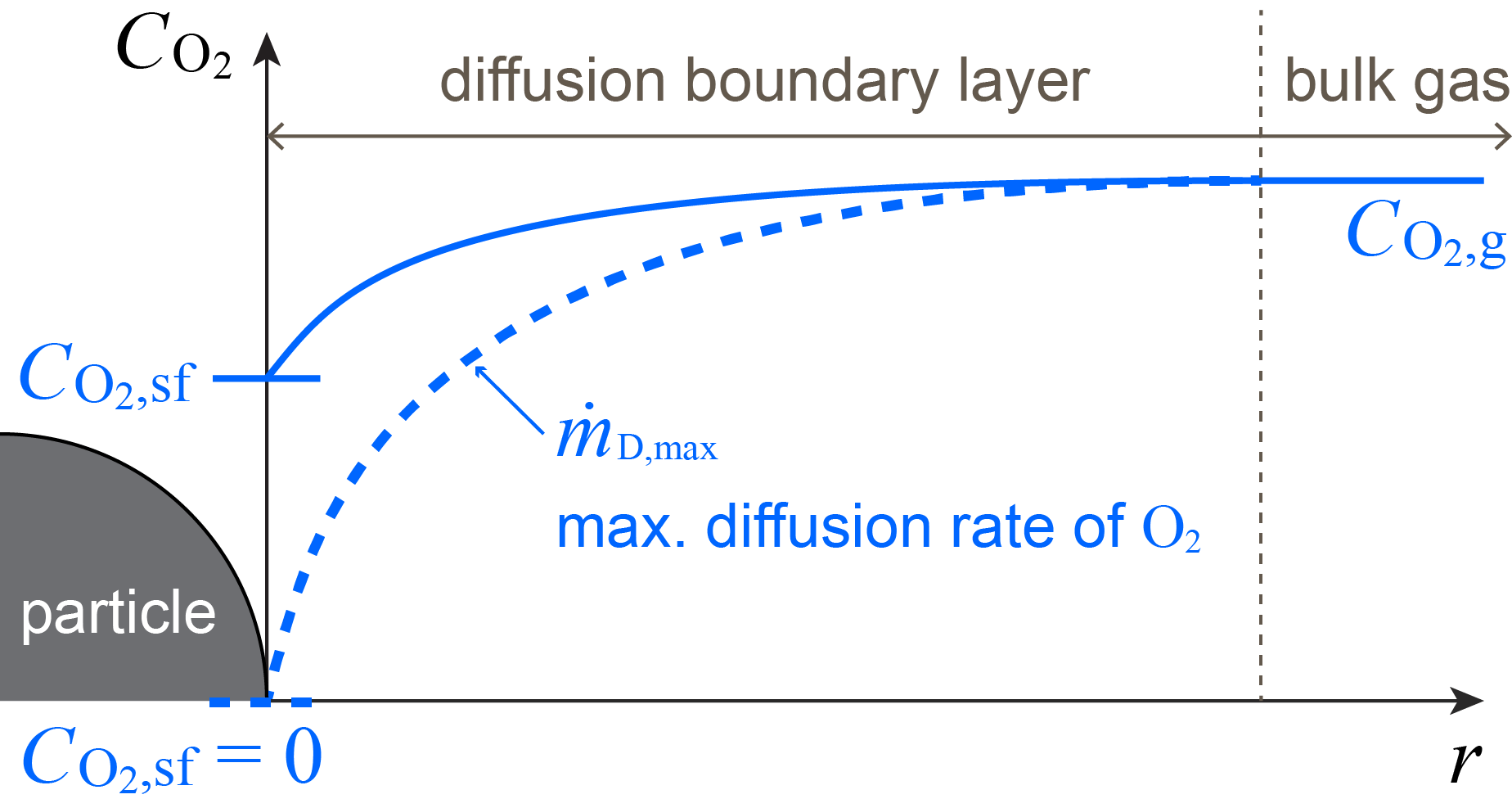
For $C_{{}\mathrm{O}{\vphantom{\mathrm{X}}}_{\smash[t]{\mathrm{2}}}\mathrm{,sf}}>0$, the kinetic rate is less than the maximum rate of $\text{O}{\vphantom{\text{X}}}_{\smash[t]{\text{2}}}$ diffusion, i.e., $\dot{m}_{\mathrm{R}}<\dot{m}_{\mathrm{D,max}}$, and the $\text{O}{\vphantom{\text{X}}}_{\smash[t]{\text{2}}}$ consumption rate of the particle, $\dot{m}_{{}\mathrm{O}{\vphantom{\mathrm{X}}}_{\smash[t]{\mathrm{2}}}}$, is completely controlled by the solid-phase kinetics. When $C_{{}\mathrm{O}{\vphantom{\mathrm{X}}}_{\smash[t]{\mathrm{2}}}\mathrm{,sf}}=0$, the maximum $\text{O}{\vphantom{\text{X}}}_{\smash[t]{\text{2}}}$ diffusion rate is reached such that $\dot{m}_{{}\mathrm{O}{\vphantom{\mathrm{X}}}_{\smash[t]{\mathrm{2}}}}$ must be equal to $\dot{m}_{\mathrm{D,max}}$. Considering the nature of solid-phase iron oxidation, the generic $k$-$\beta$ model can thus be specialized to a switch-type model between the kinetic- and external-diffusion-controlled oxidation rates as:

$$\begin{cases}\dot{m}_{{}\mathrm{O}{\vphantom{\mathrm{X}}}_{\smash[t]{\mathrm{2}}}}=\dot{m}_{\mathrm{R}}&\mathrm{if}\;\dot{m}_{\mathrm{R}}<\dot{m}_{\mathrm{D,max}}\\ \dot{m}_{{}\mathrm{O}{\vphantom{\mathrm{X}}}_{\smash[t]{\mathrm{2}}}}=\dot{m}_{\mathrm{D,max}}&\mathrm{otherwise}\end{cases}\;,$$

(28)

to more accurately describe the transitions between the particle combustion regimes at temperatures greater than $T_{\mathrm{ign}}$. Once a particle transitions into external-diffusion-limited combustion, the total reaction rate of $\text{O}{\vphantom{\text{X}}}_{\smash[t]{\text{2}}}$, $\dot{m}_{{}\mathrm{O}{\vphantom{\mathrm{X}}}_{\smash[t]{\mathrm{2}}}}$, is partitioned into the formation rates of FeO and $\text{Fe}{\vphantom{\text{X}}}_{\smash[t]{\text{3}}}\text{O}{\vphantom{\text{X}}}_{\smash[t]{\text{4}}}$ based on the ratio between the kinetic rates (as shown in Fig. 2) of FeO and $\text{Fe}{\vphantom{\text{X}}}_{\smash[t]{\text{3}}}\text{O}{\vphantom{\text{X}}}_{\smash[t]{\text{4}}}$ formation at the corresponding $T_{\mathrm{p}}$, $X_{{}\mathrm{FeO}}$, and $X_{{}{}\mathrm{Fe}{\vphantom{\mathrm{X}}}_{\smash[t]{\mathrm{3}}}\mathrm{O}{\vphantom{\mathrm{X}}}_{\smash[t]{\mathrm{4}}}}$. Figure 13 shows the comparison between $\dot{m}_{\mathrm{R}}$ (dash-dotted curve) and $\dot{m}_{\mathrm{D,max}}$ (solid curve) resulting from the unsteady model for an isolated particle of $d_{\mathrm{p,0}}=$20\text{\,}\mathrm{\SIUnitSymbolMicro m}$$ in air. When $\dot{m}_{\mathrm{R}}$ exceeds $\dot{m}_{\mathrm{D,max}}$, it indicates the transition of a particle from a kinetic-controlled to an external-diffusion-controlled combustion. The results of $\dot{m}_{\mathrm{R}}$ and $\dot{m}_{\mathrm{D,max}}$ stop when $T_{\mathrm{p}}$ reaches the melting point (m.p.) of FeO.