Brane-world asymptotics in a nonlinear fluid bulk
Abstract
We present recent results on the asymptotics of a brane-world that consists of a flat 3-brane embedded in a five-dimensional bulk. The bulk matter is modelled by a fluid that satisfies a nonlinear equation of state of the form , where p is the ‘pressure’ and is the ‘density’ of the fluid. We show that for appropriate ranges of the parameters and , it is possible to construct a regular solution, compatible with energy conditions, that successfully localizes gravity on the brane. These results improve significantly previous findings of the study of a bulk fluid with a linear equation of state.
keywords
brane-worlds, singularities1 Introduction
In this paper, we review very recent work, presented in [1], on the asymptotic behaviors of a class of brane-worlds. The models consist of a flat 3-brane embedded in a five-dimensional bulk filled with a fluid that satisfies a nonlinear equation of state , where p is the ‘pressure’ and is the ‘density’ of the fluid and , are constants.
Such an equation of state, has been studied in cosmology for its contribution in avoiding big-rip singularities during late time asymptotics [2, 3, 4], in obtaining inflationary models with special properties [5], in unifying models of dark energy and dark matter [6, 7], as well as in studies of singularities [8, 9, 10].
Our goal in studying these brane-world models, is to find a solution that is regular and meets physical requirements set by energy conditions and localization of gravity on the brane. In our previous work in [11, 12, 13, 14, 15, 16], which extended work done in brane-worlds with scalar fields [17, 18, 19], we studied a -brane (flat or curved) and a fluid with a linear equation of state . We found that such a solution becomes possible only for the special value of and only for a flat brane. These results gave us the motivation to explore whether the generalization of the linear equation of state to a nonlinear one, could have a decisive impact in finding a solution with all required properties and valid for a wide range of and . This exploration turned out to be very fruitful, and we were able to find in [1] such solutions for a flat brane and a fluid with and .
As the analysis of the nonlinear equation of state is quite complicated, for the most part of this paper, we will focus on the study of a specific value of , which is simpler for illustration and offers important insight on the behavior of solutions for general .
The structure of this paper is the following: In Section 2, we set up our model and derive the field equations. In Section 3, we formulate the null energy condition which we embody in our solutions later in Section 4. In Section 5, we derive a matching solution for the specific value of and based on this solution, we calculate, in Section 6, the four-dimensional Planck mass. Finally, in Section 7, we discuss briefly the asymptotic behaviors of solutions for general .
2 Setup of brane-world
To set up our model, we start by considering a flat 3-brane embedded in a five-dimensional bulk with a metric of the form,
| (1) |
where is the warp factor and is the four-dimensional flat metric, i.e.,
| (2) |
The timelike coordinate is denoted by and the spacelike ones by . In our notation, Capital Latin indices are taken as while lowercase Greek indices range as . The 5-dimensional Riemann tensor is defined by the formula,
| (3) |
the Ricci tensor is the contraction,
| (4) |
and the five-dimensional Einstein equations on the bulk space are given by,
| (5) |
Next, we set up the bulk matter component by considering a bulk fluid with an energy-momentum tensor of the form,
| (6) |
where is the ‘pressure’ and is the ‘density’ which we take as functions only of the extra dimension . In (6), the velocity vector field is , that is , parallel to the -dimension. We assume that the pressure and density are interconnected by the following nonlinear equation of state
| (7) |
with and constants.
The Einstein equations can be written as
| (8) | |||||
| (9) |
with the prime denoting differentiation with respect to . The equation of energy-momentum conservation, on the other hand,
becomes
| (10) |
At this point, it is useful to clarify the terminology that we use in what follows. We use the term finite-distance singularities to refer to the following singular behaviors of , occurring within a finite distance :
- •
, as (collapse singularity),
- •
, as (big-rip singularity).
With , we denote a finite value of designating the position of the singularity. The above behaviors may be accompanied, in general, by a divergence in the density, or, even in the pressure of the fluid. Note that, these singularities are not related to geodesic incompleteness as in standard cosmology, but rather on a pathological behavior of the warp factor. In the absence of finite-distance singularities, we call the solutions regular and include in this category the behaviors of the warp factor given above, provided that these occur only at infinite distance, i.e .
We are interested to see, if it is possible to find solutions of Eqs. (8)-(10) that rectify previous findings of solutions of brane-worlds with linear bulk fluids studied in [11, 12, 13, 14, 15, 16]. As mentioned in the introduction, excepting the case of a flat brane and a fluid with , the main problem that we faced in the study of a linear bulk fluid, is that regular solutions that exist in the case of curved branes, or even singular ones out of which we can construct a regular matching solution for both flat and curved branes, lead to a challenging compromise: they either satisfy energy conditions, or, localize gravity on the brane. Therefore, a solution arising from the consideration of this different and more complicated type of fluid would be preferable and worth examining in detail, if it has each one of the following characteristics:
- •
it is regular (no finite-distance singularities)
- •
it satisfies physical conditions, such as energy conditions
- •
it leads to a finite four-dimensional Planck mass, thus, it localizes gravity on the brane.
We can simplify the situation of finding such a solution, by incorporating, for example, the energy conditions a priori. As we show in the next Sections this is indeed possible. The regular nature as well as the requirement of a finite four-dimensional Planck mass can be checked as a subsequent step, since to accomplish that, we first need to find the exact form of the warp factor and density.
3 The null energy condition
We are going to derive the null energy condition for our type of nonlinear bulk fluid described by (6) and (7) and transform it to a condition imposed on the density and parameters and of the equation of state.
To achieve this, we follow the technique analysed in [14, 16]. We start by recalling that the metric (1) and the bulk fluid (6) and (7) depend only on the extra dimension and they are therefore static with respect to the time coordinate . Such fluid can be viewed as an anisotropic one with energy-momentum tensor
| (11) |
where , and . As a next step, we compare (6) with (11) and find that the following relations should hold
| (12) | |||||
| (13) | |||||
| (14) |
We note that once we combine the last two relations we get
| (15) |
which means that this type of matter satisfies a cosmological constant-like equation of state. Substituting (12)-(15) in (11), we find that
| (16) |
Here, we focus only on the null energy condition according to which, every future-directed null vector should satisfy [20]
| (17) |
This means that we should have
| (18) |
from which we find
| (19) |
after inputting the equation of state . Now, Eq. (19) can be written as
| (20) |
and since from Eq. (8), we arrive at the the final form of the null energy condition, which reads
| (21) |
In the next Section, we are going to incorporate this condition in the process of deriving our solutions.
4 Regular solution
We start solving the system of Eqs. (8)-(10), by first integrating the continuity equation (10) to find the relation between the warp factor and the density. In the integration process we arrive at a logarithmic term of the form . To incorporate from the beginning the null energy condition (21), we choose to ignore the absolute value and simply put this term equal to . The resulting relation between and is
| (22) |
where
| (23) |
with being the initial conditions. According to (21) this translates to .
It is crucial to note that there is a singularity in the density () for and
| (24) |
However, it is possible to avoid this singularity, by restricting the range of the parameter , only to negative values, which we do in the analysis that follows.
Substituting Eq. (22) in Eq. (8) and integrating, we obtain,
| (25) |
The complicated integral on the LHS of Eq. (25), can be greatly simplified for those values of that make a negative integer. This is possible when , with and a positive integer.
Clearly, the simplest case is for which corresponds to . Then and we can directly integrate Eq. (25) to get the solution in the following implicit form
| (26) |
where is an integration constant. It is straightforward to see that this solution is regular: all possible singular behaviors of , namely and happen only for infinite values of with and either vanishing there, or, approaching finite nonzero values. In particular, we have
| (27) | |||||
| (28) |
Summarizing, the solution for has already two out of the three good qualities mentioned in the previous Section: it is regular and at the same time satisfies the null energy condition. In the following section, we construct an appropriate matching solution out of this solution, which leads to a finite four-dimensional Planck mass, thus fitting perfectly the profile of a plausible solution.
As for the asymptotics for general values of , it is interesting to note here that even though the case of is the simplest possible one for the nonlinear fluid, further analysis performed in [1], shows that this case is significant in the sense that it can act as a guide for the whole range of values of . This follows from the fact that all of its good physical properties are, in a way, inherited to all cases with .
5 Matching solution for
For , a matching solution that leads to a finite four-dimensional Planck mass, can be constructed in the following way: First, we write down the two different branches of solution of Eq. (26),
| (29) | |||||
| (30) |
using the notation to describe the solutions for the choice of sign in Eq. (26). Similarly, the notation , describes the values of and , respectively, on the branch of .
Second, in order to gain a complete idea of the behavior of , we study the shape of the curve of by calculating the first and second derivative of . These read
| (31) | |||||
| (32) |
For our choice of integration constants and parameters, and , Eq. (31) shows that is strictly increasing for all values of . Also, Eq. (32) shows that the graph of changes from concave downward on to concave upward on , making the point , an inflection point of the graph of .
On the other hand, the first two derivatives of are exactly the opposites of the ones of given in Eq. (31) and Eq. (32) above. This means that is strictly decreasing and the graph of changes from concave upward on to concave downward on , with being an inflection point of the graph of .
We can match the two branches at their common inflection point by making an appropriate choice of the constants and . This is a third step in the matching process. Naturally, we assume that the warp factor is continuous
| (33) |
and that, of course, the inflection point has the same coordinate through the two branches, which leads to
| (34) |
and yields the following relation between and ,
| (35) |
or,
| (36) |
There is an axis of symmetry at , with given by
| (37) |
Since the embedding of the brane introduces a symmetry in the bulk, it is natural to position the brane at . Without loss of generality and in order to simplify our expressions, we can place the brane at , that is we take in . This will set the values of to
| (38) |
The matching solution described by Eq. (29) and (30) that satisfies the above boundary condition can be written as
| (39) |
It is essential that the density is well defined and continuous at the position of the brane . Here, we find
| (40) |
where denotes and it is an abbreviation of .
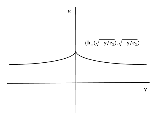
The graph of is depicted in Fig. 1 with a thick solid and dashed line, while the graph of , in the same Figure, is depicted with a thin solid and dashed line. The matching solution is build up only from the solid parts of both graphs, as this is the only choice that leads to a solution with a finite four-dimensional Planck mass. In Fig. 2, we have rotated the axes of Fig. 1, for a more convenient view of the evolution of the warp factor as a function of .

Finally, we take into account the jump of the derivative of the warp factor across the brane and find, for our type of geometry, the following junction condition
| (41) |
where is the tension of the brane. Using Eq. (39) in the above equation we can deduce the form of the brane tension, this reads
| (42) |
where the last equality is derived by using Eq. (40).
This completes the construction of a viable matching solution for . In the next Section, we are going to show that this solution also leads to a finite four-dimensional Planck mass.
6 Localization of gravity for
To calculate the value of the four-dimensional Planck mass, , we use the following integral (see [14, 16, 1, 21]),
| (43) |
We can deduce the behaviour of as from Eq. (39). We find
| (44) |
where the symbol is used to signify ‘behaves according to’, and using the symmetry of Eq. (39), we can write the above integral in the following form
| (45) |
Taking and keeping in mind that , it follows that the four-dimensional Planck mass remains finite and is proportional to
In conclusion, we have seen a specific example of the nonlinear equation of state , for which it is possible to construct a regular matching solution compatible with the null condition and which also localizes gravity on the brane. In the discussion below, we outline what happens for extended ranges of values of .
7 Discussion
We briefly review in this Section, the behavior of solutions for general , a detailed analysis can be found in [1].
The key factor that determines whether a solution of Eqs. (8)-(10), is regular, or, singular, is the ordering of with respect to the value one: for , we encounter singular solutions, whereas, for the solutions are regular.
Before presenting the solutions for general , we emphasize that for , where is a positive integer, the integral on the LHS of Eq. (25) cannot in general be calculated directly. However, we can still deduce the behaviors of solutions by expressing them in terms of the Gaussian hypergeometric function .
In particular, for , the solution is given implicitly in terms of a hypergeometric function and reads
| (46) |
As shown in [1], this solution has a finite-distance singularity at , with
| (47) | |||
| (48) |
The behaviors of and above, have been deduced from Eq. (7) and Eq. (22).
For , on the other hand, we have the following types of solution. First, we have the general form of solution for , with a positive integer, which is
| (49) |
Second, for we have the following solution
| (50) | |||||
Finally, the case of is more complicated: we have forms of solutions valid for , with a positive integer such that , and given by
| (51) | |||||
All solutions for are free from finite-distance singularities, and their asymptotic behaviors are
| (52) | |||||
| (53) |
The procedure for deriving a matching solution with a finite four-dimensional Planck mass, presented in the previous Sections, can still be performed for all solutions with and can be found in [1].
Summarizing, the effect of the nonlinear equation of state is catalytic in the process of creating a regular solution with essential physical properties and valid for a wide range of parameters. It is left to be seen from a physics point of view, what are the possible field realizations that could lead to such an equation of state.
Acknowledgments
Work partially performed by I.A. as International professor of the Francqui Foundation, Belgium.
References
- [1] I. Antoniadis, S. Cotsakis, I. Klaoudatou, Regular branewords with nonlinear bulk-fluids, Eur. Phys. J. C 81, (2021). [arXiv:2106.15669v2 [hep-th]].
- [2] S. K. Srivastava, Future Universe With Without Big Smash, Phys. Lett. B 619, 1-4 (2005). [arXiv:0407048v4 [astro-ph]].
- [3] P. F. Gonzalez-Diaz, You need not be afraid of phantom energy, Phys. Rev. D 68, 021303 (2003). [arXiv:0305559 [astro-ph]].
- [4] A. V. Astashenok, S. Nojiri, S. D. Odintsov, A. V. Yurov. Phantom Cosmology without Big Rip Singularity, Phys. Lett. B 709, 396-403 (2012). [arXiv:1201.4056 [gr-qc]].
- [5] J. D. Barrow, Graduated inflationary universes, Phys. Lett. B 235, 40-43 (1990).
- [6] A. Y. Kamenshchik, U. Moschella, V. Pasquier, An alternative to quintessence, Phys. Lett. B 511, 265-268 (2001). [arXiv:0103004 [gr-qc]].
- [7] M. C. Bento, O. Bertolami, A. A. Sen., Generalized Chaplygin gas, accelerated expansion and dark energy-matter unification, Phys. Rev. D 66, 043507 (2002). [arXiv:0202064 [gr-qc]].
- [8] S. Cotsakis, I. Klaoudatou, Future Singularities of Isotropic Cosmologies, J. Geom. Phys. 55, 306-315 (2005). [arXiv:0409022 [gr-qc]].
- [9] S. Cotsakis, I. Klaoudatou, Cosmological Singularities and Bel-Robinson Energy, J. Geom. Phys. 57, 1303-1312 (2007). [arXiv:0604029 [gr-qc]].
- [10] S. Nojiri, S. D. Odintsov, S. Tsujikawa, Properties of singularities in (phantom) dark energy universe, Phys. Rev. D 71, 063004 (2005). [arXiv:0501025 [hep-th]].
- [11] I. Antoniadis, S. Cotsakis, I. Klaoudatou, Braneworld cosmological singularities, Proceedings of the 11th Marcel Grossmann Meeting on General Relativity 3, 2054-2056 (2007). [arXiv:0701033 [gr-qc]].
- [12] I. Antoniadis, S. Cotsakis, I. Klaoudatou, Brane singularities and their avoidance, Class. Quant. Grav. 27, 235018 (2010). [arXiv:1010.6175 [gr-qc]].
- [13] I. Antoniadis, S. Cotsakis, I. Klaoudatou, Brane singularities with mixtures in the bulk, Fortschr. Phys. 61, 20-49 (2013). [arXiv:1206.0090 [hep-th]].
- [14] I. Antoniadis, S. Cotsakis, I. Klaoudatou, Enveloping branes and braneworld singularities, Eur. Phys. J. C 74, 3192 (2014). [arXiv:1406.0611v2 [hep-th]].
- [15] I. Antoniadis, S. Cotsakis, I. Klaoudatou, Dynamics and asymptotics of brane-worlds, Proceedings of the 13th Marcel Grossmann Meeting on General Relativity 3, 1859-1861 (2015).
- [16] I. Antoniadis, S. Cotsakis, I. Klaoudatou, Curved branes with regular support, Eur. Phys. J. C 76, 511 (2016). [arXiv:1606.09453 [hep-th]].
- [17] N. Arkani-Hamed, S. Dimopoulos, N. Kaloper, R. Sundrum, A small cosmological constant from a large extra dimension, Phys. Lett. B 480, 193-199 (2000). [arXiv:0001197v2 [hep-th]].
- [18] S. Kachru, M. Schulz, E. Silverstein. Bounds on curved domain walls in 5d gravity, Phys. Rev. D 62, 085003 (2000). [arXiv:0002121 [hep-th]].
- [19] S. S. Gubser, Curvature singularities: The good, the bad, and the naked, Adv. Theor. Math. Phys. 4, 679-745 (2000). [arXiv:0002160 [hep-th]].
- [20] E. Poisson, A Relativist’s Toolkit (Cambridge University Press, 2004).
- [21] S. Forste, H. P. Nilles and I. Zavala, Nontrivial Cosmological Constant in Brane Worlds with Unorthodox Lagrangians, JCAP 07, 007 (2011). [arXiv:1104.2570 [hep-th]].