Measurement-based time evolution for quantum simulation of fermionic systems

Unbiased quantum simulation Feynman 1982; Georgescu et al. 2014 of intractable models aids in validating approximations. Compelling open problems include the two-dimensional Hubbard model of the cuprates and, more generally, materials and quantum chemistry models Abrams and Lloyd 1997; Abrams and Lloyd 1999; Ortiz et al. 2001; Somma et al. 2002; Aspuru-Guzik 2005; Kassal et al. 2011; Yung et al. 2014; Wecker et al. 2014; McClean et al. 2014; Wecker et al. 2015; Bauer et al. 2016; McClean et al. 2017; Babbush et al. 2018; Poulin et al. 2018; McArdle et al. 2020. Such interacting fermionic models are typically NP-hard because they suffer from the fermion sign problem Troyer and Wiese 2005 and are generally parameterized as: $H=\sum_{i,j}w_{ij}c_{i}^{\dagger}c_{j}^{\vphantom{\dagger}}+\sum_{i,j,k,l}V_{ijkl}c_{i}^{\dagger}c_{j}^{\dagger}c_{k}^{\vphantom{\dagger}}c_{l}^{\vphantom{\dagger}}$, where $c_{j}^{\dagger}$ creates a fermion in quantum state $j$ (a composite index for spin, lattice site, etc.) and $w_{ij}(V_{ijkl})$ is the single (two)-particle Hamiltonian matrix element. Since they are NP-hard, classical simulation time increases exponentially with particle number. Unbiased quantum simulation of models captured by $H$ will therefore offer high impact benchmarks. Variational quantum algorithms offer promise on near-term devices Moll et al. 2018 because they can be used to rigorously bound ground state energies.

Recent work Ferguson et al. 2021 combines a variational quantum algorithm with measurement-based quantum computing (MBQC) Raussendorf and Briegel 2001; Raussendorf et al. 2003 for efficient management of variational ansatz states. MBQC starts with a resource state, e.g., a graph state such as the square lattice cluster state (SLCS), formed by taking qubits aligned along the Pauli-$x$ direction and then entangling them pairwise with controlled-$Z$ gates. All quantum algorithms can then be executed using just single-qubit measurements on the resource state. MBQC-based variational algorithms Ferguson et al. 2021 can therefore use measurements to bound ground state energies.

Phase-estimation-based quantum simulation algorithms Kitaev 1995; Lloyd 1996; Abrams and Lloyd 1999; Berry and Wiseman 2000; Higgins et al. 2007; Svore et al. 2014 can go beyond variational bounds to yield exact eigenfunctions and eigenvalues of $H$ for use in benchmarking excited state properties. In circuit-based quantum computing (CBQC), such algorithms take an input wave function $|\psi_{\text{I}}\rangle$ and repeatedly apply quantum gates to time-evolve $H$ with $M$ small time steps $\delta t_{g}$ to eventually extract information. Quantum algorithms based on this procedure yield an advantage over classical algorithms but for runtimes that increase exponentially with the required bit precision in, e.g., eigenvalues. Long runtimes can be prohibitive Peruzzo et al. 2014; McClean et al. 2014; Wecker et al. 2015 if, for $N_{g}$ gates per time step, the qubits cannot be kept coherent for long execution times, $T_{\rm C}\sim MN_{g}\delta t_{g}$.

We propose revisiting phase-estimation-based quantum simulation runtime from the MBQC perspective. We consider the following regime: (i) A large number of qubits are available, (ii) the time taken for an accurate single-qubit measurement $\delta t_{m}$ can be made small enough to avoid decoherence of the resource state, and (iii) the entangling gates are performed in parallel mostly at the beginning. Assumption (iii) allows slow/error-prone entangling gates to be implemented and error corrected in a time that is negligible compared with the time to execute all measurements.

In this letter, we explicitly map real-time evolution in CBQC (repeated application of gates that take a finite amount of time) to repeated measurement in MBQC Raussendorf et al. 2003. To this end, we make the following advances: (i) We construct a route to use MBQC to effectively time-evolve $H$ using just single-qubit measurements. We show that long effective time evolution corresponds to $M$ sequential measurement rounds in MBQC, thus requiring coherence among non-measured qubits for a total time, $T_{\rm M}\sim MN_{m}\delta t_{m}$, where $N_{m}$ is the number of measurements per round. (ii) We construct an example hybrid MBQC algorithm with a quantum phase-estimation-based subroutine that yields exact eigenenergies: quantum eigenvalue estimation using an offline (classical) time series Somma et al. 2002; Somma 2019; see Fig. 1(a). (iii) We apply the algorithm to solve the Kitaev Kitaev 2001; Kitaev and Laumann 2008 and Hubbard Essler et al. 2005 chains because they can be solved exactly and can therefore be accurately checked as first implementations. To compare $T_{\rm M}$ and $T_{\rm C}$ for our algorithm, we compute scaling of MBQC measurement time and precision costs as well as gate counts in an equivalent CBQC algorithm.

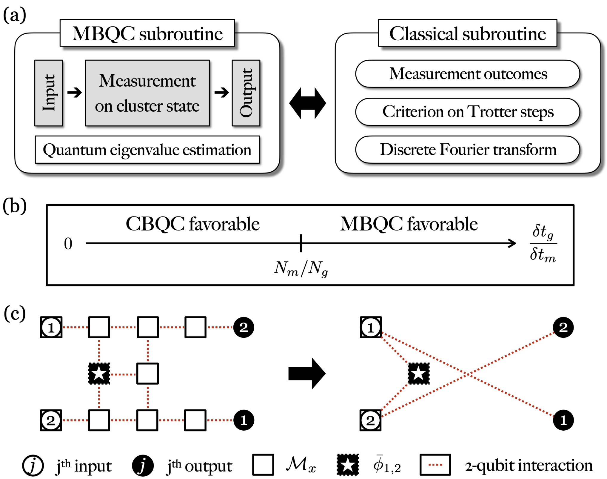
Our central finding is that MBQC can yield a runtime advantage over CBQC, i.e., $T_{\rm M}<T_{\rm C}$, by shifting the burden of requiring low $\delta t_{g}$ but high-fidelity gates in CBQC simulation to the requirement of low $\delta t_{m}$ and high single-qubit measurement precision in MBQC simulation. Figure 1(b) summarizes our finding by showing that, if $\delta t_{g}/\delta t_{m}$ is large, MBQC will have shorter runtimes. Here, $N_{m}/N_{g}$ is set by the algorithm. We find that graph state compactification Hein et al. 2004 can yield hybrid MBQC algorithms with $N_{m}/N_{g}=1$. In this letter, therefore, we establishe a route to use improvements in quantum sensing Degen et al. 2017 to advance the state of the art in quantum simulation with effective time evolution.

Time evolution of Hamiltonians containing noncommuting terms $H_{1}$ and $H_{2}$ requires a decomposition. The first-order Trotter-Suzuki decomposition is simplest Trotter 1959; Suzuki 1993: $\exp[-i(H_{1}+H_{2})t]=[\exp(-iH_{1}t/M)\exp(-iH_{2}t/M)]^{M}+\mathcal{O}[(t/M)^{2}]$. Here the time step $t/M$ is repeated $M$ times until the output state is converged within a tolerance $\delta_{\rm T}$ Com a, and $\hbar=1$.

To map between fermions and qubits in $H$, we use the Jordan-Wigner (JW) transformation Jordan and Wigner 1928: $c_{j}^{\dagger}=\prod_{k=1}^{j-1}[-\sigma_{z}^{(k)}]$ $[\sigma_{x}^{(j)}+i\sigma_{y}^{(j)}]/2$, where $\sigma_{a}$ with $a\in\{x,y,z\}$ are the Pauli matrices. Long JW strings containing $N$ qubits can arise in certain models, e.g., those with long-range hopping/interaction in $H$. Longer-range terms allow simulation of higher-dimensional fermionic models $H$ because they map to one-dimensional chains with long-range hopping and long-range interaction. Time evolution of a string requires the ability to execute nontrivial unitaries: $R_{a_{1}a_{2}\cdots a_{N}}^{(1,2\cdots N)}(\theta)=\exp[-i(\theta/2)\prod_{j=1}^{N}\sigma_{a_{j}}^{(j)}]$, where $\theta$ is a rotation angle.

The JW transformation enables construction of a time-to-angle mapping for MBQC simulation. Figure 1(c) shows an example measurement pattern needed for time evolution of a hop between neighboring sites, $c_{1}^{\dagger}c_{2}^{\vphantom{{\dagger}}}$ $+c_{2}^{\dagger}c_{1}^{\vphantom{{\dagger}}}$. In the absence of the central measurement (star), the measurement pattern swaps information on qubits 1 and 2 Raussendorf et al. 2003; SM. However, the additional adaptive measurement in the second round of measurements with $\bar{\phi}_{1,2}$ on the central qubit (star) incorporates results from the first round to yield Raussendorf et al. 2003 $R_{zz}^{(1,2)}(\theta)|\psi_{\text{I}}\rangle$, where $\theta$ defines the part not relying on random measurement outcomes in $\bar{\phi}_{1,2}$. This operation is a time propagator, and one can show, see Supplemental Material SM, that, with a few more measurements, this measurement pattern effectively time-evolves a hop between sites 1 and 2.

Figure 1(c) generalizes to time evolution of longer-range terms in $H$ on a larger SLCS using only $\mathcal{O}(1)$ adaptive measurements. Consider, e.g., a long-range hop between sites $1$ and $N$: $c_{1}^{\dagger}c_{N}^{\vphantom{{\dagger}}}+c_{N}^{\dagger}c_{1}^{\vphantom{{\dagger}}}$. To implement effective time evolution of the JW term, we must execute the unitary $R_{zz\cdots z}^{(1,2\cdots N)}(\theta)$ (and follow up with a few rotations on the end qubits). This can be implemented with two rounds of measurements on $[(2N-1)^{2}$ $-(N-1)]$ qubits on the central area of the measurement pattern (excluding input and output qubits). The first round measures all but a central qubit, and the second round measures just the central qubit in an adaptive basis, see Supplemental Material SM, thus showing a considerable simplification in implementing long JW strings.

The number of measurements and qubits needed for effective time evolution on a SLCS, e.g., the left side of Fig. 1(c), can be significantly reduced. The Gottesman-Knill theorem Gottesman 1999 shows that all qubits with Pauli-$x$ measurements can be excluded since Clifford operations can be efficiently executed classically. After mathematically removing local Pauli measurements, the SLCS maps to a compactified cluster state (CCS) Hein et al. 2004. The mappings show that a much smaller graph state is needed. For example, the right side of Fig. 1(c) shows an equivalent execution of $R_{zz}^{(1,2)}(\theta)$ (see Supplemental Material SM for a proof), where the number of qubits (measurements) reduces from 12(10) to 5(3). In general, a CCS offers a reduction in measurement and qubit overhead for executing effective time evolution using $R_{zz\cdots z}^{(1,2\cdots N)}(\theta)$ by as much as $\mathcal{O}(N^{2})$, depending on which CCS is chosen. We construct example time-evolution subroutines on SLCSs with the understanding that use of a CCS reduces the number of required qubits and measurements at the expense of modifying qubit connectivities which is efficiently programmable Anders and Briegel 2006.

We construct an MBQC subroutine for time evolution of an example model with noncommuting terms, the Kitaev chain Kitaev 2001; Kitaev and Laumann 2008:

where $w\geq 0$ is the hopping and pairing energy, $\mu\geq 0$ is the chemical potential, and $\delta n_{j}=c_{j}^{\dagger}c_{j}^{\vphantom{\dagger}}-1/2$. The ground state exhibits a quantum phase transition at $\mu=2w$ between a non-topological strong-coupling phase ($\mu>2w$) and a topological weak-coupling phase ($\mu<2w$).

We map fermions to qubits to construct both circuit- and measurement-based time propagators. The JW transformation maps $H_{\text{K}}$ to the quantum Ising model. The first-order Trotterized form of $\exp(-iH_{\text{K}}t)$ is

where $g_{\mu}=\mu/(2w)$ and

is a measurement angle. Equation (2) can be implemented in two different ways: using real-time evolution in CBQC or effective time evolution in MBQC, where $M$ dictates the circuit or measurement depth, respectively. Equation (3) is central because it maps real time $t$ to measurement angle.

We use the stabilizer formalism to map Eq. (2) to effective time evolution in MBQC. Figure 2(a) shows the measurement pattern implementing Eq. (2) to time-evolve input qubits 1-4 (open circles) with just single-qubit measurements. The measurement angles in the $x$-$y$ plane are

where $\psi^{r}\in\{\pm\alpha,\pm\beta,\gamma\}$ for $r=\pm 1,\pm 2,3$, $-\alpha=\beta=\gamma=$ $\pi/2$, and $P_{\theta}=(-1)^{S_{\theta}^{\text{K}}}$. Here, $S_{\theta}^{\text{K}}$ accumulates all measurement outcomes during single-qubit measurements and is derived in the Supplemental Material SM. The measurement outcomes are also used for offline processing with a byproduct operator, see Supplemental Material SM, that defines the basis for interpreting output measurements.

The left, middle, and right panels depict measurements [stars in Fig. 2(a)] that entangle input qubits 1-2, 2-3, and 3-4, respectively. The measurement pattern in Fig. 2(a) and Eq. (4) define the full effective time-evolution algorithm for a Kitaev chain of any $N$ or $M$ because additional panels in Fig. 2(a) can be concatenated, see Supplemental Material SM. The red dots and arrows show information flow for use in concatenation.

We now turn to the Hubbard chain Essler et al. 2005 with a longer JW string and an important interaction term:

where $\sigma\in\{\uparrow,\downarrow\}$, $U$ is the Hubbard interaction strength, and $n_{j,\sigma}=c_{j,\sigma}^{\dagger}c_{j,\sigma}^{\vphantom{\dagger}}$. To map fermions to qubits, we introduce Camp 1974 spinless fermion operators: $\tilde{c}_{2j-1}=c_{j,\uparrow}$ and $\tilde{c}_{2j}=c_{j,\downarrow}$. The JW mapping then leads to an equivalent qubit Hamiltonian: $(w/2)\sum_{j=1}^{2N-2}(\sigma_{x}^{(j)}$ $\sigma_{z}^{(j+1)}\sigma_{x}^{(j+2)}+\sigma_{y}^{(j)}\sigma_{z}^{(j+1)}\sigma_{y}^{(j+2)})$ $+(U/4)\sum_{j=1}^{N}(\mathbb{I}_{2j-1}+\sigma_{z}^{(2j-1)})(\mathbb{I}_{2j}+\sigma_{z}^{(2j)})$, where the JW strings used for the hopping terms need a three-qubit entangling gate, and $\mathbb{I}={\rm diag}(1,1)$. The first-order Trotterized form of $\exp(-iH_{\text{H}}t)$ is

where $g_{U}=U/(2w)$.

Equation (6) can be used in CBQC or mapped to single-qubit measurements in MBQC. Figure 2(b) depicts the $N=2$ measurement pattern for Eq. (6) with measurement angles:

where $\psi^{r}\in\{\pm\alpha,\pm\beta,$ $\pm\gamma,\pm\lambda\}$ for $r=\pm 1,\pm 2,\pm 3,\pm 4$, $\lambda=\alpha$, and $P_{\theta}=(-1)^{S_{\theta}^{\text{H}}}$. $S_{\theta}^{\text{H}}$ is derived in Ref. SM. The Hubbard chain measurement pattern can also be concatenated to time-evolve larger $N$ or $M$ SM, and overhead can be significantly reduced in a CCS.

Both examples, Eqs. (4) for $H_{\text{K}}$ and Eqs. (7) for $H_{\text{H}}$, demonstrate constraints on effective time evolution. Long effective time evolution from a larger number of Trotter steps in MBQC corresponds to smaller measurement angles since $\phi_{M}\propto 1/M$. Repeated small-angle measurements (long effective time evolution) in MBQC therefore require improvements in qubit measurement precision as opposed to faster gates in CBQC.

To demonstrate resource requirements, we construct a minimal hybrid quantum eigenvalue estimation algorithm by combining MBQC subroutines with an offline time-series estimator [Fig. 1(a)]. A $|\psi_{\text{I}}\rangle$ close to a desired eigenstate is fed into the MBQC time-evolving subroutine yielding $\langle\psi_{\text{I}}|e^{-iHt}|\psi_{\text{I}}\rangle$ if the output qubits are measured using quantum state tomography (or an ancilla qubit Somma et al. 2002) to find the wavefunction phase relative to the input qubit basis. The MBQC output is obtained $L$ times and used in a classical discrete Fourier transform:

where we define $t_{n}=n\delta t$, $\omega_{m}=m\delta\omega$ ($n,m=0,1,\cdots,L-1$) in units of $\delta t$ and $\delta\omega$ satisfying $\delta\omega\delta t=2\pi/L$. Peaks in $\mathcal{A}(\omega)$ yield eigenvalues of $H$ to within $\delta_{\rm T}$. We introduce the broadening parameter $\eta>0$ for visualization of Lorentzian peaks and as a proxy for experimentally limited resolution.

The main panel in Fig. 3 shows a demonstration result from a simulation using $H_{\text{K}}$ in Eq. (8), where several eigenvalues are returned as peaks. One can show, see Supplemental Material SM, that peak centers are intact while peak weights are shifted for certain types of measurement errors. Figure 3 uses large $L$ and $M$ for clarity but in practice, $L$ and $M$ can be lowered. They are minimized by restricting the search to just the ground state energy, while three independent algorithm input parameters $\delta\omega$, $L$, and $M$ must be chosen to meet three tolerances: (i) $\delta\omega$ should be smaller than $\eta$ to resolve peak structure, (ii) A sum rule tolerance $\delta_{\rm F}>\big|1-\delta\omega\sum_{m=0}^{L-1}\mathcal{A}(\omega_{m})\big|$ sets $L$, and (iii) $M$ is set by requiring $\delta_{\rm T}$ to be much smaller than the first spectral gap.

The number of Trotter steps yields the measurement depth and sets $\phi_{M}$. Large $M$ improves Trotter accuracy at the expense of requiring improved measurement precision (small $\phi_{M}$). To estimate the minimum $M$ needed to obtain ground state energies, we consider $H_{\text{K}}$ with $g_{\mu}=0.01-0.4$. We find empirically, see Supplemental Material SM, that, for each $n$ in Eq. (8), the minimum $M$ varies from $1.8\times 10^{3}$ ($g_{\mu}=0.01$) to $7.8\times 10^{4}$ ($g_{\mu}=0.4$) to resolve the ground state energy of $H_{\text{K}}$ to within $1\%$ of the spectral gap ($\delta_{\rm T}=10^{-2}$) for $\eta=0.02w$, $\delta\omega=0.01w$, $L=46$, and $N=4$. We have checked $N\leq 8$ with other $\eta$, $\delta\omega$, and $L$ combinations and obtained similar results for $M$. In general, the $M$ needed will depend on the model, model parameters, tolerances, and scales as $\mathcal{O}((Nt_{n})^{2}\delta_{\rm T}^{-1})$ Childs et al. 2021, thus implying that the required measurement depth and precision to execute effective MBQC time evolution can become demanding Com b.

Given bounds on $M$, we can estimate measurement precision requirements for $H_{\text{K}}$. Here, $\phi_{M}$ depends on $n$. The largest measurement angle (in units of $2\pi$) needed to implement Eq. (8) with Eq. (4) is $\chi_{L-1}$, where $\chi_{n}\equiv nw/(\delta\omega LM)$. We empirically find, see Supplemental Material SM (far from the critical point at $g_{\mu}=1$), $\chi_{n}\lesssim 0.14$, thus allowing the use of Eq. (3). The smallest measurement angle increment needed in Eq. (4) is $g_{\mu}\chi_{n}$. We find $g_{\mu}\chi_{n}\gtrsim 4.8\times 10^{-4}$ for all $g_{\mu}<1$ and $n$. We therefore see that a large $M$ requires small angle measurements as we implement effective time evolution.

The measurement subroutines defined by Eqs. (4) and (7) allow estimates of resource requirements in our hybrid quantum eigenvalue estimation algorithm. Table 1 shows, see Supplemental Material SM, that, for the local models considered here, a CCS will have $N_{m}/N_{g}=1$. However, with nonlocal qubit terms, e.g., for nonlocal hopping in $H$, MBQC with a CCS will have an $\mathcal{O}(N)$ advantage in measurement vs gate counts in CBQC unless nonlocal gates are used to implement the JW strings Hastings et al. 2014. The number of qubits needed is $\mathcal{O}(M)$ larger for MBQC than for CBQC. MBQC qubit overhead can be lowered by re-entangling measured qubits Raussendorf and Briegel 2001.

Our demonstration algorithms show that unbiased quantum simulation using effective time evolution is possible using only single-qubit measurements on graph states. We find that long MBQC effective time evolution for use in quantum simulation requires high measurement precision to be useful in benchmarking approximate classical algorithms. Alternative time-evolution decompositions Berry et al. 2014; Berry and Novo 2016; Poulin et al. 2018; Childs et al. 2019; Low and Chuang 2017 will lower overhead.

MBQC offers advantages in systems with slow/error-prone entangling gates Briegel et al. 2009, e.g., photonics Kok et al. 2007; Pick et al. 2021 and atoms in optical lattices Raussendorf and Briegel 2001. In the latter case, parallelized collisional gates encoded large SLCSs in long-lived atomic hyperfine states Mandel et al. 2003. Recent progress in single-site measurements Wang et al. 2015 and control Wang et al. 2016 allow optical lattice implementation of MBQC effective time-evolution algorithms.

The above algorithms have a low error threshold Aliferis and Leung 2006; Dawson et al. 2006. An improvement with higher thresholds is available Raussendorf et al. 2006; Raussendorf and Harrington 2007. The above algorithms can also be used in conjunction with an adaptive Bayesian algorithm (instead of a time series) in eigenvalue estimation learning certain types of error Wiebe and Granade 2016; O’Brien et al. 2019.

Finally, applications to higher-dimensional fermionic models are highly desired. Nearest neighbor hoppings/interactions in a higher-dimensional fermionic lattice can be mapped to long-range hoppings/interactions in a chain Somma et al. 2002. After mapping, our hybrid MBQC algorithm can be applied to the chain at the expense of increasing the length of JW strings.