Proton deflectometry with in situ x-ray reference for absolute measurement of electromagnetic fields in high-energy-density plasmas
Abstract
We report a technique of proton deflectometry which uses a grid and an in situ reference x-ray grid image for precise measurements of magnetic fields in high-energy density plasmas. A D3He fusion implosion provides a bright point-source of both protons and x-rays, which is split into beamlets by a mesh grid. The protons undergo deflections as they propagate through the plasma region of interest, whereas the x-rays travel along straight lines. The x-ray image therefore provides a zero-deflection reference image. The line-integrated magnetic fields are inferred from the shifts of beamlets between the deflected (proton) and reference (x-ray) images. We developed a system for analysis of this data, including automatic algorithms to find beamlet locations and calculate their deflections from the reference image. The technique is verified in an experiment performed at OMEGA to measure a non-uniform magnetic field in vacuum, then applied to observe the interaction of an expanding plasma plume with the magnetic field.
I Introduction
Magnetic fields are valuable to control and improve energy confinement in high-energy-density (HED) plasma experiments. Strong, 10-100 T scale magnetic fields can be self-generated in the plasma, or can be applied externally through pulsed-power technology. Self-generation processes include the Biermann battery effect Li et al. 2006; Petrasso et al. 2009; Yates et al. 1982 and Weibel instability Fox et al. 2013; Huntington et al. 2015. In inertial confinement fusion plasmas, magnetic fields are self-generated in the plasma corona Rygg et al. 2008 and in hohlraums Glenzer et al. 1999. In pulsed-power plasmas, large currents up to 10’s of MA (and corresponding magnetic fields) can compress plasma to fusion conditions Slutz et al. 2010; Sefkow et al. 2014. Both external and internally-generated magnetic fields are important in laboratory astrophysical experiments to investigate phenomena including magnetic reconnection Nilson et al. 2006; Li et al. 2007; Fiksel et al. 2014; Rosenberg et al. 2015a and magnetized shocks Schaeffer et al. 2017; Schaeffer et al. 2019.
All these applications benefit from advances in measuring magnetic fields under these plasma conditions, particularly the development of proton deflectometry (also called proton radiography). In proton deflectometry, a beam of protons is produced and sent through a plasma; the protons are deflected by the electromagnetic fields within the plasma, and then stream to a detector. The electromagnetic fields are inferred from analyzing the final proton positions on the detector. In many experiments Nilson et al. 2006; Li et al. 2006; Li et al. 2007; Petrasso et al. 2009; Willingale et al. 2010; Rosenberg et al. 2015b, a mesh is used to split the proton beam into a number of beamlets to more easily identify deflections. The mesh-based proton deflectometry has been applied to measure the dynamics of Biermann battery fields Petrasso et al. 2009; Willingale et al. 2010, as well as the interaction and magnetic reconnection between colliding Biermann fields Li et al. 2007; Rosenberg et al. 2015b.
A limitation in applying this basic technique to new experiments is that it requires a region of zero magnetic field in the deflection image in order to determine the zero-field reference pattern of the mesh. This limits the use when the magnetic fields fill the measurement volume, particularly for the case with a global magnetized volume, such as applied by pulsed-power technology. This calls for an expansion of the measurement technique. Accordingly, in this paper, we develop and describe a novel proton deflectometry technique that is suitable for measuring electromagnetic fields in globally-magnetized plasmas. The main advancement is the addition of an image plate x-ray detector to the detector stack; since x-rays are not affected by electromagnetic fields, the shadow recorded on the image plate can provide the reference image of the grid suitable for direct calculation of proton deflections. This method is also superior to obtaining reference grid images from surrogate shots (without plasma and magnetic field), as it does not depend on the reproducibility of the mesh alignment between shots. We describe the implementation of this measurement technique at the OMEGA laser facility using a D3He fusion backlighter Li et al. 2006; Petrasso et al. 2009 to measure magnetic fields in strongly-magnetized static (no plasma) and dynamic (with plasma) experiments.
The paper is organized as follows: Section II describes the basic principles of proton deflectometry to motivate the required measurements; Section III describes the setup and application of the technique at OMEGA; Section IV explains the step-by-step method for analysis of the obtained data including image processing, contrast enhancing, and obtaining the line-integrated magnetic field; Section V shows an example of the experimental data obtained using this technique to study magnetic field dynamics; finally, we make conclusions in Section VI.
II Proton deflectometry measurement

In this section we recapitulate the proton deflectometry theory Kugland et al. 2012 to motivate the experimental setup and required measurements. The basic proton radiography setup is shown in Fig. 1. Here we primarily consider a fusion implosion D3He backlighter Séguin et al. 2003, which produces a bright point source of protons with birth energies at 3 and 14.7 MeV from the D-D and D-3He fusion reactions. The implosion is also a bright point-source of x-rays with energies on the order of 10’s of keV. The protons and x-rays are split into discrete beamlets using a mesh. When the protons travel through the magnetized plasma volume, they are deflected by the electromagnetic fields in the plasma, and the final proton tracks are recorded on a detector. Of course, the x-rays are undeflected and therefore maintain the initial beamlet pattern to the detector. The system is fielded in a magnified point-source geometry, where the magnification from the “plasma” or object plane to the detector plane is . The detector stack shown records the 3 and 14.7 MeV protons and x-rays, and is discussed in greater detail below.
As the protons traverse the plasma, they are deflected according to the Lorentz force law,
| (1) |
Consideration of the limit of small deflections (owing to the high proton energy) and the paraxial approximation discussed in Ref. Kugland et al. 2012 where the distance is much larger than the object (plasma) size, one can approximate the solution to Eq. 1 as an integral over the straight-line proton trajectory through the plasma. The proton receives a simple impulsive angular deflection as it passes through the plasma, after which it propagates along a straight-line to the detector. The deflection is given in this limit by an integral along the proton path,
| (2) |
where is the proton velocity given its energy . This deflection angle includes contributions from both electric and magnetic fields. Often, as in the present case, the electric field contribution can be ignored and the deflection is given by
| (3) |
This result is valuable as it directly relates the angular deflection of the protons to the line-integrated magnetic field, which is the quantity of interest for measurement. Since the magnetic fields vary throughout the plasma, the deflection angle is a function of the position at which the proton beamlet crosses the plasma. Accordingly, by obtaining the deflection angle as a function of position using many beamlets, one can construct a 2-D map of the line-integrated field vs. position.
Considering a beamlet which intersects the plasma at position , it will be deflected by the angle and propagate to the detector, where its final position in the image plane is
| (4) |
where is the undeflected proton position in the detector plane accounting simply for the magnification , and results from the deflection in the plasma. Therefore, if the undeflected and deflected positions are measured in the detector plane, the line-integrated magnetic field can be calculated directly using
| (5) |
However, since is a function of the plasma plane position , it is often most convenient to work in strictly plasma-plane coordinates. Therefore, Eq. (5) can be rearranged by introducing , which is the deflected position, registered back to the plasma plane. Then,
| (6) |
This equation outlines the required measurements. For each beamlet, we require a measurement of its final position as well as its undisturbed position . Of course, the proton detector directly indicates the final positions for each beamlet, but it does not directly provide We note that previous experiments have inferred the for the beamlets by extrapolating from mesh areas where the magnetic field is assumed zero or small, and fitting an undisturbed mesh throughout the rest of the domain Li et al. 2006; Willingale et al. 2010. However, this method cannot be applied to globally magnetized experiments. In these cases, could potentially be found by using a calibration shot, but this depends on consistent mesh construction and alignment between shots. This motivates the present method where we use the x-rays from the proton source to directly produce a shadow of the mesh and indicate for each beamlet. Note, a final requirement is that, given multiple beamlets on the detector, we also must unambiguously match the deflected and undeflected pairs. This requires adding some simple fiducial elements to the grid as is discussed below.
Finally, we calculate some useful quantities related to spatial resolution and measurement limits. These quantities all depend on the magnification setup of the mesh, plasma, and detector, and can be tailored in future experiments as needed. The spatial resolution of the beamlet measurement relative to the plasma is set by the mesh period in the plasma plane: , where is the magnification of the mesh to the object plane , is the physical mesh period, and is the distance from the backlighter to the mesh. Next, as discussed in detail below, we find that the present accuracy of the measurements is approximately at the one-pixel scale at the detector. The equivalent for one pixel deflection is and is therefore a representative measurement uncertainty. Finally, we consider the deflection associated with shifting the beamlets an entire mesh period: = . This is a useful quantity as it indicates the scale where the magnetic deflections are becoming “large” and beginning to lead to significant mesh deflection and distortion. As found below, we are able to measure deflections somewhat larger than a one-beamlet shift; nevertheless, it is recommended that measurement setups should be chosen so that not exceed this by more than a factor of a few, since the beamlet association between deflected and undeflected positions will quickly become ambiguous.

III Implementation at OMEGA
This proton radiography technique was applied to experiments performed at the OMEGA 60 laser facility Boehly et al. 1995, using imploded D3He-filled capsules to produce point-source 3 MeV and 14.7 MeV protons as fusion products, as well as a bright source of x-rays Séguin et al. 2003. As motivated above, we augment a standard detector stack with an additional image plate to detect a x-ray shadow of the mesh, to provide absolute reference positions of the mesh. This section describes in detail the setup of the backlighter, mesh, and detector stack, and then measurements of the magnetic fields in a quasi-static (no plasma) demonstration experiment.
The capsules were 420 m in diameter and were filled with a mixture of D2 and 3He at equimolar pressures of 14.1 and 6.6 atm, respectively. The capsule was imploded by 19 OMEGA drive beams, each delivering an energy of 500 J in a 1 ns square pulse. The lasers did not use a phase plate, and were slightly defocused from the capsule, with the focal point set to a distance of m short of the capsule, where is the capsule radius. Nuclear measurements on the experiments indicated neutron yields of - into , with burn-averaged ion temperatures of 7.7-9.5 keV. The D3He MeV proton yields over the experimental day ranged from - protons into , and in particular the yield was for the shot analyzed in Section IV, which yielded an average of 104 protons/pixel on the detector. The capsule implosion also produces a bright point source of x-rays with characteristic energies of 10’s of keV, comparable to the ion temperature. The backlighter capsule was positioned at an offset 10 mm from the target-chamber-center (TCC), where the TCC defines the object plane, and the detector stack was positioned a distance 154 mm opposite.
A Ni mesh with 125 m pitch, 90 m mesh opening and bar thickness of 35 m was used to split the proton beam into beamlets. The mesh was positioned 4 mm from the backlighter source, so that the mesh period in the object plane was 312 m. The mesh causes an energy downshift and scattering of protons, and attenuation of x-rays, which leaves an imprint in the proton and x-ray image data.
The detector stack (Fig. 1) consisted of two CR-39 detectors for the 3 MeV and 14.7 MeV protons, and an added image plate detector (IP, Fujifilm SR-type) primarily sensitive to x-rays, which records an x-ray shadow of the mesh. The CR-39 detectors were processed and scanned under a microscope by established techniques Séguin et al. 2003, producing a map of proton counts per pixel. The IP was scanned with commercial Fujifilm Typhoon FLA-7000 scanner with resolution of r = 25 m and sensitivity of = 1000. The Ta, Al, and CR-39 pieces filter the x-rays reaching the IP. For the given stack with 15 m Ta, 200 m Al, and m of CR-39, the minimum energy reaching the IP is keV (at ). We obtained the best contrast performance at OMEGA without the second (optional) Al filter, though it may be used to limit signals onto the IP if needed. We also introduced a jagged fiducial frame in the front of the stack which leaves a "tooth" pattern around the border that facilitates the alignment of the CR-39 and IP images in later data processing.
We first conduct a validation experiment to demonstrate this technique to measure a 2-D map of a static magnetic field. The experiment used the MIFEDS (Magneto-Inertial Fusion Electrical Discharge System) Fiksel et al. 2015 pulsed power system. The coil design supplies an open experimental geometry which is useful for experiments (and was previously used in Ref. Fiksel et al. 2014), and is somewhat non-uniform as the field strength increases toward the coils on the left and right sides of the measurement volume. Fig. 2a shows the experimental setup, with an accompanying oriented PRAD image. Examples of the full set of vacuum magnetic field shot CR-39 and IP data are shown in Fig. 1. The typical magnetic field strength at the midpoint between the coils was 4 T over the characteristic volume of (5 mm)3. The corresponding MIFEDS current of 22 kA was used for the calibration shots. The coil was modeled using COMSOL to obtain the path-integrated magnetic field relevant for proton deflections (Eq. 3) for the region between the coils (Fig. 2b). Relevant values for the experimental geometry are summarized in Table 1.
| Source-object separation | 10 mm |
| Object-detector separation | 154 mm |
| Magnification | 16.4 |
| Field of view at object plane | 6.1 mm |
| Pixel size at detector plane | 314.5 m |
| Pixel size in object plane | 19.2 m |
| Mesh period | 125 m |
| Mesh period at object plane | 312 m |
| Equivalent of one pixel deflection | 0.9 T mm |
| Equivalent of one mesh unit | 18.5 T mm |
IV Proton Deflection Analysis
IV.1 Image Processing
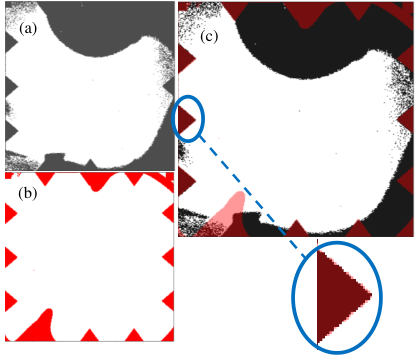
IV.1.1 Aligning IP and CR-39
In order to compare the IP and CR-39 to calculate the beamlet deflections, the images must be the same size and aligned to produce a 1:1 pixel comparison. The IP image has a higher resolution than the CR-39 and therefore must be cropped to isolate the image, eliminating extraneous boundary pixels beyond the frame, and resized to match the size of the corresponding CR-39. For the shots in which a jagged fiducial frame was used, the teeth from the IP and CR-39 images were isolated and the images overlapped to facilitate alignment (Fig. 3). The IP often required corrections including cropping, flipping, and/or rotating in order to achieve alignment with the corresponding CR-39. For shots where no jagged frame was present, we aligned the IP to the CR-39 based on the identified frame features, though this was more laborious and error prone due to the difficulty in identifying the features in all images, resulting in error of 1 pixel (therefore 0.9 T mm).

IV.1.2 Enhancing Images
To ease the process of finding beamlet locations, the images were enhanced to reduce the noise and improve the contrast (Fig. 4). First, a “box-car” filter with a size of 10x10 pixels (approximately the size of one beamlet) was applied to smooth the images. Then, another box-car filter of size 20x20 pixels was applied, and divided out from the smoothed image to normalize the fluence. The maximum and minimum pixel values within the mesh area of the image were used to define the final range of pixel values in the image; any pixel values in the image outside of this range were re-scaled. This ensures that the mesh is the area of the image with the maximum contrast.
As a figure of merit, we evaluated a “beamlet contrast” in the images, which we defined as the ratio of the maximum/mininum range of the beamlets to the rms of the sub-beamlet-scale noise (which can disrupt identifying the beamlet location). We found that this enhancement process results in a contrast improvement on the vacuum CR-39 images from 8 on the original to 60 on the enhanced.
An additional filter was applied to the IP image in order to further reduce the noise within each mesh opening, making the center of the mesh opening the location of the local extremum to aid in later processing of beamlet locations. The filter mimicks the shape of a beamlet, i.e. low values around the 2-pixel edges and high values in the 5x5 pixel center. This process results in an improvement of contrast for the IP from 2 on the original to 19 on the enhanced.
IV.2 Beamlet Detection
Once the contrast is improved, the images are rotated so that the rows are approximately horizontal, which allows an automated code to move along the row and search for the local extrema that correspond to beamlet centers. For ease of discussion, a second coordinate system in pixel units is defined in the frame of the image where is along the row and is along the column, i.e. in the rotated image is along the horizontal and is along the vertical.
This code takes user inputs that set the parameters for each row to be analyzed. These parameters include the indices of the beginning and end of the row in , the indices of the bottom and top of the row in , a beamlet spacing parameter, and row/column identifiers.


The start and end index values are averaged to set the initial -index for which the line-out along the row is drawn (Fig. 5a). This line-out is used to find the local extrema and therefore the initial index values of the beamlet coordinates in (Fig. 5b). For each -value, the pixels above and below the averaged -value are searched to find the extremum in the -direction (Fig. 5c). These and values set a preliminary coordinate for the beamlet that is then corrected and adjusted by searching around the initial point to find the actual local extremum (Fig. 5d).
The code also includes built-in checks that combat some common errors in the automatic location of the beamlets. These include checking the spacing of the beamlets in to prevent double-counting of beamlets, checking the distances between consecutive values to prevent jumping to a different row as can result in cases of large deflections, and repeatedly checking the pixels around each coordinate to ensure that the actual local extremum has been identified.
The final corrected coordinates for the analyzed row are saved into a data structure that records points by row and column index. These indices are defined using the fiducials on the nickel mesh including a keyhole cutout and glue dots over the mesh. These mark where row indices +1 and -1 and column index 0 are defined as shown in Fig. 6. The data structure is exported to a file. Once all coordinates have been found, they are transformed back to the initial unrotated, aligned images.
Despite the built-in checks, occasionally some points are not centered in the beamlets, so it remains important to spot check the beamlet locations against the raw data and apply manual adjustments when needed. In general, this entire process results in an error of 1 pixel for the beamlet locations. A completed IP and CR-39 after both the automatic code and manual adjustments is shown in Fig. 6.
IV.3 Line-Integrated Magnetic Field
Once corresponding IPs and CR-39s have been analyzed and the coordinates of the beamlets have been found, the path-integrated magnetic field can be calculated from the deflections. This process was completed for a calibration shot for the magnetic field in vacuum using the 14.7 MeV proton radiography image. We directly compare the CR-39 deflected beamlet coordinates with the undeflected beamlet coordinates on the IP; the spatial distribution of deflections is plotted in Fig. 7a. The deflections are then used to calculate the corresponding line-integrated magnetic field at each beamlet location using Eq. (6). The line-integrated magnetic field map is plotted in Fig. 7b and shows that in this highly-magnetized system, there is no area of zero magnetic field that can be used to provide a reference for analyzing the rest of the proton radiography image. This is where using the IP is necessary to provide reference positions. Finally, the magnitude of the path-integrated magnetic field for the three columns in the midplane between the MIFEDS (as outlined in Fig. 6) can be averaged and plotted as a function of position (Fig. 7d). The experimental data is also compared to the COMSOL Biot-Savart calculations of the magnetic field based on the coil geometry.
In order to evaluate the precision and efficiency of the new proposed technique using the IP, we compared the results to those obtained by an alternative method in which the reference undeflected beamlet positions were obtained from a CR-39 image of a separate vacuum shot with no magnetic field applied. The line-integrated magnetic field calculated using this technique is shown in Fig. 7c. Comparing both results, one can see that the PRAD/IP technique improves the accuracy of the magnetic field measurement by a factor of 4. The resulting error bar for both cases consists of the standard deviation of the path-integrated magnetic field values for the three central columns and the systematic error from the alignment of the data images. The alignment error for the PRAD/PRAD technique has two sources: the error from overlapping the two CR-39’s, 2 pixels, and the alignment error of mesh positioning in the experimental setup between the two separate shots that is estimated to be 25 m and yields 3 pixels in the detector plane. The PRAD/IP alignment error is 1 pixel due to the high resolution of the IP image. Then the total error is calculated as = . The PRAD/IP technique yields an average error of 1.2 T mm, while PRAD/PRAD yields an error of 5.7 T mm. The error bar for the new technique can be further improved by increasing the magnification, using the jagged frame to reduce alignment error, using other mesh periods, and using a mesh material of higher Z in order to enhance the contrast and therefore improve the beamlet identification in the automatic routine.


V Application to expanding plasma experiment
This technique was employed in an experiment at the OMEGA laser facility to study magnetic field dynamics in HED plasma in the regime including the magnetic field evolution over time, its diffusion, and potential anomalous transport processes. Expansion of the plasma into the background magnetic field locally expels the magnetic field and produces a diamagnetic cavity Dimonte and Wiley 1991; Ripin et al. 1993; Collette and Gekelman 2011; Niemann et al. 2013; Winske et al. 2019. The experimental setup is shown in Fig. 8. The coil geometry was identical to the calibration experiments discussed above; however, the MIFEDS current was increased to 34 kA. A plastic (CH) target was ablated to produce a plasma plume that flowed parallel to the field and into the region between the coils. The source target was 5 mm from the center of the diagnosed region. The laser energy on-target was 20 J in a 1 ns square pulse, the wavelength was 351 nm, and the laser-incidence angle on target was 33∘. The plasma was additionally diagnosed using Thomson scattering to measure plasma parameters, such as electron temperature and density.
As plasma expands into the magnetic field, it tends to push the magnetic field out of the volume it occupies leading to the formation of a diamagnetic cavity. This experiment was particularly focused on the study of diamagnetic cavity formation and evolution in time, which requires a precise magnetic field measurement. In Fig. 9 we show an example of the proton radiography data with 14.7 MeV protons (CR-39) and the corresponding x-ray image of the mesh (IP) obtained at 10 ns plasma expansion time. Fig. 9c shows the resulting line-integrated magnetic field evaluated along the midplane between the coils. One can clearly see the beginning of magnetic field cavitation by comparing the experimental data to the COMSOL calculation of the background magnetic field with no plasma. The CR-39 for this plasma shot shows an instance where a caustic (a locus of proton focusing and therefore beamlet overlap) interferes with the data Kugland et al. 2012; the three rows closest to one of the coils are cut off by the caustic, limiting the amount of data available for analysis.
VI Discussion and Conclusions
In conclusion, a novel technique of proton radiography was developed which simultaneously obtains a reference image of the undeflected beamlet locations by using an image plate x-ray detector in the detector stack. This technique allows absolute measurement of magnetic fields in systems which are globally magnetized and have no regions of zero magnetic field. Compared to a technique measuring the mesh pattern on surrogate experiments with and no plasma, the measurement is more accurate, largely owing to eliminating the uncertainty regarding reproducibility of the mesh construction and alignment between shots, and we estimate a factor 4 improvement for the present parameters. For efficient CR-39 and IP image processing we developed an automatic routine that allows for quick and accurate positioning of the beamlets. Using this method, we also have performed a characterization of the diamagnetic cavity formation and evolution in time in a >1 expanding plasma.
The data that support the findings of this study are available from the authors upon request.
VII Acknowledgements
This work was supported through DOE Laboratory Directed Research and Development. PJA, GS and AB were supported by the U.S. Department of Energy under Grant No. DE-NA0003868. PJA was also supported under Grant No. DE-NA0003960. The experiment was conducted at the Omega Laser Facility with the beam time through the Laboratory Basic Science under the auspices of the U.S. DOE/NNSA by the University of Rochester’s Laboratory for Laser Energetics under Contract DE-NA0003856.
References
- Li et al. (2006) C. K. Li, F. H. Séguin, J. A. Frenje, J. R. Rygg, R. D. Petrasso, R. P. J. Town, P. A. Amendt, S. P. Hatchett, O. L. Landen, A. J. Mackinnon, P. K. Patel, V. A. Smalyuk, T. C. Sangster, and J. P. Knauer, Physical Review Letters 97, 135003 (2006).
- Petrasso et al. (2009) R. D. Petrasso, C. K. Li, F. H. Seguin, J. R. Rygg, J. A. Frenje, R. Betti, J. P. Knauer, D. D. Meyerhofer, P. A. Amendt, D. H. Froula, O. L. Landen, P. K. Patel, J. S. Ross, and R. P. J. Town, Phys. Rev. Lett. 103, 085001 (2009).
- Yates et al. (1982) M. A. Yates, D. B. van Hulsteyn, H. Rutkowski, G. Kyrala, and J. U. Brackbill, Physical Review Letters 49, 1702 (1982).
- Fox et al. (2013) W. Fox, G. Fiksel, A. Bhattacharjee, P. Y. Chang, K. Germaschewski, S. X. Hu, and P. M. Nilson, Physical Review Letters 111, 225002 (2013).
- Huntington et al. (2015) C. M. Huntington, F. Fiuza, J. S. Ross, A. B. Zylstra, R. P. Drake, D. H. Froula, G. Gregori, N. L. Kugland, C. C. Kuranz, M. C. Levy, C. K. Li, J. Meinecke, T. Morita, R. Petrasso, C. Plechaty, B. A. Remington, D. D. Ryutov, Y. Sakawa, A. Spitkovsky, H. Takabe, and H. S. Park, Nature Physics 11, 173 (2015).
- Rygg et al. (2008) J. R. Rygg, F. H. Séguin, C. K. Li, J. A. Frenje, Manuel, R. D. Petrasso, R. Betti, J. A. Delettrez, O. V. Gotchev, J. P. Knauer, D. D. Meyerhofer, F. J. Marshall, C. Stoeckl, and W. Theobald, Science 319, 1223 (2008).
- Glenzer et al. (1999) S. H. Glenzer, W. E. Alley, K. G. Estabrook, J. S. De Groot, M. G. Haines, J. H. Hammer, J. P. Jadaud, B. J. MacGowan, J. D. Moody, W. Rozmus, L. J. Suter, T. L. Weiland, and E. A. Williams, Physics of Plasmas (1994-present) 6, 2117 (1999).
- Slutz et al. (2010) S. A. Slutz, M. C. Herrmann, R. A. Vesey, A. B. Sefkow, D. B. Sinars, D. C. Rovang, K. J. Peterson, and M. E. Cuneo, Physics of Plasmas 17, 056303 (2010).
- Sefkow et al. (2014) A. B. Sefkow, S. A. Slutz, J. M. Koning, M. M. Marinak, K. J. Peterson, D. B. Sinars, and R. A. Vesey, Physics of Plasmas 21, 072711 (2014).
- Nilson et al. (2006) P. M. Nilson, L. Willingale, M. C. Kaluza, C. Kamperidis, S. Minardi, M. S. Wei, P. Fernandes, M. Notley, S. Bandyopadhyay, M. Sherlock, R. J. Kingham, M. Tatarakis, Z. Najmudin, W. Rozmus, R. G. Evans, M. G. Haines, A. E. Dangor, and K. Krushelnick, Physical Review Letters 97, 255001 (2006).
- Li et al. (2007) C. K. Li, F. H. Séguin, J. A. Frenje, J. R. Rygg, R. D. Petrasso, R. P. J. Town, O. L. Landen, J. P. Knauer, and V. A. Smalyuk, Physical Review Letters 99, 055001 (2007).
- Fiksel et al. (2014) G. Fiksel, W. Fox, A. Bhattacharjee, D. H. Barnak, P. Y. Chang, K. Germaschewski, S. X. Hu, and P. M. Nilson, Physical Review Letters 113, 105003 (2014).
- Rosenberg et al. (2015a) M. J. Rosenberg, C. K. Li, W. Fox, A. B. Zylstra, C. Stoeckl, F. H. Séguin, J. A. Frenje, and R. D. Petrasso, Phys. Rev. Lett. 114, 205004 (2015a).
- Schaeffer et al. (2017) D. B. Schaeffer, W. Fox, D. Haberberger, G. Fiksel, A. Bhattacharjee, D. H. Barnak, S. X. Hu, and K. Germaschewski, Physical Review Letters 119 (2017), 10.1103/physrevlett.119.025001.
- Schaeffer et al. (2019) D. Schaeffer, W. Fox, R. Follett, G. Fiksel, C. Li, J. Matteucci, A. Bhattacharjee, and K. Germaschewski, Physical Review Letters 122 (2019), 10.1103/physrevlett.122.245001.
- Willingale et al. (2010) L. Willingale, A. G. R. Thomas, P. M. Nilson, M. C. Kaluza, S. Bandyopadhyay, A. E. Dangor, R. G. Evans, P. Fernandes, M. G. Haines, C. Kamperidis, R. J. Kingham, S. Minardi, M. Notley, C. P. Ridgers, W. Rozmus, M. Sherlock, M. Tatarakis, M. S. Wei, Z. Najmudin, and K. Krushelnick, Physical Review Letters 105, 095001 (2010).
- Rosenberg et al. (2015b) M. J. Rosenberg, C. K. Li, W. Fox, I. Igumenshchev, F. H. Séguin, R. P. J. Town, J. A. Frenje, C. Stoeckl, V. Glebov, and R. D. Petrasso, Nature Communications 6, 6190 (2015b).
- Kugland et al. (2012) N. L. Kugland, D. D. Ryutov, C. Plechaty, J. S. Ross, and H. S. Park, Review of Scientific Instruments 83, 101301 (2012).
- Séguin et al. (2003) F. H. Séguin, J. A. Frenje, C. K. Li, D. G. Hicks, S. Kurebayashi, J. R. Rygg, B.-E. Schwartz, R. D. Petrasso, S. Roberts, J. M. Soures, D. D. Meyerhofer, T. C. Sangster, J. P. Knauer, C. Sorce, V. Y. Glebov, C. Stoeckl, T. W. Phillips, R. J. Leeper, K. Fletcher, and S. Padalino, Review of Scientific Instruments 74, 975 (2003).
- Boehly et al. (1995) T. R. Boehly, R. S. Craxton, T. H. Hinterman, J. H. Kelly, T. J. Kessler, S. A. Kumpan, S. A. Letzring, R. L. McCrory, S. F. B. Morse, W. Seka, S. Skupsky, J. M. Soures, and C. P. Verdon, Review of Scientific Instruments 66, 508 (1995).
- Fiksel et al. (2015) G. Fiksel, A. Agliata, D. Barnak, G. Brent, P. Y. Chang, L. Folnsbee, G. Gates, D. Hasset, D. Lonobile, J. Magoon, D. Mastrosimone, M. J. Shoup, and R. Betti, Review of Scientific Instruments 86, 016105 (2015).
- Dimonte and Wiley (1991) G. Dimonte and L. G. Wiley, Physical Review Letters 67, 1755 (1991).
- Ripin et al. (1993) B. H. Ripin, J. D. Huba, E. A. McLean, C. K. Manka, T. Peyser, H. R. Burris, and J. Grun, Physics of Fluids B: Plasma Physics 5, 3491 (1993).
- Collette and Gekelman (2011) A. Collette and W. Gekelman, Physics of Plasmas 18, 055705 (2011).
- Niemann et al. (2013) C. Niemann, W. Gekelman, C. G. Constantin, E. T. Everson, D. B. Schaeffer, S. E. Clark, D. Winske, A. B. Zylstra, P. Pribyl, S. K. P. Tripathi, D. Larson, S. H. Glenzer, and A. S. Bondarenko, Physics of Plasmas 20, 012108 (2013).
- Winske et al. (2019) D. Winske, J. D. Huba, C. Niemann, and A. Le, Frontiers in Astronomy and Space Sciences 5, 51 (2019).