Dream to Explore: Adaptive Simulations for Autonomous Systems

Zahra Sheikhbahaee Affiliation: David R. Cheriton School of Computer Science Affiliation: University of Waterloo Affiliation: 200 University Avenue West Email: zsheikhb@uwaterloo.ca Dongshu Luo Affiliation: David R. Cheriton School of Computer Science Affiliation: University of Waterloo Affiliation: 200 University Avenue West Email: d33luo@uwaterloo.ca Blake VanBerlo Affiliation: David R. Cheriton School of Computer Science Affiliation: University of Waterloo Affiliation: 200 University Avenue West Email: bvanberlo@uwaterloo.ca S. Alex Yun Affiliation: David R. Cheriton School of Computer Science Affiliation: University of Waterloo Affiliation: 200 University Avenue West Email: alex.yun@uwaterloo.ca Adam Safron Affiliation: Johns Hopkins University School of Medicine Affiliation: 733 N Broadway, Baltimore Email: asafron1@jhmi.edu Jesse Hoey Affiliation: David R. Cheriton School of Computer Science Affiliation: University of Waterloo Affiliation: 200 University Avenue West Email: jhoey@cs.uwaterloo.ca

Abstract

One’s ability to learn a generative model of the world without supervision depends on the extent to which one can construct abstract knowledge representations that generalize across experiences. To this end, capturing an accurate statistical structure from observational data provides useful inductive biases that can be transferred to novel environments. Here, we tackle the problem of learning to control dynamical systems by applying Bayesian nonparametric methods, which is applied to solve visual servoing tasks. This is accomplished by first learning a state space representation, then inferring environmental dynamics and improving the policies through imagined future trajectories. Bayesian nonparametric models provide automatic model adaptation, which not only combats underfitting and overfitting, but also allows the model’s unbounded dimension to be both flexible and computationally tractable. By employing Gaussian processes to discover latent world dynamics, we mitigate common data efficiency issues observed in reinforcement learning and avoid introducing explicit model bias by describing the system’s dynamics. Our algorithm jointly learns a world model and policy by optimizing a variational lower bound of a log-likelihood with respect to the expected free energy minimization objective function. Finally, we compare the performance of our model with the state-of-the-art alternatives for continuous control tasks in simulated environments.

Keywords Bayesian Nonparametric $\cdot$ World Models $\cdot$ Reinforcement Learning $\cdot$ Unsupervised Learning $\cdot$ Latent Dynamics $\cdot$ Imagination

1 Introduction

In environments with high-dimensional observations, such as raw pixel visualizations, model-free reinforcement learning (RL) methods lack sample efficiency as observations must directly map to values or actions. Model-free methods are particularly undesirable for solving problems, where data collection is a challenge. Updating the policy or value function requires several environment interactions, leading to high sample complexity. Even after a long training period, the resultant policies lack the flexibility to adapt to novel tasks in the same environment [1].

In model-based planning, on the other hand, an agent learns the dynamics of an unknown environment, often requiring an order of magnitude less data than model-free counterparts. Furthermore, model-based RL has exhibited a promising capability to transfer to other tasks [2, 3]. Developing a generative model that is able to learn abstract spatial and temporal representations of the environment and utilizing it for policy learning with a simulated or more generalized version of reality can address the shortcomings of model-free RL algorithms [4]. An agent that is equipped with such a generative model of the world can synthesize alternative counterfactual simulations of possible future states in the environment and can perform planning on the rollouts of the probable scenarios [5]. A built-in perception-action cycle for such agents promotes predictive ability, which allows for abstract representations to be employed as the relevant information of the world for reasoning about the future. In this perspective, an action can be formulated as a computable objective function—namely, the path integral of variational free energy, which captures the expected evidence for pursuing a policy, given the world model of an agent [6].

An enduring goal of artificial intelligence (AI) is to design autonomous robots. The task of autonomous agent planning must be treated as a collection of three major components: (1) latent representation learning; (2) learning the dynamics of the environment (prediction); and (3) planning. These three components are combined as a single end-to-end training procedure. In practice, the collected high-dimensional observations are the consequence of latent processes present in the environment. By directly mapping raw sensory observations to a low-dimensional latent space, one can encode many of the high-level semantic features of the scene for the planning procedure [7]. These latent temporal patterns of momentary changes in the environment can be modelled by recurrent algorithms, creating internal memory representations of the dynamics of the world. We suggest that these stochastic hidden states may encapsulate uncertainty about the state variables, so facilitating the reconstruction of observations via inverse mapping.

Given that a plethora of sensory observations are generated from a multimodal prior distribution, Gaussian mixture priors are a reasonable choice to represent the multimodal structure present in the latent space data. A human’s ability to learn from a stream of novel data can be mimicked by allowing the number of parameters in the generative model to dynamically expand through the use of Bayesian nonparametric methods. Accommodating for the possibility of growth in model complexity enables adaptation in the number of cluster components of observational data [8].

Recurrent neural network (RNN) architectures can capture temporal dependences of the input data in their dynamical behaviour. Due to their inherent determinism, they cannot capture uncertainty in the latent space. Dynamic Bayesian networks (DBNs), such as the state space models, may have less expressive power compared to RNNs; however, they can represent both a transition function that describes the evolution of the internal latent state of the environment, as well as a projection from the hidden state to the final output [9]. Gaussian processes (GPs) delineate the probabilistic relations between the observed output data with respect to the inputs that consider the uncertainty-as being inherited from the data collection modality or the modelling assumptions- while also achieving good performances with smaller datasets [10]. GP models have remarkable predictive power in describing the nonlinear dynamical evolution of complex systems without being prone to overfitting. They are efficient in adapting to complex environments and they resemble a human’s ability to flexibly learn dynamics for planning in changing environments [11]. We consider a deep probabilistic autoregressive method by assuming a GP prior on the unknown transition function and on the observational model of an environment. We introduce a tractable variational approximation to compute latent state posterior and temporal correlations. This approach entails back propagation of errors back through time, chained from the predicted back to the observed output of the system [12].

Structural (inductive) biases can potentially enhance (or hinder) the performance of model-based RL algorithms, compared to their model-free counterparts. Learning the transition probabilities of the environment and incorporating the optimization of the value functions in policy selection can embrace the best of the model-free and model-based RL methods [13].

We tackle the planning problem for autonomous systems from the perspective of probabilistic inference and learning, and assess our method in partially observable environments. Our contributions consist of three parts:

1.

We construct an informal mental representation of the world, which can be used for planning as a kind of value-guided construal [11]. We employ a variational autoencoder with an infinite mixture of Gaussian priors on the abstract environmental representation to garner the intricate structure of multimodal (visual) sensory inputs. We employ a Bayesian nonparametric algorithm that is rooted in the foundations of how a rational learners adaptively categorizes representations of the observed stimuli in a potentially unbounded number of clusters [14].
2.

The agent uses a recurrent Gaussian process (RGP) model that acts as working memory to imagine the counterfactual policies. This structure captures the propagating uncertainty across time. Further, as a Bayesian nonparametric approach, GP can flexibly model uncertainty by inferring distributions over functions. RGP offers unique meta-learning abilities that enable the learning of a stochastic processes efficiently from limited observations, while generalizing over multiple tasks. This ingredient of our model captures the ordering and recurrent features from observed sequences of data. Using imagination, one can plan on counterfactual trajectories with a learned world model. These imagined experiences can use encoded prior knowledge to unfold the evolution of possible action-conditioned states of the world driven by the encoded prior knowledge [15]. This is functionally similar to the default mode network of the brain, which is responsible for internally oriented mental processes for deliberate, goal-directed tasks. This core functional network can also include episodic memory retrieval and constructive mental simulations by taking into account environmental dynamics [16].
3.

We consider control as an inference problem [17]; wherein we derive he Bellman function from an expected free energy objective functional over augmented data, which we generate from future rollouts of potential actions. Our hybrid model uses a stochastic actor-critic algorithm, jointly optimizing the value function and policy. In this construct, the policy network is referred to as the actor, while the value function as the critic.

2 Related Work

2.1 Model-Free Reinforcement Learning

Effective policies can be learned without explicitly constructing a dynamical model of the world [18]. The soft actor-critic algorithm was proposed to enhance sample efficiency and reduce the sensitivity of on-policy methods to changes in hyperparameters by introducing a maximum entropy term to the standard RL objective function, as well as an off-policy actor-critic method for a continuous state-action spaces [19]. A policy evaluation network (i.e. critic), which estimates the value function for a given policy, is optimized in tandem with a stochastically updated policy network (i.e. actor).

Lee et al. [20] addressed the challenges of learning policies in high-dimensional observation spaces by introducing an algorithm to separately learn abstract representations and deploy RL models in the learned latent space. They derived a Bellman backup formulation of control (as inference) and employed amortized variational inference to train a Markovian model using the actor-critic method.

In the probabilistic inference formulation of the RL problem, the variational posterior of trajectories can be computed, conditioned on a desired outcomes [21, 22]. An expectation-maximization (EM) style algorithm was proposed wherein the E-step the dynamics of the environment computes the value function (critic update) and the variational policy (actor update) [23]. In the M-step, the baseline policy is updated given the variational distribution of policy and the transition function.

2.2 Model-Based Reinforcement Learning

Model-based algorithms have addressed the sample efficiency challenge in deep RL by leveraging simple function approximators or probabilistic methods. That said, model bias can induce worse asymptotic performance under conditions of high sample complexity. Zhang et al. [24] jointly learned the global dynamics, cost models, and abstract representations from high-resolution images. They employed simpler linear models to allow the direction of gradients to improve the local policies. Similarly, by using deep spatial autoencoders, low-dimensional state representations can be learned from visual sensory data in a supervised fashion to optimize linear-Gaussian controllers, which was shown to find optimal trajectories for agents when combined with a guided policy search [25]. The Deep Planning Network (PlaNet) was proposed to learn the dynamics of compact representations of world dynamics, strengthening long-term predictions with a latent overshooting procedure in which multiple-step predictions are afforded in latent space [2].

While many model-based methods suffer from model bias, probabilistic inference for learning control (PILCO) addresses this shortcoming by learning a probabilistic dynamics model. PILCO utilizes GPs to explicitly incorporate model uncertainty and estimates the policy gradients to find locally optimal solutions for control problems [26]. Despite its efficacy for some tasks, this method suffers in environments with high-dimensional spaces or discernible nonlinear dynamics. To improve performance under conditions of high sample complexity, the union of model-based controllers (such as model predictive control) with a policy gradient algorithm for model-free fine-tuning has achieved high performance for some challenging problems [27].

2.3 Counterfactual Planning

World models can be built by learning both the latent representations of temporal and spatial sensory observations [5, 2]. The application of RNNs entails prediction on how the world evolves based on previous memories [28]. Of note is Ha & Schmidhuber’s work, in which training took place inside hallucinated dreams generated by an agent’s own world model, utilizing a low-parameter controller. Also significant is the DreamerV2 model, in which an actor-critic algorithm leveraged a generative world model to learn optimal behaviours, achieving human-level performance on Atari benchmarks [4]. Further, these agents were able to learn policies using data augmentation from imagined dynamics, enabling adaptation to novel environments [29].

3 Preliminaries

We study autonomous systems in a partially observable Markov decision process (POMDP) setting. We define a tuple $\mathcal{M}=(X,Z,A,P,r,\gamma)$ , where $x_{t}\in X$ and $z_{t}\in Z$ are observations and states, respectively. $A$ is a set of continuous actions, $P$ delineates the transition probabilities $P(z_{t+1}|z_{t},a_{t})$ , $r:Z\times A\rightarrow\mathbb{R}$ defines the reward function, and $\gamma$ is a discount factor to guarantee the finite sum of expected rewards for an infinite horizon. The goal of conventional RL algorithm is to learn some policy, $\pi(a_{t}|z_{t})$ under a trajectory distribution $\rho_{\pi}$ , which seeks to maximize the sum of future rewards.

3.1 Learning the World Model with an Infinite Gaussian Mixture Variational Autoencoder

Figure 1: The generative model, with an infinite mixture of Gaussians as the prior for the variational autoencoder: We use a stick-breaking construction and learn the low-dimensional representation of the environment. Here

X_{t}

is environmental observation and

z_{t}

is the continuous latent space.

Impeccable perception is a key quality that an autonomous agent must possess to have successful interactions with the world. In our model, the latent representations of the sensory data are generated by considering an infinite mixture-of-Gaussians prior for learning a reliable representation of the world. Such a method offers immense modelling flexibility, structured interpretability, and avoids the loss of rich semantics present in visual data [30]. The assumption of a single Gaussian, despite imposing strong constraints on the true posterior (which is often multimodal), can lead to poor model performance.

The Dirichlet process (DP) is a prior probability distribution to capture nonparametric Bayesian problems. Construction of the DP using a stick-breaking process can be introduced as an infinite sum of an atomic distribution [31]. The DP comprises a concentration parameter $\alpha\in\mathbb{R}^{+}$ , and a probability measure $G_{0}$ , which is referred to as the base measure, where $G\sim\mathrm{DP}(\alpha,G_{0})$ . The stick-breaking representation of $G$ is given by

\begin{split}\theta_{i}(\boldsymbol{\nu})&=\nu_{i}\prod_{j=1}^{i-1}(1-\nu_{j})\\ G&=\sum_{i=1}^{\infty}\theta_{i}(\boldsymbol{\nu})\;\delta_{\psi_{i}}\end{split}

(1)

where $\theta_{i}(\boldsymbol{\nu})$ is the infinite vector of mixing proportions and $\psi_{1},\psi_{2},..$ defines the atoms representing the mixture components [32].

The perception in our model is designed by considering a flexible prior to accommodate many different structures in the world, while preferring to expand parsimoniously. The dimension of latent representation can grow adaptively once the agent encounters novel observations. The generative process that predicts future observations given the perceptual world model of an agent can be defined as

\begin{split}x_{t}\;|\;z_{t};\phi&\sim\mathscr{N}\Big(\mu,\mathrm{diag}(\sigma^{2})\Big)\\ \mathbf{z}_{t}\;|\;c_{t},w_{t}&\sim\prod_{n=1}^{N}\prod_{k=1}^{\infty}\mathscr{N}\Big(\mu_{c^{k}_{t}}(w_{t};\beta),\mathrm{diag}\big(\sigma^{2}_{c^{k}_{t}}(w_{t};\beta)\big)\Big)^{c_{t}^{nk}}\\ w_{t}&\sim\mathscr{N}\Big(\boldsymbol{0},\mathbb{I}\Big)\\ c_{t}\;|\;\boldsymbol{\theta_{t}}&\sim\mathrm{Cat}\Big(\theta(\boldsymbol{\nu})\Big)\\ \nu_{i}&\sim\mathrm{Beta}(1,\alpha)\end{split}

(2)

where $\theta_{k}$ is the prior mixing weights for cluster $c_{t}$ ( $\sum_{k=1}\theta^{K}=1$ ), $\mu_{c}$ and $\sigma_{c}^{2}$ are the mean and the variance of the Gaussian distribution corresponding to cluster $c_{t}$ in the latent space, and observation $\boldsymbol{x}$ is a neural network whose input is $z$ and is parametrized by $\phi$ .

The prior distribution over the latent space $\mathbf{z}|w$ is a Gaussian mixture model whose means and variances are specified by another neural network, parametrized by $\beta$ with input variable $w$ , which can capture more subtle properties of data in the latent space such as “style” [33]. We assume the mean-field variational family to approximate the posterior distributions. The variational lower bound for finding the abstract latent states of the environment can be written as

\begin{split}\mathscr{L}_{\mathrm{iGMMVAE}}&=\underbrace{\mathbb{E}_{q(z_{t}|x_{t})}\Big[\log p(x_{t}|z_{t})\Big]}_{\text{the reconstruction term}}-\mathrm{D}_{\mathrm{KL}}\Big[q(w_{t}|x_{t})||p(w_{t})\Big]\\ &-\mathbb{E}_{p(c_{t}|z_{t},w_{t})q(w_{t}|x_{t})}\Bigg[\mathrm{D}_{\mathrm{KL}}\Big[q(z_{t}|x_{t})||p(z_{t}|c_{t},w_{t})\Big]\Bigg]\\ &-\mathbb{E}_{q(\theta_{t}|x_{t})q(w_{t}|x_{t})q(z_{t}|x_{t})}\Bigg[\mathrm{D}_{\mathrm{KL}}\Big[p(c_{t}|z_{t},w_{t})||p(c_{t}|\theta_{t})\Big]\Bigg]\\ &-\mathrm{D}_{\mathrm{KL}}\Big[q(\theta_{t}|x_{t})||p(\theta_{t}|\alpha)\Big]\end{split}

(3)

The reconstruction term in this objective function encourages the decoder to reconstruct the data when employing samples from the latent distribution $z$ and the KL divergence terms can be viewed as regularization terms. Following the assumption in [33], the posterior distribution of the indicator variable of each cluster can be obtained by

\begin{split}q_{\phi}(c_{t}|x_{t})=p_{\beta}(c_{t,j}=1|z_{t},w_{t})=\frac{\pi_{j}\mathscr{N}\Big(\mu_{j},\mathrm{diag}(\sigma_{j}^{2})\Big)}{\sum_{k=1}^{\infty}\pi_{j}\mathscr{N}\Big(\mu_{k},\mathrm{diag}(\sigma_{k}^{2})\Big)}\end{split}

(4)

We employ the Gumbel-Softmax distribution as categorical prior which is differentiable and allows us to backpropagate through $c$ [34].

We compute the final KL divergence term in Equation (4) between the Kumaraswamy and the Beta distribution, which has a closed-form [35]. The Kumaraswamy distribution $q(\nu|x)$ is considered as a doubly bounded continuous distribution which resembles the Beta distribution when its hyperparameters are equal to one and we employed this distribution to use its fully differentiable property for backpropagation.

3.2 Gaussian Process State-Space Model

An agent must learn the dynamics of the environments for planning, which can be transferable to different tasks. The world model is the compressed sequence of observations, which can predict the consequences of actions. A recurrent structure acts as internal memory to capture the spatial and temporal patterns in the environment. We apply an autoregressive structure on the latent states of world which incorporates GP priors to learn the uncertainty present in data as well as the nonlinearity in the transition dynamics, reward, and controller functions. We introduce a variational inference procedure to integrate GP into an RNN architecture and use it for counterfactual action planning.

Figure 2: The graphical model of Deep GP-recurrent which comprises of

2H+1

layers for transition, reward (emission) and controller layers. The transition, observation (

f^{(.)}

) as well as controller (

g^{(.)}

) functions have Gaussian process priors.

3.2.1 Recurrent Gaussian Processes

For mental simulation, one requires a predictive map of the environment. An agent’s decision-making process consists of combining the multi-step abstract representation of the world with the evaluation of the reward for the given trajectory. A similar method is the successor representation-Dyna oeuvre, where low-dimensional representations are stored in the temporal context model of memory, enabling one to learn flexible affiliated reward dynamics via offline episodic replay [36, 37]. With this idea as inspiration, we employ the recurrent GP model proposed by [38], which is similar to RNNs.

We represent the deep structure of our probabilistic recurrent state-space model by considering $H$ time steps for the planning horizon, which necessitates the inclusion of a hidden layer for each transition function in our construct.

\begin{split}z_{i}^{(h)}&=f^{(h)}\big(\hat{z}_{i}^{(h)}\big)+\epsilon_{i,f}^{(h)},\;\;\mathbf{f}^{(h)}\sim\mathscr{N}\Big(\boldsymbol{0},\boldsymbol{K}_{f}^{(h)}\Big),\;\;1\leq h\leq H\\ a_{i}^{(h)}&=g^{(h)}\big(\hat{w}_{i}^{(h)}\big)+\epsilon_{i,g}^{(h)},\;\;\mathbf{g}^{(h)}\sim\mathscr{N}\Big(\boldsymbol{0},\boldsymbol{K}_{g}^{(h)}\Big),\;\;1\leq h\leq H\\ r_{i}&=f^{(H+1)}\big(\hat{z}_{i}^{(H+1)}\big)+\epsilon_{i,f}^{(H+1)},\;\;\mathbf{f}^{(H+1)}\sim\mathscr{N}\Big(\boldsymbol{0},\boldsymbol{K}_{f}^{(H+1)}\Big)\end{split}

(5)

Above, $\epsilon^{(h)}_{i,f}$ is the transition noise and $\epsilon_{i,g}^{(h)}$ is the noise present in the controller function. The noise in each layer is delineated by $\epsilon_{i}^{(h)}\sim\mathscr{N}(0,\sigma_{h}^{2})$ . We define that the GP priors have zero mean and $\boldsymbol{K}_{f}^{(h)}$ where $\boldsymbol{K}_{g}^{(h)}$ are covariance matrices with entries $K_{f}^{ij}=k(z_{i},z_{j})$ – usually radial basis function (RBF) kernels. The inputs for each layer are given by $\displaystyle\hat{z}_{i}^{(h)}=\left\{\begin{array}[]{ll}\big[\bar{z}_{i-1}^{(1)},\bar{x}_{i-1}]^{T}=\Big[\big[z_{i-1}^{(1)},..,z_{i-M}^{(1)}\big],\big[x_{i-1},..,x_{i-M_{x}}\big]\Big]^{T},\\ &h=1\\ \big[\bar{z}_{i-1}^{(h)},\bar{z}_{i}^{(h-1)}]^{T}=\Big[\big[z_{i-1}^{(h)},..,z_{i-M}^{(h)}\big],\big[z_{i}^{(h-1)},..,z_{i-M+1}^{(h-1)}\big],\big[a_{i-1}^{(h-1)},..,a_{i-L_{a}}^{(h-1)}\big]\Big]^{T},\\ &1<h\leq H\\ \bar{w}_{i}^{(h)}=\big[z_{i-1}^{(h)},..,z_{i-M+1}^{(h)}\big]^{T},\\ &1<h\leq H\\ \bar{z}_{i}^{(h)}=\Big[\big[z_{i-1}^{(H)},..,z_{i-M+1}^{(H)}\big],\big[a_{i-1}^{(H)},..,a_{i-L_{a}}^{(H)}\big]\Big]^{T},\\ &h=H+1\end{array}\right.$ where $M$ is the number of lagging steps for the latent dynamical variable $z_{i}^{(h)}$ , the lag orders $M_{x}$ is chosen as the exogenous inputs $x_{i}^{(h)}$ (i.e. action or actions or both), $\hat{z}_{i}^{(h)}$ is the endogenous input of each layer, and $\bar{w}_{i}$ is the input of a single layer which acts as a controller to determine the course of actions. The vector $\bar{z}_{i}^{(h)}$ expresses the autoregressive latent state related to the layer $h$ in the instant $i$ . The key difference between this structure with previous works is the inclusion of separate functions to model the controller in each step with its own independent noise model [39, 10].

We exploit variational inference to obtain analytical forms for the posterior of $f$ and $g$ functions and compute a lower bound for the marginal likelihood of $\mathbf{f}$ . We follow Titsias’s [40] variational sparse GP framework and we introduce $\zeta$ and $\lambda$ as inducing points. The joint distribution of all the variables in the generative process is

\begin{split}p&\Big(r,a,f^{H+1},\zeta^{(H+1)},\big\{z^{h},f^{h},\zeta^{h},g^{h},\lambda^{h}\big\}|_{h=1}^{H}\Big)=\\ &\prod_{i=M+1}^{N}p\big(r_{i}|f_{i}^{(H+1)}\big)p\big(f_{i}^{(H+1)}|\zeta^{(H+1)},\hat{z}_{i}^{(H)}\big)\\ &\prod_{h=1}^{H}p\big(z_{i}^{(h)}|f_{i}^{(h)}\big)p\big(f_{i}^{(h)}|\zeta^{(h)},\hat{z}_{i}^{(h)}\big)p\big(a_{i}^{(h)}|g_{i}^{(h)}\big)p\big(g_{i}^{(h)}|\lambda^{(h)},\hat{z}_{i}^{(h)}\big)\\ &\prod_{h=1}^{(H+1)}p\big(\zeta^{(h)}\big)\prod_{h=1}^{(H)}p\big(\lambda^{(h)}\big)\prod_{i=1}^{M}\prod_{h=1}^{H}p\big(z_{i}^{(h)}\big).\end{split}

(6)

If we consider the mean-field approximation, then the variational posterior distribution $Q$ is given by

\begin{split}Q=&\Bigg(\prod_{h=1}^{H}q\big(z^{(h)}\big)\Bigg)\Bigg(\prod_{h=1}^{H+1}q\big(\zeta^{(h)}\big)\Bigg)\Bigg(\prod_{h=1}^{H+1}\prod_{i=L+1}^{N}p\big(f_{i}^{(h)}|\zeta^{(h)},\hat{z}_{i}^{(h)}\big)\Bigg)\\ &\Bigg(\prod_{h=1}^{H}q\big(\lambda^{(h)}\big)\Bigg)\Bigg(\prod_{h=1}^{H}\prod_{i=L+1}^{N}p\big(g_{i}^{(h)}|\lambda^{(h)},\hat{z}_{i}^{(h)}\big)\Bigg)\end{split}

(7)

where inducing points $\zeta^{(h)}$ in each layer $h$ can be parametrized as a distribution $q(\zeta^{(h)})=\mathcal{N}\Big(\zeta^{(h)}|\mathbf{m}^{(h)},\mathbf{S}^{(h)}\Big)$ where $h\in\{1,...,H+1\}$ for obtaining a non-collapsed bound which is suitable for large datasets.

Following the mean-field approximation, the distribution of the latent variable is defined as $q(\boldsymbol{z}^{(h)})=\prod_{i=1}^{N}\mathscr{N}\big(z_{i}^{(h)}|\mu_{i}^{(h)},\beta_{i}^{(h)}\big)$ , where $\mu^{(h)}$ and $\beta^{(h)}$ are variational parameters. We utilize multilayer perceptron network as recognition models for the variational parameters [10, 41]. Therefore, we have

\begin{split}\mu_{i}^{(h)}&=\psi_{\mu,2}\Big(\mathbf{W}^{(h)T}_{\mu,2}\psi_{\mu,1}\big(\mathbf{W}^{(h)}_{\mu,1}\hat{z}_{i-1}^{(h)}\big)\Big)\\ \beta_{i}^{(h)}&=\psi_{\beta,2}\Big(\mathbf{W}^{(h)T}_{\beta,2}\psi_{\beta,1}\big(\mathbf{W}^{(h)}_{\beta,1}\hat{z}_{i-1}^{(h)}\big)\Big)\end{split}

(8)

where $\mathbf{W}^{(h)T}_{\mu,l}$ , $\mathbf{W}^{(h)T}_{\beta,l}$ , $l\in\{1,2\}$ are the weights of neural networks ad $\psi_{\mu,l}\Big(.\Big)$ and $\psi_{\beta,l}\Big(.\Big)$ express element-wise activation functions. For $\beta_{i}^{(h)}$ the output of the network must be non-negative values. The lower bound of log marginal likelihood is defined as

\begin{split}\mathscr{L}_{\mathrm{RGP}}&=\\ \log p\big(\boldsymbol{r},\boldsymbol{a}\big)&\geq\sum_{i=1}^{N}\Bigg\{\sum_{h=1}^{H}\underbrace{\Big\langle p\big(f_{i}^{(h)}|\zeta^{(h)},\hat{z}_{i}^{(h)}\big)\log p\big(z_{i}^{(h)}|f_{i}^{(h)}\big)\Big\rangle_{q(\boldsymbol{z})q(\boldsymbol{\zeta})}}_{\mathscr{L}_{i}^{(h)}}\\ &+\underbrace{\Big\langle p\big(f_{i}^{(H+1)}|\zeta^{(H+1)},\hat{z}_{i}^{(H)}\big)\log p\big(r_{i}|f_{i}^{(H+1)}\big)\Big\rangle_{q(\boldsymbol{z})q(\boldsymbol{\zeta})}}_{\mathscr{L}_{i}^{(H+1)}}\Bigg\}\\ &+\sum_{i=1}^{N}\sum_{h=1}^{H}\underbrace{\Big\langle p\big(g_{i}^{(h)}|\lambda^{(h)},\hat{z}_{i}^{(h)}\big)\log p\big(a_{i}^{(h)}|g_{i}^{(h)}\big)\Big\rangle_{q(\boldsymbol{z})q(\boldsymbol{\lambda})}}_{\mathscr{J}_{i}^{(h)}}\\ &-\sum_{i=1}^{N}\sum_{h=1}^{H}\underbrace{\Big\langle\log q(z_{i}^{(h)})\Big\rangle_{q(\boldsymbol{z})}}_{\mathscr{H}_{i}^{(h)}}+\sum_{i=1}^{L}\sum_{h=1}^{H}\underbrace{\Big\langle\log p(z_{i}^{(h)})\Big\rangle_{q(\boldsymbol{z})}}_{\mathscr{L}_{0i}^{(h)}}\\ &-\sum_{h=1}^{H+1}\mathrm{KL}\Big[q(\zeta^{(h)})||p(\zeta^{(h)})\Big]-\sum_{h=1}^{H}\mathrm{KL}\Big[q(\lambda^{(h)})||p(\lambda^{(h)})\Big]\end{split}

(9)

where $\mathscr{H}_{i}^{h}|_{h=1}^{H}$ contains the entropy terms and $\mathscr{L}_{0i}^{(h)}$ expresses the initial conditions imposed by computing the expected value of the priors $p\big(z_{i}^{(h)}\big)=\mathscr{N}\bigg(z_{i}^{(h)}|\mu_{0i}^{(h)},\beta_{0i}^{(h)}\bigg)$ which can be optimized with the variational parameters or they can be fixed, e.g., $\mu_{0i}^{(h)}=0$ and $\beta_{0i}^{(h)}=1$ . The terms $\mathscr{L}_{i}^{(h)}|_{h=1}^{H}$ include learning the transition dynamics, the $\mathscr{L}_{i}^{(H)}$ comprises the reward in the environment and $\mathscr{J}_{i}^{(h)}$ is responsible for inferring the controller functions at each time step. Here we can compute $p\big(f_{i}^{(h)}|\zeta^{(h)},\hat{z}_{i}^{(h)}\big)=\mathscr{N}\big(\overbrace{\mathbf{K}_{z\zeta}^{(h)}(\mathbf{K}_{\zeta}^{(h)})^{-1}\zeta^{(h)}}^{\boldsymbol{b}_{f}^{(h)}},\overbrace{\mathbf{K}_{z}^{(h)}-\mathbf{K}_{z\zeta}^{(h)}(\mathbf{K}_{\zeta}^{(h)})^{-1}\mathbf{K}_{\zeta z}^{(h)}}^{\boldsymbol{\Sigma}_{f}^{(h)}}\big)$ and similarly we have $p\big(g_{i}^{(h)}|\lambda^{(h)},\hat{z}_{i}^{(h)}\big)=\mathscr{N}\big(\mathbf{K}_{z\lambda}^{(h)}(\mathbf{K}_{\lambda}^{(h)})^{-1}\lambda^{(h)},\mathbf{K}_{z}^{(h)}-\mathbf{K}_{z\lambda}^{(h)}(\mathbf{K}_{\lambda}^{(h)})^{-1}\mathbf{K}_{\lambda z}^{(h)}\big)$ .

The derivation of different components of the bound which are given in eq. (9) was provided inside section (7) of the supplementary material.

In order to employ the model for a large dataset, we can consider a mini-batch $\mathcal{B}$ , which can be a set of B sequential indexes sampled from the training data. We can perform stochastic optimization over mini-batches on a non-collapsed variational bound. Although this structure is closely related to that of traditional RNNs, it takes into account the stochasticity of the data and the environment.

The loss functions for the infinite Gaussian Mixture VAE, $\mathscr{L}_{\mathrm{iGMMVAE}}$ , and for the deep recurrent Gaussian Process, $\mathscr{L}_{\mathrm{RGP}}$ , are optimized jointly using the Adam optimiser to learn the world model.

4 Planning

Similar to Hafner et al. [2], we can use model-predictive control for planning based on new observations. That is, we can replan at each step by simply utilizing the RGP algorithm for a limited time horizon or trajectory rollouts. However, we combine both model-based and model-free methods to increase robustness of our model to imperfections and improve sample efficiency [1, 42]. The RGP serves as a predictive model of the future and generates imaginative rollouts a few steps in the future with different random initializations. The forward predictions contain a sequence of $\{z_{t},a_{t},r_{t}\}_{t=1}^{H}$ in the latent space and are fed to a stochastic latent actor-critic to compute the optimal policy and estimate the value function.

We begin by considering planning as inference and we formalize it in terms of the expected free energy [43, 21]. We can derive the the Bellman backup as a recursive logic over the agent’s trajectory and we define the binary variable $\mathscr{O}_{t}$ which denotes that time step $t$ is optimal given $p(\mathscr{O}_{t}=1|z_{t},a_{t})=\exp(r(z_{t},a_{t}))$ . First, we start with the evidence lower-bound (ELBO) of the log-likelihood function

$\begin{aligned} &\mathcal{G}(a_{\tau},z_{\tau})\\ &=\mathbb{E}_{q_{\phi}(a_{\tau:T}|z_{\tau:T})q_{\phi}(z_{\tau:T}|a_{\tau:T})}\Bigg[\log\bigg(\prod_{t=\tau}^{T}\Big[p_{\theta}(z_{t}|a_{t-1},z_{t-1})p_{\theta}(a_{t}|z_{t})\Big]\\ &\exp\Big[\eta\;\sum_{t=\tau}^{T}r(z_{t},a_{t})\Big]\Bigg)-\log\Bigg(\prod_{t=\tau}^{T}q_{\phi}\big(a_{t}|z_{t}\big)\;q_{\phi}\big(z_{t+1}|a_{t},z_{t}\big)\Bigg)\Bigg]\\ &=\underbrace{\sum_{t=\tau}^{T}\mathbb{E}_{q_{\phi}\big(z_{t+1}|a_{t},z_{t}\big)}\Bigg[\eta\mathbb{E}_{q_{\phi}\big(a_{t}|z_{t}\big)}\Big[r\big(z_{t},a_{t}\big)\Big]-\mathrm{D}_{\mathrm{KL}}\Big[q_{\phi}(a_{t}|z_{t})\big|\big|p_{\theta}(a_{t}|z_{t})\Big]\Bigg]}_{\text{policy objective term}}\\ &-\underbrace{\mathbb{E}_{q_{\phi}\big(a_{t}|z_{t}\big)}\Bigg[\mathrm{D}_{\mathrm{KL}}\Big[q_{\phi}\big(z_{t+1}|a_{t},z_{t}\big)\big|\big|p_{\theta}\big(z_{t+1}|a_{t},z_{t}\big)\Big]\Bigg]}_{\text{dynamic objective term}}\end{aligned}$

(10)

where $\eta$ is a temperature parameter which identifies the relative importance of the entropy term against the reward in the environment, affecting the degree of stochasticity in the optimal policy. The third term is the cross-entropy between the posterior dynamics $p(z_{t+1}|a_{t},z_{t},\mathscr{O}_{1:T})$ and the true dynamics $p(z_{t+1}|a_{t},z_{t})$ . In our setting, the agent’s goal is to find a policy which maximizes the expected return by estimating the probability of a system trajectory under each policy computed in the latent space.

\fname@algorithm Dream to Explore

p(z_{t}|z_{t-1},a_{t-1})

\triangleright

Transition model

P(x_{t}|z_{t})

\triangleright

Observation model

P(r_{t}|z_{t},a_{t})

\triangleright

Reward model

5: Initialize dataset

D

with

\mathscr{M}

random seed episodes

6: while not converged do

7: for update step

z=1,...,R

8: Draw chunks

\Big\{\Big[a_{t},r_{t},z_{t}\Big]_{k=1}^{{\mathrm{Chunk}}}\Big\}_{i=1}^{\mathrm{Batch}}

9: Run recurrent GP model

10: Compute

\mathscr{L}_{\mathrm{iGMMVAE}}+\mathscr{L}_{\mathrm{RGP}}

and update world model parameters

11: end for

12:

o_{1}\leftarrow env.reset()

13: for time step

t=1,...,T

14:

a_{t}\leftarrow

Planner(

o_{t}

, iGMMVAE, RGP)

15:

o_{t+1},r_{t}\leftarrow env.step(a_{t})

16: end for

17:

D\leftarrow D

\cup

\Big\{(o_{t},a_{t},r_{t})_{t=1}^{T},o_{T+1}\Big\}

18: for each gradient step do

19:

\phi\leftarrow\phi-\lambda_{\pi}\nabla_{\phi}J_{\pi}(\phi)

\triangleright

Update Actor

20:

\theta\leftarrow\theta-\lambda_{Q}\nabla_{Q}J_{Q}(\theta)

21:

\psi\leftarrow\psi-\lambda_{V}\nabla_{\psi}J_{V}(\psi)

\triangleright

Update Critic

22: end for

23: end while

We can rewrite the above RL objective in terms of backward messages to obtain standard Bellman-like operator [23] which is provided in the supplementary materials section (8).

By passing messages backward through time, we can minimize the soft Bellman residual, while the KL divergence term as a regularizer becomes minimized when two distributions become as close as possible to each other. The goal is to update the policy in order to be optimized with respect to the critic; therefore, the optimal policy minimizes the KL divergence in the last line of above equation [20].For the policy improvement step, we optimize the variational policy distribution by minimizing the following loss function

\begin{split}J_{\pi}(\phi)=\mathbb{E}_{z_{\tau+1}\sim P(.|z_{\tau},a_{\tau})}&\Bigg[\mathbb{E}_{a\sim P(.|z_{\tau+1})}\bigg\{\log\frac{q(a_{\tau+1}|z_{\tau+1})}{p(a_{\tau+1}|z_{\tau+1})}\\ &-Q(z_{\tau+1},a_{\tau+1})+V(z_{\tau+1})\bigg\}\Bigg]\end{split}

(11)

where the soft value function can be optimized using the following loss objective [23]:

\begin{split}J_{V}(\psi)=\mathbb{E}_{z_{\tau+1}\sim P(.|z_{\tau},a_{\tau})}&\Bigg[\frac{1}{2}\bigg\{V(z_{\tau+1})-\mathbb{E}_{q_{\phi}(a_{\tau+1}|z_{\tau+1})}\bigg(Q(z_{\tau+1},a_{\tau+1})\\ &-\log\frac{q_{\phi}(a_{\tau+1}|z_{\tau+1})}{p(a_{\tau+1}|z_{\tau+1})}\\ &-\log\frac{q(z_{\tau+2}|a_{\tau+1},z_{\tau+1})}{p(z_{\tau+2}|a_{\tau+1},z_{\tau+1})}\bigg)\bigg\}^{2}\Bigg]\end{split}

(12)

The second and the third terms in the objective function guarantee incorporation of risk-seeking policies and improve exploration by promoting diverse behaviors.

Similar to [20], we minimize the temporal difference error using the critic network with the following loss objective:

\begin{split}J_{Q}(\theta)&=\mathbb{E}_{z_{t}\sim q(.|z_{t-1},a_{t-1}),a_{t}\sim q(.|z_{t})}\Bigg[\frac{1}{2}\Bigg\{\;Q(z_{t},a_{t})-\Bigg(\eta\;r(a_{t},z_{t})\\ &+\gamma\log\mathbb{E}_{z_{t+1}\sim q(z_{t+1}|z_{t},a_{t})}\Big[\exp\Big(V(z_{t+1})\Big)\Big]\Bigg)\;\Bigg\}^{2}\Bigg]\end{split}

(13)

separate policy and value function networks. Dream to Explore is outlined in Algorithm (1).

Haarnoja et al. [19] assumed that value functions can be modelled as neural networks, with the policy as a Gaussian with mean and covariance given by neural networks. We consider Gaussian process priors for the transition distribution, while for the policy distribution we take advantage of amortized variational inference (AVI). Specifically, we use MLPs to represent its posterior distribution.

5 Experimental Evaluation

Refer to caption — Figure 3: We compare dream to explore method (D2E) against baselines for different continuous benchmarks.

The performance and sample complexity of D2E was compared against a model-based method (PlaNet) [2] and model-free method (DreamerV2) [4]. We evaluate these algorithms on four challenging continuous benchmark OpenAI Gym environments (Hopper, Humanoid, Walker2D, and HalfCheetah) [44]. Details on hyperparameters, network architecture, ablation study and further results are included in Section 9 of Supplementary Materials. As in [4], observations were a $64\times 64$ visual representation of the environment, rather than the default low-dimensional state. The Humanoid environment is particularly hard to solve and our model outperforms DreamerV2 within significantly fewer steps. Note that in the HalfCheetah environment, the agent starts the training process in the later steps in D2E compared to DreamerV2; this is because the episode length for HalfCheetah environment is much longer than in the other environments. Since D2E collects 100 episodes as prior experience and DreamerV2 initially collects 10000 steps, the number of steps in D2E’s prior experience greatly outnumbers those in DreamerV2.

6 Conclusion

We present Dream to Explore, a nonparametric RL algorithm which provides improved sample efficiency compared to deep model-free RL methods. We empirically compare the performance of our model against a model-free and a model-based RL method. By incorporating stochasticity in our objectives, we allow an agent to explore unknown states in environments, which can improve the robustness and stability of the model. Dream to Explore encourages an agent to discover to an optimal policy with less number of interactions with a novel environment. Our model mimics the flexibility of a human brain by enabling the expansion of inductive priors and applying them to perform tasks entirely inside of an imagined latent space world. In future work, we plan to produce rigorous theoretical analyses for each component of our algorithm.

References

[1] T. Weber, S. Racanière, D. P. Reichert, L. Buesing, A. Guez, A. P. Rezende, D. J. andd Badia, O. Vinyals, N. Heess, Y. Li, R. Pascanu, P. Battaglia, D. Hassabis, D. Silver, and D. Wierstra. Imagination-augmented agents for deep reinforcement learning. In Advances in Neural Information Processing Systems, 2017.
[2] D. Hafner, T. Lillicrap, I. Fischer, R. Villegas, DD. Ha, H. Lee, and J. Davidson. Learning latent dynamics for planning from pixels. Proceedings of the 36th International Conference on Machine Learning (ICML), 97:2555–2565, 2019.
[3] D. Hafner, T. Lillicrap, J. Ba, and M. Norouzi. Dream to control: Learning behaviors by latent imagination. International Conference on Learning Representations (ICLR), 2020.
[4] D. Hafner, T. Lillicrap, M. Norouzi, and J. Ba. Mastering atari with discrete world models. International Conference on Learning Representations (ICLR), 2021.
[5] D. Ha and Schmidhuber. World models. In Advances in Neural Information Processing Systems (NeurIPS), 2018.
[6] K. Friston, R. J. Moran, Y. Nagai, T. Taniguchi, H. Gomi, and J. Tenenbaum. World model learning and inference. Neural Networks, 2021.
[7] A. Amini, W. Schwarting, G. Rosman, B. Araki, S. Karaman, and D. Rus. Variational autoencoder for end-to-end control of autonomous driving with novelty detection and training de-biasing. International Conference on Intelligent Robots and Systems (IROS), 2018.
[8] M. E. Abbasnejad, A. Dick, and A. van den Hengel. Infinite variational autoencoder for semi-supervised learning. Conference on Computer Vision and Pattern Recognition (CVPR), 2017.
[9] J. Chung, K. Kastner, L. Dinh, K. Goel, A. Courville, and Bengio. A recurrent latent variable model for sequential data. In Advances in Neural Information Processing Systems (NeurIPS), 2015.
[10] C. L. Mattos and G. A. Barreto. A stochastic variational framework for recurrent gaussian processes models. Neural Networks, 112:54–72, 2019.
[11] M. K. Ho, D. Abel, C. G. Correa, M. L. Littman, J. D. Cohen, and T. L. Griffiths. Control of mental representations in human planning. arXiv preprint arXiv:2105.06948, 2021.
[12] A. Doerr, C. Daniel, M. Schiegg, D. Nguyen-Tuong, S. Schaal, M. Toussaint, and S. Trimpe. Probabilistic recurrent state-space models. International Conference on Machine Learning (ICML), 2018.
[13] A. H. Farahmand. Iterative value-aware model learning. Advances in Neural Information Processing Systems 31, page 9072–9083, 2018.
[14] T. L. Griffiths, A. N. Sanborn, K. R. Canini, D. J. Navarro, and J. B. Tenenbaum. Nonparametric bayesian models of categorization. In E. M. Pothos and A. J. Wills, editors, Formal Approaches in Categorization, chapter 8, page 173–198. Cambridge University Press, 2011.
[15] J. Jin, D. Graves, C. Haigh, J. Luo, and M. Jagersand. Offline learning of counterfactual perception as prediction for real-world robotic reinforcement learning. arXiv preprint arXiv:2011.05857, 2020.
[16] K. Christoff, Z. C. Irving, K. C. R. Fox, R. N. Spreng, and J. R. Andrews-Hanna. Mind-wandering as spontaneous thought: a dynamic framework. Nature Reviews Neuroscience, 17:718–73, 2016.
[17] J. Fu, A. Singh, D. Ghosh, L. Yang, and S. Levine. Variational inverse control with events: A general framework for data-driven reward definition. In Advances in Neural Information Processing Systems, 2018.
[18] J. Schulman, S. Levine, P. Abbeel, M. Jordan, and P. Moritz. Trust region policy optimization. In Proceedings of the 32nd International Conference on Machine Learning, page 1889–1897, 2015.
[19] T. Haarnoja, A. Zhou, P. Abbeel, and S. Levine. Soft actor-critic: Off-policy maximum entropy deep reinforcement learning with a stochastic actor. International Conference on Machine Learning (ICML), 2018.
[20] A. X. Lee, A. Nagabandi, P. Abbeel, and S. Levine. Stochastic latent actor-critic: Deep reinforcement learning with a latent variable model. Advances in Neural Information Processing Systems, 2020.
[21] S. Levine. Reinforcement learning and control as probabilistic inference: Tutorial and review. arXiv:1805.00909, 2018.
[22] LK. Friston, L. Da Costa, D. Hafner, C. Hesp, and T. Parr. Sophisticated inference. Neural Computation, 33:713–763, 2021.
[23] Y. Chow, B. Cui, M. Ryu, and M. Ghavamzadeh. Variational model-based policy optimization. arXiv preprint arXiv:2006.05443v2, 2020.
[24] M. Zhang, S. Vikram, L. Smith, P. Abbeel, M. J. Johnson, and S. Levine. Solar: Deep structured representations for model-based reinforcement learning. arXiv preprint arXiv:1808.09105, 2018.
[25] C. Finn, X. Y. Tan, Y. Duan, T. Darrell, S. Levine, and P. Abbeel. Deep spatial autoencoders for visuomotor learning. International Conference on Robotics and Automation (ICRA), 2016.
[26] M. C. Deisenroth and C. E. Rasmussen. Pilco: A model-based and data-efficient approach to policy search. 28th International Conference on Machine Learning (ICML), 2011.
[27] A. Nagabandi, G. Kahn, R. S. Fearing, and S. Levine. Neural network dynamics for model-based deep reinforcement learning with model-free fine-tuning. IEEE International Conference on Robotics and Automation (ICRA), 2018.
[28] L. Kaiser, M. Babbaeizadeh, P. Milos, B. Osiński, R. H. Campbell, K. Czechowski, D. Erhan, C. Finn, P. Kozakowski, S. Levine, A. Mohiuddin, R. Sepassi, G. Tucker, and H. Michalewski. Model-based reinforcement learning for atari. Ninth International Conference on Learning Representations (ICLR), 2021.
[29] P. J. Ball, C. Lu, J. Parker-Holder, and S. Roberts. Augmented world models facilitate zero-shot dynamics generalization from a single offline environment. Proceedings of the $38^{th}$ International Conference on Machine Learning, 2021.
[30] Z. Jiang, Y. Zheng, H. Tan, B. Tang, and H. Zhou. Variational deep embedding: An unsupervised and generative approach to clustering. IJCAI’17: Proceedings of the 26th International Joint Conference on Artificial Intelligence, 2017.
[31] D. Görür and C. E. Rasmussen. Dirichlet process gaussian mixture models: Choice of the base distribution. Journal Of Computer Science and Technology, 25:615–626, 2010.
[32] J. Sethuraman. A constructive definition of dirichlet priors. Statistica Sinica, 4:639–650, 1994.
[33] N. Dilokthanakul, P. A. M. Mediano, M. Garnelo, M. C. H. Lee, H. Salimbeni, K. Arulkumaran, and M. Shanahan. Deep unsupervised clustering with gaussian mixture variational autoencoders. International Conference on Learning Representations, 2017.
[34] E. Jang, S. Gu, and B. Poole. Categorical reparameterization with gumbel-softmax. International Conference on Learning Representations, 2017.
[35] E. Nalisnick, L. Hertel, and P. Smyth. Approximate inference for deep latent gaussian mixtures. NeurIPS Workshop: Bayesian Deep Learning, 2016.
[36] I. Momennejad, E.M. Russek, J.H. Cheong, M. M. Botvinick, N. D. Daw, and S. J. Gershman. The successor representation in human reinforcement learning. Nature Human Behaviour, 1:680–692, 2017.
[37] I. Momennejad. Learning structures: Predictive representations, replay, and generalization. Current Opinion in Behavioral Sciences, 32:155–166, 2020.
[38] C. L. C. Mattos, Z. Dai, A. Damianou, J. Forth, G. A. Barreto, and N. D. Lawrence. Recurrent gaussian processes. International Conference on Learning Representations, 2016.
[39] C. L. C. Mattos. Recurrent gaussian processes and robust dynamical modeling. PhD thesis, 2017.
[40] M. K. Titsias. Variational learning of inducing variables in sparse gaussian processes. In International Conference on Artificial Intelligence and Statistics, page 567–574, 2009.
[41] T. D. Bui and R. E. Turner. Stochastic variational inference for gaussian process latent variable models using back constraints. NeurIPS Workshop on Black Box Learning and Inference, 2015.
[42] L. Buesing, T. Weber, S. Racanière, S. M. A. Eslami, D. Rezende, D. Reichert, F. Viola, F. Besse, K. Gregor, D. Hassabis, and D. Wierstra. Learning and querying fast generative models for reinforcement learning. arXiv preprint arXiv:1802.03006, 2018.
[43] K. Friston, T. FitzGerald, F. Rigoli, P. Schwartenbeck, and G. Pezzulo. Active inference: A process theory. Neural Computation, 29:1–49, 2017.
[44] Erwin Coumans and Yunfei Bai. Pybullet, a python module for physics simulation for games, robotics and machine learning. http://pybullet.org, 2016–2021.

Supplementary Materials

7 Derivation of Bound for the Recurrent Gaussian Processes

The $\mathscr{L}_{i}^{(H+1)}$ is related to the observation function which here it maps the states into the reward $\mathbf{r}$ as one component of the sparse GP variational bound which is given in Eq. (9). We have

\begin{split}\mathscr{L}_{i}^{(H+1)}&=\int q\big(\mathbf{z}^{(H)}\big)q\big(\boldsymbol{\zeta}^{(H+1)}\big)\Bigg[-\frac{1}{2}\log 2\pi\sigma_{H+1}^{2}-\frac{1}{2\sigma_{H+1}^{2}}\Big(\mathbf{r}^{T}\mathbf{r}-2\mathbf{r}^{T}\boldsymbol{b}_{f}^{(H+1)}+(\boldsymbol{b}_{f}^{(H+1)})^{T}\boldsymbol{b}_{f}^{(H+1)}+\mathrm{Tr}(\boldsymbol{\Sigma}_{f}^{(H+1)})\Big)\Bigg]\mathrm{d}\mathbf{z}^{(H)}\;\mathrm{d}\boldsymbol{\zeta}^{(H+1)}\\ &=-\frac{1}{2}\log 2\pi\sigma_{H+1}^{2}+\int q\big(\boldsymbol{\zeta}^{(H+1)}\big)\Bigg[-\frac{1}{2\sigma_{H+1}^{2}}\Bigg(\mathbf{r}^{T}\mathbf{r}-2\mathbf{r}^{T}\big\langle\mathbf{K}_{z\zeta}^{(H+1)}\big\rangle_{q\big(\mathbf{z}^{(H)}\big)}(\mathbf{K}_{\zeta}^{(H+1)})^{-1}\boldsymbol{\zeta}^{(H+1)}\\ &+(\boldsymbol{\zeta}^{(H+1)})^{T}(\mathbf{K}_{\zeta}^{(H+1)})^{-1}\big\langle\mathbf{K}_{\zeta z}^{(H+1)}\mathbf{K}_{z\zeta}^{(H+1)}\big\rangle_{q\big(\mathbf{z}^{(H)}\big)}(\mathbf{K}_{\zeta}^{(H+1)})^{-1}\boldsymbol{\zeta}^{(H+1)}+\mathrm{Tr}\bigg(\big\langle\mathbf{K}_{z}^{(H+1)}\big\rangle_{q\big(\mathbf{z}^{(H)}\big)}\bigg)\\ &-\mathrm{Tr}\Big(\big(\mathbf{K}_{\zeta}^{(H+1)}\big)^{-1}\big\langle\mathbf{K}_{z\zeta}^{(H+1)}\mathbf{K}_{\zeta z}^{(H+1)}\big\rangle_{q\big(\mathbf{z}^{(H)}\big)}\Big)\Bigg)\Bigg]\;\mathrm{d}\mathbf{\zeta}^{(H+1)}\end{split}

(14)

where $\mathbf{K}_{\zeta}^{(H+1)}$ is the covariance matrix calculated from the pseudo-inputs and $\mathbf{K}_{z\zeta}^{(H+1)}=k\big(z^{(H+1)},\zeta^{(H+1)}\big)$ . Now we define $\Psi_{0}^{(H+1)}=\big\langle\mathbf{K}_{z}^{(H+1)}\big\rangle_{q\big(\mathbf{z}^{(H)}\big)}$ , $\Psi_{1}^{(H+1)}=\big\langle\mathbf{K}_{z\zeta}^{(H+1)}\big\rangle_{q\big(\mathbf{z}^{(H)}\big)}$ and $\Psi_{2}^{(H+1)}=\big\langle\mathbf{K}_{z\zeta}^{(H+1)}\mathbf{K}_{\zeta z}^{(H+1)}\big\rangle_{q\big(\mathbf{z}^{(H)}\big)}$ and rewrite the above equation similar to [38]. Then we add the KL divergence term related to the $\boldsymbol{\zeta}^{(H+1)}$ in the last line of to Eq. (9) the above equation

\begin{split}{\mathscr{L}_{i}^{(H+1)}}^{*}&=-\frac{1}{2}\log 2\pi\sigma_{H+1}^{2}-\frac{1}{2\sigma_{H+1}^{2}}\mathbf{r}^{T}\mathbf{r}-\frac{1}{2\sigma_{H+1}^{2}}\Psi_{0}^{(H+1)}+\frac{1}{2\sigma_{H+1}^{2}}\mathrm{Tr}\Big(\big(\mathbf{K}_{\zeta}^{(H+1)}\big)^{-1}\Psi_{2}^{(H+1)}\Big)\\ &+\int q\big(\boldsymbol{\zeta}^{(H+1)}\big)\Bigg[\underbrace{-\frac{1}{2\sigma_{H+1}^{2}}\bigg\{(\boldsymbol{\zeta}^{(H+1)})^{T}(\mathbf{K}_{\zeta}^{(H+1)})^{-1}\Psi_{2}^{(H+1)}(\mathbf{K}_{\zeta}^{(H+1)})^{-1}\boldsymbol{\zeta}^{(H+1)}-2\mathbf{r}^{T}\Psi_{1}^{(H+1)}(\mathbf{K}_{\zeta}^{(H+1)})^{-1}\boldsymbol{\zeta}^{(H+1)}\bigg\}}_{\mathscr{P}^{(H+1)}}\\ &-\log\frac{q\big(\mathbf{\zeta}^{(H+1)}\big)}{p\big(\mathbf{\zeta}^{(H+1)}\big)}\Bigg]\mathrm{d}\mathbf{\zeta}^{(H+1)}\\ &=-\frac{1}{2}\log 2\pi\sigma_{H+1}^{2}-\frac{1}{2\sigma_{H+1}^{2}}\mathbf{r}^{T}\mathbf{r}-\frac{1}{2\sigma_{H+1}^{2}}\Psi_{0}^{(H+1)}+\frac{1}{2\sigma_{H+1}^{2}}\mathrm{Tr}\Big(\big(\mathbf{K}_{\zeta}^{(H+1)}\big)^{-1}\Psi_{2}^{(H+1)}\Big)\\ &+\frac{1}{2\sigma_{H+1}^{2}}2\mathbf{r}^{T}\Psi_{1}^{(H+1)}(\mathbf{K}_{\zeta}^{(H+1)})^{-1}\mathbf{m}^{(H+1)}-\frac{1}{2\sigma_{H+1}^{2}}(\mathbf{K}_{\zeta}^{(H+1)})^{-1}\Psi_{2}^{(H+1)}(\mathbf{K}_{\zeta}^{(H+1)})^{-1}\Bigg(\big(\mathbf{m}^{(H+1)}\big)^{T}\mathbf{m}^{(H+1)}+\mathbf{S}^{(H+1)}\Bigg)\\ -&\frac{1}{2}\Bigg[\mathrm{Tr}\bigg(\big(\mathbf{K}_{\zeta}^{(H+1)}\big)^{-1}\mathbf{S}^{(H+1)}\bigg)+\big(\mathbf{m}^{(H+1)}\big)^{T}\big(\mathbf{K}_{\zeta}^{(H+1)}\big)^{-1}\mathbf{m}^{(H+1)}-M+\log\frac{|\mathbf{K}_{\zeta}^{(H+1)}|}{|\mathbf{S}^{(H+1)}|}\Bigg]\end{split}

(15)

here, by maximizing the bound with respect to $q\big(\mathbf{\zeta}^{(H+1)}\big)$ , one can obtain the variational distribution

q^{*}\big(\mathbf{\zeta}^{(H+1)}\big)\propto p\big(\mathbf{\zeta}^{(H+1)}\big)\exp(\mathscr{P}^{(H+1)}).

(16)

The KL term with respect to the latent variable takes the following form:

\begin{split}\mathrm{KL}\Big[q(z_{i}^{(h)})||p(z_{i}^{(h)})\Big]&=\mathscr{H}_{i}^{(h)}+\mathscr{L}_{0i}^{(h)}\\ &=\frac{1}{2}\Big[\mathrm{Tr}\Big\{\big(\beta_{0i}^{(h)}\big)^{-1}\beta_{i}^{(h)}+\big(\mu_{0i}^{(h)}-\mu_{i}^{(h)}\big)^{T}\big(\beta_{0i}^{(h)}\big)^{-1}\big(\mu_{0i}^{(h)}-\mu_{i}^{(h)}\big)\Big\}+\log\frac{|\beta_{0i}^{(h)}|}{|\beta_{0i}^{(h)}|}-N\Big].\end{split}

(17)

and now we can also calculate $\mathscr{J}_{i}^{(h)}$ term which is done in similar fashion as the $\mathscr{L}_{i}^{(H+1)}$ term. In fact, we compute the components of the bound which is directly responsible for learning the non-linear controller function in our model

\begin{split}\mathscr{J}_{i}^{(h)}&=\int q\big(\mathbf{z}^{(h)}\big)q\big(\boldsymbol{\lambda}^{(h)}\big)\Bigg[-\frac{1}{2}\log 2\pi\sigma_{g,h}^{2}-\frac{1}{2\sigma_{g,h}^{2}}\Big(\mathbf{a}^{T}\mathbf{a}-2\mathbf{a}^{T}\boldsymbol{b}_{g}^{(h)}+(\boldsymbol{b}_{g}^{(h)})^{T}\boldsymbol{b}_{g}^{(h)}+\mathrm{Tr}(\boldsymbol{\Sigma}_{g}^{(h)})\Big)\Bigg]\mathrm{d}\mathbf{z}^{(h)}\;\mathrm{d}\boldsymbol{\lambda}^{(h)}\\ &=-\frac{1}{2}\log 2\pi\sigma_{g,h}^{2}+\int q\big(\boldsymbol{\lambda}^{(h)}\big)\Bigg[-\frac{1}{2\sigma_{g,h}^{2}}\Bigg(\mathbf{a}^{T}\mathbf{a}-2\mathbf{a}^{T}\big\langle\mathbf{K}_{z\lambda}^{(h)}\big\rangle_{q\big(\mathbf{z}^{(h}\big)}(\mathbf{K}_{\lambda}^{(h)})^{-1}\boldsymbol{\lambda}^{(h)}\\ &+(\boldsymbol{\lambda}^{(h)})^{T}(\mathbf{K}_{\lambda}^{(h)})^{-1}\big\langle\mathbf{K}_{\lambda z}^{(h)}\mathbf{K}_{z\lambda}^{(h)}\big\rangle_{q\big(\mathbf{z}^{(h)}\big)}(\mathbf{K}_{\lambda}^{(h)})^{-1}\boldsymbol{\lambda}^{(h)}+\mathrm{Tr}\bigg(\big\langle\mathbf{K}_{z}^{(h)}\big\rangle_{q\big(\mathbf{z}^{(h)}\big)}\bigg)\\ &-\mathrm{Tr}\Big(\big(\mathbf{K}_{\lambda}^{(h)}\big)^{-1}\big\langle\mathbf{K}_{z\lambda}^{(h)}\mathbf{K}_{\lambda z}^{(h)}\big\rangle_{q\big(\mathbf{z}^{(h)}\big)}\Big)\Bigg)\Bigg]\;\mathrm{d}\boldsymbol{\lambda}^{(h)}\end{split}

(18)

where extra inducing points are defined to be evaluated in pseudo-points $\lambda$ and those are used to sample the GP that models $g^{(h)}(.)$ , the controller function. The remainder of the computation of above equation is similar to Equation (15).

Finally, we must compute $\Big\langle p\big(f_{i}^{(h)}|\zeta^{(h)},\hat{z}_{i}^{(h)}\big)\Big\rangle_{q(\boldsymbol{z})q(\boldsymbol{\zeta})}$ in order to make predictions by first estimating the expectation with respect to $q(\boldsymbol{\zeta})=\mathcal{N}(\mathbf{m}^{(h)},\mathbf{S}^{(h)})$ . Now we have:

p\big(f_{*}^{(h)}|\hat{z}_{*}^{(h)}\big)=\mathcal{N}(f_{*}^{(h)}|\overbrace{\mathbf{K}_{z\zeta}^{(h)}(\mathbf{K}_{\zeta}^{(h)})^{-1}\mathbf{m}^{(h)}}^{\mu^{(h)}},\overbrace{\mathbf{K}_{z}^{(h)}-\mathbf{K}_{z\zeta}^{(h)}(\mathbf{K}_{\zeta}^{(h)})^{-1}\mathbf{K}_{\zeta z}^{(h)}+\mathbf{K}_{z\zeta}^{(h)}(\mathbf{K}_{\zeta}^{(h)})^{-1}\mathbf{S}^{(h)}(\mathbf{K}_{\zeta}^{(h)})^{-1}\mathbf{K}_{\zeta z}^{(h)}}^{(\sigma^{(h)})^{2}})

(19)

Next, we must estimate $p\big(f_{*}^{(h)}\big)=\Big\langle p\big(f_{*}^{(h)}|\hat{z}_{*}^{(h)}\big)\Big\rangle_{q(\boldsymbol{z}_{*})}\approx\mathcal{N}\Big(f_{*}^{(h)}|\mu_{f*}^{(h)},\lambda_{f*}^{(h)}\Big)$ for each layer:

\begin{split}p\big(f_{*}^{(h)}\big)&=\Big\langle p\big(f_{*}^{(h)}|\hat{z}_{*}^{(h)}\big)\Big\rangle_{q(\boldsymbol{z}_{*})}\\ \mu_{f*}^{(h)}&=\mathbb{E}\Bigg[p\big(f_{*}^{(h)}|\hat{z}_{*}^{(h)}\big)\Bigg]=\big\langle\mathbf{K}_{z\zeta}^{(h)}\big\rangle(\mathbf{K}_{\zeta}^{(h)})^{-1}\mathbf{m}^{(h)}=\boldsymbol{\Psi}_{1*}^{(h)}\underbrace{(\mathbf{K}_{\zeta}^{(h)})^{-1}\mathbf{m}^{(h)}}_{\mathbf{B}^{(h)}}\\ \lambda_{f*}^{(h)}&=\mathrm{Var}\Bigg[p\big(f_{*}^{(h)}|\hat{z}_{*}^{(h)}\big)\Bigg]=\mathbb{E}\Big[(\sigma^{(h)})^{2}\Big]+\mathrm{var}\Big[\mu^{(h)}\Big]\\ &=\mathbf{\Psi}_{0*}^{(h)}-\mathrm{Tr}\Bigg(\Big(\mathbf{K}_{\zeta}^{(h)}\Big)^{-1}\Big(\mathbb{I}-\mathbf{S}^{(h)}\Big(\mathbf{K}_{\zeta}^{(h)}\Big)^{-1}\Big)\boldsymbol{\Psi}_{2*}^{(h)}\Bigg)+\Big(\mathbf{B}^{(h)}\Big)^{T}\Bigg(\boldsymbol{\Psi}_{2*}^{(h)}-\Big(\boldsymbol{\Psi}_{1*}^{(h)}\Big)^{T}\boldsymbol{\Psi}_{1*}^{(h)}\Bigg)\mathbf{B}^{(h)}\end{split}

(20)

where $\mathrm{Var}[.]$ denotes the variance. Due to intractability of the exact distribution, a Gaussian approximation has been used by matching the first two moments of this distribution. Similar approximation is applied to compute $g^{(h)}$ as well.

8 Bellman-like Operators

Any value function satisfies the Bellman equation $\mathcal{T}^{\pi}V^{\pi}(.)=V^{\pi}(.)$ , where $\mathcal{T}^{\pi}_{\mathrm{soft}}\coloneqq\eta r(a,s)-\mathbb{E}_{s^{\prime},a^{\prime}\sim p(s^{\prime}|a,s)p(a|s)}[\log q(a|s)-\log p(a|s)]$ is the Bellman operator

\begin{split}\mathcal{T}_{q(a_{t}|z_{t})}[V](z)=&\;\mathbb{E}_{q_{\phi}(z_{t}|a_{t-1},z_{t-1})}\Bigg\{-\mathrm{D}_{\mathrm{KL}}\Big[q_{\phi}(a_{t}|z_{t})\big|\big|p(a_{t}|z_{t})\exp\big(\eta\;r(z_{t},a_{t})\big)\Big]\Bigg\}\\ +&\max_{{q_{\phi}(z_{t}|a_{t})}}\mathbb{E}_{q_{\phi}(a_{t}|z_{t})}\Bigg\{\mathbb{E}_{q_{\phi}(z_{t}|a_{t-1},z_{t-1})}\Big[V(z_{t})\Big]-\mathrm{D}_{\mathrm{KL}}\Big[q_{\phi}(z_{t}|a_{t-1},z_{t-1})\big|\big|p_{\theta}(z_{t}|a_{t-1},z_{t-1})\Big]\Bigg\},\\ \mathcal{T}[V](z)\coloneqq&\max_{q(a_{t}|z_{t})}\mathcal{T}_{q(a_{t}|z_{t})}[V](z)\end{split}

(21)

which is monotonic.

We can express the policy objective term in Eq. (10) based on message passing:

\begin{split}&\mathbb{E}_{(z_{\tau:T},a_{\tau:T})\sim q}\Bigg\{\sum_{t=\tau}^{T}\Big(\log p\big(\mathcal{O}_{t}|z_{t},a_{t}\big)+\log p(a_{t}|z_{1:t},a_{1:t-1}\big)-\log q\big(a_{t}|z_{1:t},a_{1:t-1}\big)\Big)\Bigg\}\\ &=\mathbb{E}_{z_{\tau+1}\sim q(z_{\tau+1}|z_{\tau},a_{\tau})}\Bigg\{\mathbb{E}_{a_{\tau+1}\sim q(a_{\tau+1}|z_{1:\tau+1},a_{1:\tau})}\Big[Q(z_{\tau+1},a_{\tau+1})+\log\frac{p\big(a_{\tau+1}|z_{\tau+1}\big)p(z_{\tau+1}|z_{1:\tau},a_{1:\tau}\big)}{q\big(a_{\tau+1}|z_{\tau+1}\big)q(z_{\tau+1}|z_{1:\tau},a_{1:\tau}\big)}\Big]\Bigg\}\\ &=\mathbb{E}_{a_{\tau+1}\sim q(.|z_{1:\tau+1},a_{1:\tau})}\Bigg\{\mathbb{E}_{z_{\tau+1}\sim q(.|z_{\tau},a_{\tau})}\bigg[Q(z_{\tau+1},a_{\tau+1})+\log\frac{p(z_{\tau+1}|z_{1:\tau},a_{1:\tau}\big)}{q(z_{\tau+1}|z_{1:\tau},a_{1:\tau}\big)}-\log\frac{q\big(a_{\tau+1}|z_{\tau+1}\big)}{p\big(a_{\tau+1}|z_{\tau+1}\big)}\bigg]\Bigg\}\\ &=-\mathrm{D}_{\mathrm{KL}}\Bigg[q(a_{\tau+1}|z_{\tau+1})\Big|\Big|\frac{\exp\Big(\mathbb{E}_{z_{\tau+1}\sim q(.|z_{\tau},a_{\tau})}\Big[\log p\big(a_{\tau+1}|z_{\tau+1}\big)+Q\big(a_{\tau+1},z_{\tau+1}\big)\Big]\Big)}{\exp\Big(\mathbb{E}_{z_{\tau+1}\sim q(.|z_{\tau},a_{\tau})}\Big[V(z_{\tau+1})\Big]\Big)}\Bigg]+\mathbb{E}_{z_{t+1}\sim q_{t}(.|z_{t},a_{t})}\Bigg[V(z_{t+1})-\log\frac{q_{t}\big(z_{t+1}|a_{t},z_{t}\big)}{p\big(z_{t+1}|a_{t},z_{t}\big)}\Bigg]\end{split}

(22)

where we obtain the policy distribution as a closed-form related to the value function and the corresponding action-value function

q(a_{\tau}|z_{\tau})=\frac{\exp\Big(\mathbb{E}_{z_{\tau}\sim q(.|z_{\tau-1},a_{\tau-1})}\Big[\log p\big(a_{\tau}|z_{\tau}\big)+Q\big(a_{\tau},z_{\tau}\big)\Big]\Big)}{\exp\Big(\mathbb{E}_{z_{\tau}\sim q(.|z_{\tau-1},a_{\tau-1})}\Big[V(z_{\tau})\Big]\Big)}

(23)

9 ADDITIONAL EXPERIMENTS

9.1 Impact of Observation Encoding Strategy

We use an infinite Gaussian mixture variational autoencoder (iGMMVAE) to learn the latent representation of the image observations for all the environments. We also implemented a version of the algorithm that employs a regular variational autoencoder [2] which models the latent space as a single Gaussian mixture. We conducted an ablation study comparing the two versions and the results are shown in Figure 4. In the autoencoder, we use 4 convolutional layers and 2 fully connected layers to compress the image observations.

9.2 Hyperparameter Description

Following the preprocessing strategy taken in PlaNet¹¹ 1 https://github.com/Kaixhin/PlaNet, we resize image observation to 64 $\times$ 64. After applying the iGMMVAE to encode the resized image observations to produce latent vectors of size 10. We employ a recurrent Gaussian process model (RGP) [38] to learn to predict cumulative rewards and trajectories for a future with a finite horizon. The RGP model learns entirely from observations encoded in the latent space. We adopt a horizon size of 5 and lagging size of 2 in RGP. Note that horizon size refers to the number of future steps that the RGP imagines, and the lagging size refers to the number of past latent state/action pairs that the RGP model accepts as input to predict future trajectories.

The iGMMVAE and RGP models are jointly learned during the first phase of each iteration. In this phase, we perform 100 steps of parameter optimization. In each step, we sample 50 batches of episode chunks of length 10 from the replay buffer and feed them to the iGMMVAE and RGP models to perform parameter updates. We use the Adam optimizer [3] with learning rate of $1\times 10^{-3}$ , epsilon value of $1\times 10^{-4}$ , and gradient clipping norm of 1000 (as in PlaNet [2]).

In the second phase of the algorithm’s iteration, we use RGP and stochastic latent actor-critic [20] to collect 1 episode as additional data and feed this episode back to the replay buffer. Although our RGP model imagines for 5 steps in the future, we only plan one step ahead in the planning part of the algorithm. We use a discount factor of 0.999 and the temperature factor of 1. Also, we use the Gaussian process module in²² 2 https://github.com/EmbodiedVision/dlgpd [4] to model the transition distribution in the actor-critic part of the planning algorithm.

9.3 More Results

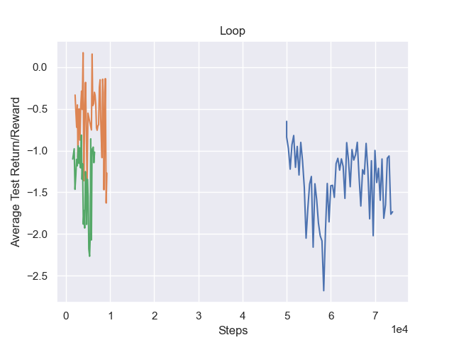
We compare the performance of DreamerV2 and our algorithm in three additional environments: Cartpole, SMARTS loop scenario, and SMARTS intersection 4lane scenario [1]. Further, we include the performance of our algorithm for both the case when an infinite Gaussian mixture is used in the VAE and when the single Gaussian mixture is used. Therefore, there are 3 algorithms in each plot.

References

[1] Zhou, M. and Luo, J. and Villella, J. and Yang, Y. and Rusu, D. and Miao, J. and Zhang, W. and Alban, M. and Fadakar, I. and Chen, Z. et al., SMARTS: Scalable Multi-Agent Reinforcement Learning Training School for Autonomous Driving, In Proceedings of the 4th Conference on Robot Learning (CoRL), 2020.
[2] Kingma, D. P. and Welling, M., Auto-encoding variational bayes, arXiv preprint arXiv:1312.6114, 2013.
[3] Kingma, D. P. and Ba, J., Adam: A method for stochastic optimization, arXiv preprint arXiv:1412.6980, 2014.
[4] Bosch, N. and Achterhold, J. and Leal-Taixe, L. and Stueckler, J., Planning from Images with Deep Latent Gaussian Process Dynamics, Proceedings of the 2nd Conference on Learning for Dynamics and Control, 120, 640–650, 2020.