Improving Cell-Free Massive MIMO Detection Performance via Expectation Propagation
Abstract
Cell-free (CF) massive multiple-input multiple-output (M-MIMO) technology plays a prominent role in the beyond fifth-generation (5G) networks. However, designing a high performance CF M-MIMO detector is a challenging task due to the presence of pilot contamination which appears when the number of pilot sequences is smaller than the number of users. This work proposes a CF M-MIMO detector referred to as CF expectation propagation (CF-EP) that incorporates the pilot contamination when calculating the posterior belief. The simulation results show that the proposed detector achieves significant improvements in terms of the bit-error rate and sum spectral efficiency performances as compared to the ones of the state-of-the-art CF detectors.
Index Terms:
Cell-free massive MIMO, distributed massive MIMO, expectation propagation, detection, pilot contamination.I Introduction
Cell-free (CF) massive multiple-input multiple-output (M-MIMO) technology has been proposed to deliver ubiquitous coverage and high service quality for beyond fifth-generation (5G) networks [1]. The access points (APs), known as the base station antennas in standard MIMO literature, are geographically distributed. The APs are managed by a central processing unit (CPU). Each user equipment (UE) is served simultaneously by all APs and therefore experiences no cell boundaries. This CF M-MIMO system provides additional diversity, increases the coverage probability, and mitigates the inter-cell interference, leading to a higher spectral efficiency (SE) and energy efficiency [2, 3, 4]. One of the critical issues is to design a detector for CF M-MIMO system which can overcome various impairments, in particular the pilot contamination, i.e. interference caused by pilot-sharing UEs [3].
The performance of the classical maximum ratio combining (MRC) detector in a CF M-MIMO system, referred to as CF-MRC detector, has been investigated in [2]. The CF-MRC detector estimates the transmitted symbols by multiplying corresponding received signals with the complex conjugate of the channel matrix. Although the CF-MRC detector can achieve an extremely low computational complexity, it fails to overcome the pilot contamination impact, which leads to a severe performance degradation [3]. To deal with the pilot contamination in CF M-MIMO systems, a modified minimum mean square error (MMSE) detector, referred to as CF-MMSE, has been proposed in [5]. It is shown to significantly outperform the CF-MRC detector by incorporating the statistical channel estimation error which contains the pilot contamination term when detecting the symbols. Specifically, the variance of the channel estimation error is incorporated into the regularization factor in case of the CF-MMSE detector. To further improve the performance of the CF-MMSE detectors, interference cancellation techniques have been combined with the CF-MMSE detectors as proposed in [4, 3, 6]. It is widely known that the MMSE with successive interference cancellation (SIC) detectors can achieve a high reliability performance at the cost of a higher computational complexity compared to the standard MMSE detector [7]. The CF-MMSE-SIC detector, combining the CF-MMSE scheme with the SIC scheme has been proposed in [3]. Unfortunately, the CF-MMSE-SIC detector provides only a minor performance gain compared to the CF-MMSE detector.
Recently, Bayesian machine learning techniques, called expectation propagation (EP) [8] and approximate message passing (AMP) [9], have been employed for detection to reduce the reliability performance gap between ML and suboptimal detectors in the collocated M-MIMO systems. In [9], the AMP algorithm has been shown to achieve a near optimal performance for independent and identically distributed (i.i.d.) Rayleigh fading channels. However, it performs poorly for non-i.i.d Rayleigh fading channels [10, 11]. The EP algorithm is an iterative algorithm used to infer estimates of the transmitted symbols by approximating their posterior probability density function (pdf) with factorizable Gaussian posterior belief [8]. For each posterior belief, EP retains only expectations such as mean and variance. The factorizable belief not only greatly reduces the complexity of the posterior pdf inference, but also enables the EP to achieve a near optimal performance [12].
We propose a novel iterative CF M-MIMO detector based on the EP algorithm, referred to as the CF-EP detector. The main contributions are summarized as follows:
- •
To the best of our knowledge, this is the first Bayesian detector for CF M-MIMO systems which can achieve a high detection reliability in the presence of the pilot contamination.
- •
The Gaussian posterior belief calculation of the original EP detector [8] is modified for systems with the pilot contamination, which is the main performance degradation factor in CF M-MIMO systems.
The simulation results demonstrate a significant BER and SE performance improvements compared to the state-of-the-art [2, 5, 4, 3] with a comparable computational complexity.
Notations: denotes an identity matrix. For any matrix , the notations , , , and stand for transpose, conjugate transpose, trace, and pseudo-inverse of , respectively. denotes the Frobenius norm of vector . denotes the complex conjugate of a complex number . is the mean of random vector , and is its variance. represents a complex single variate Gaussian distribution for a random variable with mean and variance . Let and .
II System Model
We consider an uplink CF M-MIMO system which consists of geographically distributed single-antenna APs, serving single antenna UEs, where . All APs send their pilot and data signals to the CPU which then estimates the channel state information (CSI) and transmitted symbols. We use a block fading model, where the channel between the -th UE and the -th AP is expressed as
| (1) |
Here, is the complex small scale fading coefficient and is the complex large-scale fading coefficient that describes geometric pathloss and shadowing. We assume that is known to the CPU. The channel is considered to be constant in time-frequency blocks of channel uses. Note that precise value of is unavailable to the receiver. Therefore, the channel is estimated by using the minimum mean-square error criterion, i.e. minimization of , where denotes the MMSE channel estimate of UE from AP . This results in an optimal estimation quality [13].
II-A Uplink Pilot Transmission and MMSE Channel Estimation
The channels between UEs and APs are estimated by using mutually orthogonal pilot signals with and . The pilots are randomly assigned to the UEs. In practice, which results in a pilot contamination [2]. Let be the index of the pilot signal assigned to the -th UE, . Obviously, . We group UEs into sets such that all UEs in the set use the same pilot, i.e. for . At AP , the received pilot is given as follows,
| (2) |
where is the uplink transmit power of a UE11 1 All UEs are assumed to transmit with equal power. and is an additive Gaussian noise with zero mean and variance equal to the noise power.
The MMSE channel estimate of UE from AP is given in [3] as
| (3) |
By substituting in (2) into (3), we obtain
| (4) |
where each element in follows a Gaussian distribution with zero mean and variance . From (4) and (1), we can easily verify that and , . Therefore, the channel estimation error of UE from AP
| (5) |
follows a Gaussian distribution with mean zero and variance . The channel estimation error from the -th UE to all APs is defined in a vector form as , where . The covariance matrix is an diagonal matrix whose diagonal elements are . The channel estimation error matrix for UEs, can be written as
| (6) |
Since , the channel estimation error matrix is normally distributed with zero mean and covariance matrix , i.e. .
II-B Uplink Data Transmission
All UEs map their information bit streams to symbols that belong to constellation of -QAM, , where . The -th user symbol is denoted as . The average symbol energy is . The channel matrix between UEs and APs and its estimate are denoted as and , respectively. The -th elements of and are defined by (1) and (3), respectively. The received signal of all APs, , available at the CPU, is given as
| (7) |
where is a Gaussian noise and is uniformly distributed on . By substituting in (6) into (7), we obtain
| (8) |
at the CPU. To detect the symbols we can use the MMSE channel estimate , which introduces the channel estimation error as explained in the Section IIA. Considering that and , we define a new noise vector .
III Cell-Free Expectation Propagation Detector
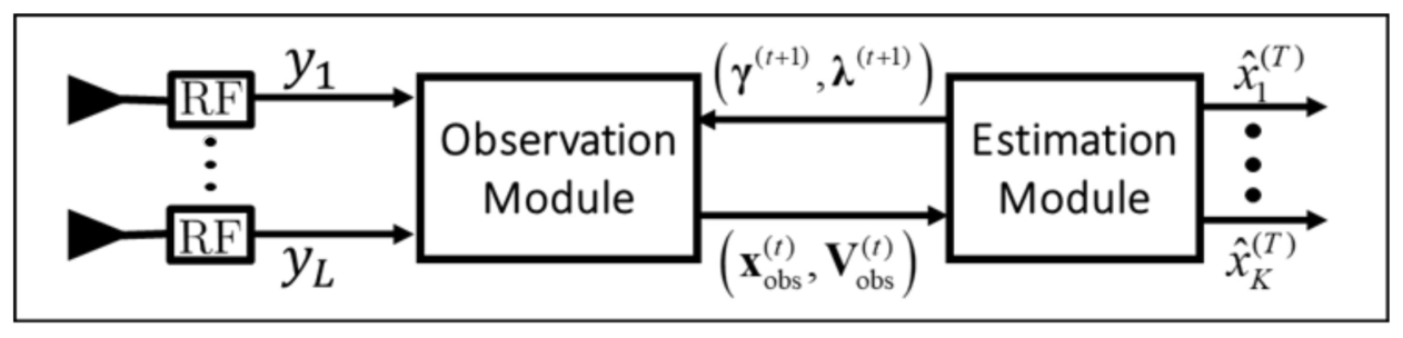
In this section, we propose a novel CF M-MIMO detector based on the EP concept [8]. Our detector takes the effect of the pilot contamination into consideration. We refer it as the cell-free expectation propagation (CF-EP) detector with the architecture shown in Fig. 1. The CF-EP consists of two modules: the observation module calculating the posterior beliefs based on the received signal and the estimation module yielding soft transmitted symbol estimates. The CF-EP iteratively exchanges the outputs of both modules until the convergence criterion is satisfied.
III-A The Observation Module
Given the received signal in (8), the posterior distribution of the transmitted symbols is characterized by
| (9) |
where is a priori pdf of , is the Dirac delta function, and is omitted as it does not depend on the distribution of . A direct calculation of (9) results in a prohibitively intensive computation as we need to consider all possible combinations of the symbols. Therefore, EP is used to iteratively construct a Gaussian approximation to the true posterior distribution of the transmitted symbol vector.
Concretely, the EP constructs a Gaussian posterior belief , where is the iteration number. This involves replacing in (9) with a distribution from the exponential family, [14]. Here, is a diagonal matrix with diagonal elements and . Both and are complex numbers with and . To calculate the Gaussian posterior belief, we first treat as a random vector and approximate as . Note that the matrix corresponds to the channel estimation error variance which is caused by the pilot contamination, defined in Section IIA. The Gaussian posterior belief is then expressed as
| (10) |
We can compute the product of two Gaussians in (III-A) by using the Gaussian product property22 2 The product of two Gaussians results in another Gaussian, ., given in Appendix A.1 of [15]. By using this property, we obtain the variance and mean of as
| (11a) | ||||
| (11b) | ||||
Remark 1 (CF-EP Gaussian posterior belief)
We then compute based on ,
| (12) |
where and is a diagonal matrix with as the -th diagonal element, which can be expressed as
| (13a) | ||||
| (13b) | ||||
Here, is the -th element of vector and is the -th diagonal element of matrix . The pair from (11) is then forwarded to the estimation module.
III-B The Estimation Module
Based on provided by the observation module, the estimation module computes a new posterior belief
| (14) |
This is different from the Gaussian posterior belief in (III-A), obtained based on from exponential families. In fact, the EP algorithm is used to ensure a similarity between the mean-variance pairs of and . This similarity is specified in [16] by the moment matching (MM) condition, minimizing the Kullback-Leibler divergence between posterior beliefs. The MM condition is expressed as follows
| (15) |
where denotes the first two moments, i.e. the mean and variance of with respect to . Furthermore, the mean and variance of are given in [8] as
| (16a) | |||
| (16b) |
Here, is the normalization constant to ensure that . The iteration of the CF-EP detector will be terminated when
| (17) |
i.e. when (15) is satisfied, or once the algorithm once the maximum number of iterations is reached. Hard estimates of the transmitted symbols are then made from , by comparing its Euclidean distance from the transmitted -QAM symbol sets where is the last iteration number.
Until (15) is satisfied, the estimation module will re-evaluate the Gaussian posterior belief, , by first calculating based on the , expressed as
| (18) |
where
| (19a) | ||||
| (19b) | ||||
Note that and are referred to as the updating parameters as they are used to update the Gaussian posterior beliefs. We smoothen the update of by using a convex combination with the former values,
| (20a) | ||||
| (20b) | ||||
where is a weighting coefficient.
The estimation module sends the updating parameters to the observation module, as illustrated in Fig. 1. The complete pseudo-code is shown in Alg. 1. One can also compute the SE of the CF-EP detector by using signal-to-interference-noise ratio, given in[17] as
| (21) |
where .
IV Numerical Results
We follow the simulation setup used in [3]. Specifically, we consider single-antenna APs, randomly deployed in a km area, serving randomly located UEs, in an urban environment complying with 3GPP Urband Microcell model [18]. The large scale fading coefficient is given as
| (22) |
where is the distance between AP and UE and is the shadow fading. The shadowing terms from an AP to different UEs are correlated as , where is the distance between UE and UE . The pilots are randomly indexed and assigned to all UEs. We employ -QAM modulation scheme and set the signal-to-noise ratio (SNR) dB. We evaluate the performance depending on the pilot-to-user ratio defined as . Finally, we compare the performance of our proposed detector with the CF-MRC [2], CF-MMSE [5], and CF-MMSE-SIC [3] detectors.
IV-A Convergence and Complexity Analyses
We first analyse the convergence behaviour of the proposed CF-EP detector by plotting the average number of iterations needed to satisfy the MM condition in (15). It can be seen from Fig. 2 that the CF-EP detector needs less than iterations to converge for various pilot-to-user ratios, .
As tabulated in Table 1, the computational complexity of the CF-EP detector is slightly higher than the MMSE detector depending on its number of iterations. The CF-EP requires on average iterations to converge. Therefore, the complexity order of the CF-EP detector remains the same as the CF-MMSE detector. Note that the detector will be implemented at the CPU, which is assumed to be equipped with a high performance computer. Therefore, a minor increase in the computational complexity will not be a critical issue.
| Detector | Complexity |
|---|---|
| CF-MRC | |
| CF-MMSE | |
| CF-MMSE-SIC | |
| CF-EP |
IV-B Performance Analysis
To analyse the proposed detector’s performance, we plot the BER and sum SE over the random users locations versus the pilot-to-user ratio. Fig. 3a demonstrates that the CF-EP detector outperforms the CF-MMSE-SIC and the CF-MMSE detectors in terms of BER, for all pilot-to-user-ratio . More specifically, the CF-EP detector can achieve BER with around lower pilot-to-user ratio than the CF-MMSE and CF-MMSE-SIC detectors. In Fig. 3b, the CF-EP detector demonstrates and sum SE improvements compared to the CF-MMSE and CF-MMSE-SIC detectors, respectively. From these facts, we conclude that the developed EP based detector, dealing with the pilot contamination impact, achieves a significant performance gain compared to the existing CF M-MIMO detectors.
V Conclusion
We propose a novel EP based detector for CF M-MIMO systems, namely the CF-EP detector. Our simulation results show that the BER and sum SE performances of the CF-EP detector are better than those of the state-of-the-art CF M-MIMO detectors with comparable computational complexity.
Acknowledgment
This research was supported by the research training program stipend from The University of Sydney. The work of Branka Vucetic was supported in part by the Australian Research Council Laureate Fellowship grant number FL160100032.
References
- [1] J. Zhang, E. Björnson, M. Matthaiou, D. W. K. Ng, H. Yang and D. J. Love, “Prospective multiple antenna technologies for beyond 5G,” IEEE J. Sel. Areas Commun., vol. 38, no. 8, pp. 1637–1660, Aug. 2020.
- [2] H. Q. Ngo, A. Ashikhmin, H. Yang, E. G. Larsson, and T. L. Marzetta, “Cell-free massive MIMO versus small cells,” IEEE Trans. Wireless Commun, vol. 16, no. 3, pp. 1834–1850, Mar. 2017.
- [3] E. Björnson and L. Sanguinetti, “Making cell-free massive MIMO competitive with MMSE processing and centralized implementation,” IEEE Trans. Wireless Commun, vol. 19, no. 1, pp. 77–90, Jan. 2020.
- [4] Y. Feng, M. Wang, D. Wang, and X. You, “Low complexity iterative detection for a large-scale distributed MIMO prototyping system,” in Proc. IEEE Int. Conf. on Commun., China, May. 2019, pp. 1–6.
- [5] E. Nayebi, A. Ashikhmin, T. L. Marzetta and B. D. Rao, “Performance of cell-free massive MIMO systems with MMSE and LSFD receivers,” in Proc. 50th Asilomar Conf. on Signals, Syst. and Comput., USA, Nov. 2016, pp. 203–207.
- [6] R. Mosayebi, M. M. Mojahedian and A. Lozano, “Linear interference cancellation for the cell-free C-RAN uplink,” IEEE Trans. Wireless Commun, Nov. 2020.
- [7] T. Liu and Y. Y. Liu, “Modified fast recursive algorithm for efficient MMSE-SIC detection of the V-BLAST system,” IEEE Trans. Wireless Commun, vol. 7, no. 10, pp. 3713–3717, Oct. 2008.
- [8] J. Céspedes, P. M. Olmos, M. Sánchez-Fernández, and F. Pérez-Cruz, “Expectation propagation detection for high-order high-dimensional MIMO systems,” IEEE Trans. Commun., vol. 62, no. 8, pp. 2840–2849, Aug. 2014.
- [9] M. Bayati and A. Montanari, “The dynamics of message passing on dense graphs with applications to compressed sensing,” IEEE Trans. Inf. Theory, vol. 57, no. 2, p. 764–785, Feb. 2011.
- [10] S. Rangan, P. Schniter and A. K. Fletcher, “Vector approximate message passing,” in IEEE Int. Symp. on Inform. Theory (ISIT), Germany, June 2017, pp. 1588–1592.
- [11] K. Takeuchi and C. Wen, “Rigorous dynamics of expectation-propagation signal detection via the conjugate gradient method,” in IEEE 18th Int. Workshop on Sig. Process. Adv. in Wireless Commun. (SPAWC), Japan, June 2017, pp. 1–5.
- [12] A. Kosasih, W. Hardjawana, B. Vucetic, and C. K. Wen, “A linear Bayesian learning receiver scheme for massive MIMO systems,” in Proc.IEEE Wireless Commun. and Netw. Conf., Korea, May. 2020, pp. 1–6.
- [13] E. Björnson, J. Hoydis, and L. Sanguinetti, “Massive MIMO networks: Spectral, energy, and hardware efficiency,” Found. Trends Mach. Learn., vol. 11, no. 3-4, pp. 154–655, 2017.
- [14] J. Zhang, Y. He, Y. W. Li, C. K. Wen, and S. Jin, “Meta learning-based MIMO detectors: Design, simulation, and experimental test,” IEEE Trans. Wireless Commun., Oct. 2020.
- [15] C. E. Rasmussen and C. K. I. Williams, Gaussian processes for machine learning. MIT Press, 2006.
- [16] T. P. Minka, “Expectation propagation for approximate bayesian inference,” in Proc. of the 17th conf. on Uncertainty in artificial intell., 2001, pp. 362–369.
- [17] E. Biglieri, J. Proakis, and S. Shamai, “Fading channels: Information theoretic and communications aspects,” IEEE Trans. Inf. Theory, vol. 44, no. 6, pp. 2619–2691, Oct. 1998.
- [18] 3rd Generation Partnership Project (3GPP), “Further advancements for E-UTRA physical layer aspects (Release 9),” 3GPP TS 36.814, Tech. Rep., Mar. 2017.