Endure: A Robust Tuning Paradigm for LSM Trees Under Workload Uncertainty
Abstract.
Log-Structured Merge trees (LSM trees) are increasingly used as the storage engines behind several data systems, frequently deployed in the cloud. Similar to other database architectures, LSM trees take into account information about the expected workload (e.g., reads vs. writes, point vs. range queries) to optimize their performance via tuning. Operating in shared infrastructure like the cloud, however, comes with a degree of workload uncertainty due to multi-tenancy and the fast-evolving nature of modern applications. Systems with static tuning discount the variability of such hybrid workloads and hence provide an inconsistent and overall suboptimal performance.
To address this problem, we introduce Endure – a new paradigm for tuning LSM trees in the presence of workload uncertainty. Specifically, we focus on the impact of the choice of compaction policies, size-ratio, and memory allocation on the overall performance. Endure considers a robust formulation of the throughput maximization problem, and recommends a tuning that maximizes the worst-case throughput over a neighborhood of each expected workload. Additionally, an uncertainty tuning parameter controls the size of this neighborhood, thereby allowing the output tunings to be conservative or optimistic. Through both model-based and extensive experimental evaluation of Endure in the state-of-the-art LSM-based storage engine, RocksDB, we show that the robust tuning methodology consistently outperforms classical tuning strategies. We benchmark Endure using 15 workload templates that generate more than 10000 unique noisy workloads. The robust tunings output by Endure lead up to a 5 improvement in throughput in presence of uncertainty. On the flip side, when the observed workload exactly matches the expected one, Endure tunings have negligible performance loss.
Proceedings of the VLDB Endowment, Vol. 15, No. 1 ISSN 2150-8097.
doi:XX.XX/XXX.XX
PVLDB Artifact Availability:
The source code, data, and/or other artifacts have been made available at https://github.com/BU-DiSC/endure.
1. Introduction
Ubiquitous LSM-based Key-Value Stores. Log-Structured Merge trees (LSM trees) is the most commonly deployed data structure used in the backend storage of modern key-value stores (O’Neil et al. 1996). LSM trees offer high ingestion rate and fast reads, making them widely adopted by systems such as RocksDB (Facebook 2021) at Facebook, LevelDB (Google 2021) and BigTable (Chang et al. 2006) at Google, HBase (HBase 2013), Cassandra (Apache 2021) at Apache, WiredTiger (WiredTiger 2021) at MongoDB, X-Engine (Huang et al. 2019) at Alibaba, and DynamoDB (DeCandia et al. 2007) at Amazon.
LSM trees store incoming data in a memory buffer, which is flushed to storage when it is full and merged with earlier flushed buffers to form a collection of sorted runs with exponentially increasing sizes (Luo and Carey 2020). Frequent merging of sorted runs leads to higher merging costs but facilitates faster lookups (leveling). On the flip side, lazy merging policies (tiering) trade lookup performance for lower merging costs (Sarkar et al. 2021). Maintaining a separate Bloom filter (Bloom 1970) per sorted run optimizes point queries by avoiding unnecessary accesses to runs that do not contain the desired data. Range query performance does not benefit from the presence of Bloom filters, yet, it depends on the LSM tree structure.
Tuning LSM trees. As the number of applications relying on LSM-based storage backends increases, the problem of performance tuning for LSM trees has garnered a lot of attention. A common assumption made by all these methods is that one has complete knowledge about the expected workload and the execution environment. Given such knowledge, prior work optimizes for the memory allocation to Bloom filters across different levels, memory distribution between the buffers and the Bloom filters, and the choice of merging policies (i.e., leveling or tiering) (Dayan et al. 2017; Dayan et al. 2018). Different optimization objectives have led to hybrid merging policies with more fine-grained tunings (Dayan and Idreos 2018; Dayan and Idreos 2019; Idreos et al. 2019), optimized memory allocation strategies (Bortnikov et al. 2018; Kim et al. 2020; Luo 2020), variations of Bloom filters (Luo et al. 2020; Zhang et al. 2018; Zhang et al. 2020a), new compaction routines (Alkowaileet et al. 2020; Luo and Carey 2019; Sarkar et al. 2020; Sarkar et al. 2021; Zhang et al. 2020b), and exploitation of data characteristics (Yang et al. 2020; Ren et al. 2017; Absalyamov et al. 2018).
The Only Certainty is Uncertainty. Even when accurate information about the workload and underlying hardware is available, tuning data systems is a notoriously difficult research problem (Chaudhuri et al. 2004; Chaudhuri and Weikum 2005; Shasha and Bonnet 2002). The explosive growth in the public and private use of the cloud infrastructure for data management (Hayes 2008; Intel 2011; Research 2019) has exacerbated this problem because of increased uncertainty and variability in workloads (Chohan et al. 2010; Galante and Bona 2012; Herbst et al. 2013; Holze et al. 2010; Mohan 2016; Özcan et al. 2017; Pezzini et al. 2014; Schnaitter et al. 2006; Schnaitter et al. 2007; Schnaitter and Polyzotis 2012; Wolski et al. 2017).
An Example. Before describing our framework, we give an example that depicts how variation in observed workloads relative to the expected workload – used during tuning of the LSM tree-based storage – leads to suboptimal performance. In Figure 1, the -axis shows a sequence of workloads executed over an LSM-based engine, while the -axis shows the average disk accesses per workload. The experiment is split into three sessions – the first and the last sessions receive the expected workload, while the second session receives a different workload. Although it has the same reads vs. writes ratio as the expected workload, it has a higher percentage of short range queries in comparison to the point queries. The solid black line shows the performance of a system tuned for the expected workload. Note that the average I/Os increase dramatically in the second session even though the amount of data being read is approximately the same. On the other hand, the blue line corresponds to each session having its ideal tuning, leading to only half as many I/Os per operation. Note that it is not feasible to continually change tunings during execution, as it requires redistribution of the allocated memory between different components of the tree and potentially changing its shape. Hence, we want to find a tuning that is close-to-optimal for both the expected and the observed workload.
Our Work: Robust LSM Tree Tuning. To address this suboptimality caused by variations in the observed workload, we depart from the classical view of database tunings which assumes accurate knowledge about the expected workload. Rather, we introduce Endure, a new robust tuning paradigm that incorporates expected uncertainty into optimization and apply it to LSM trees.
We propose a problem formulation that seeks an LSM tree configuration that maximizes the worst-case throughput over all the workloads in the neighborhood of an expected workload and call it the Robust Tuning problem. We use the notion of KL-divergence between probability distributions to define the neighborhood size, implicitly assuming that the uncertain workloads would be contained in the neighborhood. As the KL-divergence boundary condition approaches zero, our problem becomes equivalent to the classical optimization problem (referred henceforth as the Nominal Tuning problem). More specifically, our approach uses as input the expected size of the uncertainty neighborhood, which dictates the qualitative characteristics of the solution. Intuitively, the larger the size of the uncertainty region, the larger the workload discrepancy a robust tuning can absorb. Leveraging work on robust optimization from the Operations Research community (Bertsimas et al. 2010a; Ben-Tal and Nemirovski 1998; Ben-Tal et al. 2013b), we efficiently solve the Robust Tuning problem and find the robust tuning for LSM tree-based storage systems. A similar problem of using workload uncertainty while determining the physical design of column-stores has been explored in prior work (Mozafari et al. 2015). However, their methodology is not well suited for the LSM tuning problem. We provide additional details regarding this in Section 9.
Contributions. To the best of our knowledge, our work presents the first systematic approach for robust tuning of LSM tree-based key-value stores under workload uncertainty. Our technical and practical contributions can be summarized as follows:
- •
- •
We augment existing analytical cost models of LSM tree-based storage engines with more precise estimates of workload execution costs (§5).
- •
In our model-based analysis, we show that robust tunings from Endure provide up to 5 higher throughput when faced with uncertain workloads, and match classical tuning performance when there is no uncertainty (§7).
- •
We integrate Endure into RocksDB, a state-of-the-art LSM storage engine, where we show both system I/O and latency reductions of up to . Additionally, we show that Endure scales with database size (§8).
- •
To encourage reproducible research, we make our robust tuning framework publicly available (Andy Huynh, Harshal A. Chaudhari, Evimaria Terzi, and Manos Athanassoulis 2021).

2. Background on LSM Trees
Basics. LSM trees use the out-of-place ingestion paradigm to store key-value pairs. Writes, updates, or deletes are buffered in a memory buffer, and once full, its contents are sorted based on the key, forming an immutable sorted run. This run is then flushed to the first level on secondary storage. Each level of sorted runs has a tunable maximum permitted size. Overall, for an LSM tree with disk-resident levels, we denote the memory buffer as Level , and the remaining levels in storage to . The disk-resident sorted runs have exponentially increasing sizes following a tunable size ratio . Figure 2 shows an overview of an LSM tree.
We denote the number of bits of main memory allocated to the buffer as , which holds a number of entries with fixed entry size . For example, in RocksDB the default buffer size is MB, and depending on the application, the entry size typically varies between 64B and 1KB.
Level 0 can be updated in-place as it is in memory, however, runs in levels 1 and beyond are immutable. Each level has a capacity threshold of entries, thus, level capacities are exponentially increasing by a factor of . The total number of levels for a given is
| (1) |
where is the total number of entries across all levels (Dayan et al. 2018; Luo et al. 2020; Sarkar et al. 2020).
Compaction Policies: Leveling and Tiering. Classically, LSM trees support two merging policies: leveling and tiering. In leveling, each level may have at most one run, and every time a run in Level () is moved to Level , it is greedily sort-merged (compaction) with the run from Level , if it exists. With tiering, every level must accumulate runs before they trigger a compaction. During a compaction, entries with a matching key are consolidated and only the most recent valid entry is retained (Dong et al. 2017; O’Neil et al. 1996). Recently hybrid compaction policies fuse leveling and tiering in a single tree to strike a balance between the read and write throughput (Dayan and Idreos 2018; Dayan and Idreos 2019).
LSM tree Operations. An LSM tree supports: (a) writes of new key-value pairs, (b) point queries, and (c) range queries.
Writes: A write operation is handled by a buffer append, and if the buffer gets full, it triggers a compaction. Any write may include either a new key-value pair, an existing key that updates its value, or a special entry that deletes an existing key.
Point Queries: A point query searches for the value of a specific unique key. It begins by looking at the memory buffer, then traverses the tree from the smallest to the largest level. For tiering, within a level, a lookup moves from the most to the least recent tier. The lookup terminates when it finds the first matching entry. Note that a point query might return an empty or a non-empty result. We differentiate the two because, in general, workloads with empty point queries can be further optimized (Dayan et al. 2017; Dayan et al. 2018).
Range Queries: A range lookup returns the most recent versions of the target keys by sort-merging all qualifying runs from the tree.
Optimizing Lookups. Read performance is optimized using Bloom filters and fence pointers. In the worst case, a lookup needs to probe every run. To reduce this cost, LSM engines use one Bloom filter per run in main memory (Dayan et al. 2017; Facebook 2021). Bloom filters (Bloom 1970) are probabilistic membership test data structures that exhibit a false positive as a function of the ratio between the memory allocated to them and the elements it indexes. In LSM trees, Bloom filters allow a lookup to skip probing a run altogether if the filter-lookup returns negative. In practice, for efficient storage, Bloom filters are maintained at the granularity of files (Dong et al. 2017). Fence pointers store the smallest key per disk page in memory (Dayan et al. 2017), to quickly identify which page(s) to read for a lookup, and perform up to one I/O per run for point lookups.
Tuning LSM Trees. Prior to this work, efforts to systematically tune LSM trees assume that the workload information and the execution environment are accurately known. Under that assumption, the main focus on LSM tuning has been on deciding how to allocate the available main memory between Bloom filters and buffering (Dayan et al. 2017; Kim et al. 2020; Luo 2020), while often the size ratio and the merging strategy was also co-tuned (Dayan et al. 2018). Such design decisions are common across industry standard LSM-based engines such as Apache Cassandra (Apache 2021), AsterixDB (Alsubaiee et al. 2014), RocksDB (RocksDB 2020b), and InfluxDB (influxdata [n. d.]). In addition, recent work has introduced new hybrid merging strategies (Dayan and Idreos 2018; Dayan and Idreos 2019; Sarkar et al. 2021), and optimizations for faster data ingestion (Luo et al. 2019) and performance stability (Luo and Carey 2019).
3. Problem Definitions
In this section, we provide the formal problem definitions on how to choose the design parameters of an LSM tree. Before proceeding, we give a brief introduction to our notation.
3.1. Notation
As we discussed above, LSM trees have two types of parameters: the design parameters that are changed primarly for performance, and the system parameters that are given and therefore untunable.
Design Parameters. The design parameters we consider in this paper are the size-ratio (), the memory allocated to the Bloom filters (), the memory allocated to the write buffer () and the compaction policy (). These are ubiquitous design parameters and have been extensively studied as having the largest impact on performance (Dayan et al. 2017; Dayan et al. 2018; Luo and Carey 2020). Therefore, we focus on these parameters in order to define a problem that is agnostic to the LSM engine used. Recall that the policy refers to either leveling or tiering, as discussed in the previous section.
System Parameters. A complex data structure like an LSM tree also has various system parameters and other non-tunable ones (e.g., total memory (), data entry size , page size , data size ).
LSM Tree Configuration. For notation, we use to denote the LSM tree tuning configuration which describes the values of the tunable parameters together . Note that we only use the memory for Bloom filters and not , because the latter can be derived using the former and total available memory: .
Workload. The choice of the parameters in depends on the input (expected) workload, i.e., the fraction of empty lookups (), non-empty lookups (), range lookups (), and write () queries. Note that this workload representation is common for analyzing and tuning LSM trees (Dayan et al. 2018; Luo and Carey 2020). Additionally, complex workloads (i.e., SQL statements) generate access patterns on the storage engine and can be broken down into the same basic operations. This mapping of complex queries to basic operations is also common for performance tuning of LSM tree-based storage engines (Cao et al. 2020). Therefore a workload can be expressed as a vector describing the proportions of the different kinds of queries. Clearly, or alternatively: where denotes a column vector of ones.
| Type | Term | Definition |
|---|---|---|
| Design | Memory allocated for Bloom filters | |
| Memory allocated for the write buffer | ||
| Size ratio between consecutive levels | ||
| Compaction policy (tiering/leveling) | ||
| System | Total memory (filters+buffer) () | |
| Size of a key-value entry | ||
| Number of entries that fit in a page | ||
| Total number of entries | ||
| Workload | Percentage of zero-result point lookups | |
| Percentage of non-zero-result point lookups | ||
| Percentage of range queries | ||
| Percentage of writes |
Each type of query (non-empty lookups, empty lookups, range lookups and writes) has a different cost, denoted as , , , , as there is a dependency between the cost of each type of query and the design . For ease of notation, we use to denote the vector of the costs of executing different types of queries. Thus, given a specific configuration () and a workload (), the expected cost for the workload can be computed as:
| (2) |
We present a summary of all of our notation in Table 1.
3.2. The Nominal Tuning Problem
Traditionally, the designers have focused on finding the configuration that minimizes the total cost , for a given fixed workload . We call this problem the Nominal Tuning problem, defined as follows:
Problem 1 (Nominal Tuning).
Given fixed find the tuning configuration of the LSM tree such that
| (3) |
The nominal tuning problem described above captures the classical tuning paradigm. It uses a cost-model to find a system configuration that minimizes the cost given a specific workload and system environment. Specifically, prior tuning approaches for LSM trees solve the nominal tuning problem when proposing optimal memory allocation, and merging policies (Dayan et al. 2017; Dayan et al. 2018; Luo 2020).
3.3. The Robust Tuning Problem
In this work, we attempt to compute high-performance configurations that minimize the expected cost of operation, as expressed in Equation (2), in the presence of uncertainty with respect to the expected workload.
The Nominal Tuning problem assumes perfect information about the workload for which to tune the system. For example, we may assume that the input vector represents the workload for which we optimize, while in practice, is simply an estimate of what the workload will look like. Hence, the configuration obtained by solving Problem 1 may result in high variability in the system performance that will inevitably depend on the actual observed workload upon the deployment of the system.
We capture this uncertainty by reformulating Problem 1 to take into account the variability that can be observed in the input workload. Given an expected workload , we introduce the notion of the uncertainty region of , which we denote by .
We can define the robust version of Problem 1, under the assumption that there is uncertainty in the input workload as follows:
Problem 2 (Robust Tuning).
Given and uncertainty region find the tuning configuration of the LSM tree such that
| (4) | s.t., |
Note that the above problem definition intuitively states the following: it recognizes that the input workload won’t be observed exactly, and it assumes that any workload in is possible. Then, it searches for the configuration that is best for the worst-case scenario among all those in .
The challenge in solving Robust Tuning is that one needs to explore all the workloads in the uncertainty region in order to solve the problem. In the next section, we show that this is not necessary. In fact, by appropriately rewriting the problem definition we show that we can solve Problem 2 in polynomial time.
4. Algorithms for ROBUST TUNING
In this section, we discuss our solutions to the Robust Tuning problem. On a high level, the solution strategy is the following: first, we express the objective of the problem (as expressed in Equation (2)) as a standard continuous optimization problem. We then take the dual of this problem and use existing results in robust optimization to show: the duality gap between the primal and the dual is zero, and the dual problem is solvable in polynomial time. Thus, the dual solution can be translated into the optimal solution for the primal, i.e., the original Robust Tuning problem. The specifics of the methodology are described below:
Defining the Uncertainty Region . Recall that is a probability vector, i.e., . Thus, in order to define the uncertainty region , we use the Kullback-Leibler (KL) divergence function (Kullback et al. 1951). KL-divergence for two probability distributions is defined as follows:
Definition 0.
The KL-divergence distance between two vectors and in is defined as,
Note that we could have potentially used other divergence functions (Pardo 2018) instead of the KL-divergence. We use the KL-divergence as we believe it fits our goal and intuitive understanding of the space of workloads.
Using the notion of KL-divergence we can now formalize the uncertainty region around an expected workload as follows,
| (5) |
Here, determines the maximum KL-divergence that is allowed between any workload in the uncertainty region and the input expected workload . Note that the definition of the uncertainty region takes as input the parameter , which intuitively defines the neighborhood around the expected workload. This can be computed as the mean KL-divergence from the historical workloads.
In terms of notation, input is required for defining the uncertainty region . However, we drop the superscript notation unless required for context.
Rewriting of the ROBUST TUNING Problem (Primal). Using the above definition of the workload uncertainty region , we are now ready to proceed to the solution of the Robust Tuning problem. For a given , the problem definition as captured by Equation (2) can be rewritten as follows:
| (6) |
Note that the above equation is a simple rewrite of Equation (6) that captures the intuition that the optimization is done over the worst-case workload among all the workloads in the uncertainty region . An equivalent way of writing Equation (6) is by introducing an additional variable , then writing the following:
| (7) | s.t., |
This reformulation allows us to remove the term in the objective from Equation (6). The constraint in Equation (4) can be equivalently expressed as,
Finally, the Lagrange function for the optimization on the right-hand side of the above equation is:
where and are the Lagrangian variables.
Formulating the Dual Problem. We can now express the dual objective as,
| (8) |
which we need to minimize.
Now we borrow the following result from (Ben-Tal et al. 2013a),
Lemma 4.2 ((Ben-Tal et al. 2013a)).
A configuration is the optimal solution to the Robust Tuning problem if and only if where the minimum is attained for some value of .
In other words, minimizing the dual objective (as expressed in Equation (8)) will lead to the optimal solution for the Robust Tuning problem.
Solving the Dual Optimization Problem Optimally. Formulating the dual problem and using the results of Ben-Tal et al. (Ben-Tal et al. 2013a), we have shown that the dual solution leads to the optimal solution for the Robust Tuning problem. Moreover, we can obtain the optimal solution to the original Robust Tuning problem in polynomial time, a consequence of the tractability of the dual objective.
To solve the dual problem, we first simplify the dual objective so that it takes the following form:
| (9) |
In Equation (9), denotes the conjugate of KL-divergence function and corresponds to the -th dimension of the cost vector as defined in Section 3.1 – clearly in this case as we have types of queries in our workload. Results of Ben-Tal et al. (Ben-Tal et al. 2013a) show that minimizing the dual function as described in Equation (9) is a convex optimization problem, and it can be solved optimally in polynomial time if and only if the cost function is convex in all its dimensions.
In our case, the cost function for the range queries is not convex w.r.t. size-ratio for the tiering policy. However, on account of its smooth non-decreasing form, we are still able to find the global minimum solution for
| (10) |
This minimization problem can be solved using the Sequential Least Squares Quadratic Programming solver (SLSQP) included in the popular Python optimization library SciPy (Virtanen et al. 2020). Solving this problem outputs the values of the Lagrangian variables and and most importantly the configuration that optimizes the objective of the Robust Tuning problem – for input . In terms of running time, SLSQP solver outputs a robust tuning configuration for a given input in less than a second.
5. The Cost Model of LSM Trees
In this section, we provide the detailed cost model used in Endure to accurately capture the behavior of an LSM tree. Following prior work on LSM trees (Dayan et al. 2018; Luo et al. 2020), we focus on four types of operations: point queries that return an empty result, point queries that have a match, range queries, and writes.
5.1. Model Basics
When modeling the read cost of LSM trees, a key quantity to accurately capture is the amount of extra read I/Os that take place. While Bloom filters are used to minimize those, they allow a small fraction of false positives. In particular, a point lookup probes a run’s filter before accessing the run in secondary storage. If the filter returns negative, the target key does not exist in the run, and so the lookup skips accessing the run and saves one I/O. If a filter returns positive, then the target key may exist in the run, so the lookup probes the run at a cost of one I/O. If the run actually contains the key, the lookup terminates. Otherwise, we have a false positive and the lookup continues to probe the next run. False positives increase the I/O cost of lookups. The false positive rate () of a standard Bloom filter designed to query entries using a bit-array of size is shown by (Tarkoma et al. 2012) to be calculated as follows:
Note that the above equation assumes the use of an optimal number of hash functions in the Bloom filter (Wikipedia contributors 2021).
Classically, LSM tree based key-value stores use the same number of bits-per-entry across all Bloom filters. This means that a lookup probes on average of the runs, where is the overall amount of main memory allocated to the filters. As approaches 0 or infinity, the term approaches 1 or 0 respectively. Here, we build on of the state-of-the-art Bloom filter allocation strategy proposed in Monkey (Dayan et al. 2017; Dayan et al. 2018) that uses different false positive rates at different levels of the LSM tree to offer optimal memory allocation; for a size ratio , the false positive rate corresponding to the Bloom filter at the level is given by
| (11) |
Additionally, false positive rates for all levels satisfy . It should be further noted that Monkey optimizes false positive rates at individual levels to minimize the worst case average cost of empty point queries. Non-empty point query costs, being significantly lower than those of empty point queries, are not considered during the optimization process.
LSM Tree Design & System Parameters. In Section 3.1 we introduced the key design and system parameters needed to model LSM tree performance. In addition to those parameters, there are two auxiliary and derived parameters we use in the cost model presented in this section: the potential storage asymmetry in reads and writes () and the expected selectivity of range queries ().
5.2. The Cost Model
In this section, we model the costs in terms of expected number of I/O operations required for the fulfillment of the individual queries.
Expected Empty Point Query Cost (). A point query that returns an empty result will have to visit all levels (and every sorted run of every level for tiering) where false positives in the Bloom filters trigger I/O operations. Thus, the expected number of I/O operations per level depends on the Bloom filter memory allocation at that level. Hence, Equation (12) expresses in terms of the false positive rates at each level:
| (12) |
In the leveling policy, each level has exactly one run. On the other hand, with tiering policy, each level has up to runs. All runs at the same level in tiering have equal false positives rates on account of their equal sizes.
Expected Non-empty Point Query Cost (). There are two components to the expected non-empty point query cost. First, we assume that the probability of a point query finding a non-empty result in a level is proportional to the size of the level. Thus, the probability of such a query being satisfied on level by a unit cost I/O operation is simply , where denotes the number of entries in a tree completely full upto levels. Thus,
| (13) |
Second, we assume that all levels preceding level trigger I/O operations with probability equivalent to the false positive rates of the Bloom filters at those levels. Similar to the empty point queries, the expected cost of such failed I/Os on preceding levels is simply . In the case of tiering, we assume that on average, the entry is found in the middle run of the level resulting in an additional extra I/O operations. Thus, we can compute the non-empty point query cost as an expectation over the entry being found on any of the levels of the tree as follows:
| (14) |
Range Queries Cost (). A range query issues or disk seeks (one per run) for leveling and tiering respectively. Each seek is followed by a sequential scan. The cumulative number of pages scanned over all runs is , where is the average proportion of all entries included in range lookups. Hence, the overall range lookup cost in terms of pages reads is as follows:
| (15) |
Write Cost (). We model worst-case writing cost assuming that the vast majority of incoming entries do not overlap. This means that most entries will have to propagate through all levels of the LSM tree. Following the state-of-the-art write cost model, we assume that every written item participated in and merges with tiering and leveling respectively. We multiply these costs by since each entry gets merged across all levels, and we divide by the page size to get the units in terms of I/Os. Since LSM trees often employ solid-state storage that has an asymmetric cost for reads and writes, we represent this storage asymmetry as . For example, a device for which a write operation is twice as expensive as a read operation has . The overall I/O cost is captured by Equation (16):
| (16) |
When is set to 2, tiering and leveling behave identically, so the two parts of the equation produce the same result.
Total Expected Cost. The total expected operation cost, , is computed by weighing the empty point lookup cost from Equation (12), the non-empty point lookup cost from Equation (14), the range lookup cost from Equation (15), and the write cost from Equation (16) by their proportion in the workload represented by the terms , , and respectively (Note ). This is the exact computation of the cost done in Equation (2) and in the definitions of the Nominal Tuning and Robust Tuning problems (Equations (3) and (2) respectively).
6. Uncertainty Benchmark
In this section, we describe the uncertainty benchmark that we use to evaluate the robust tuning configurations given by Endure, both analytically using the cost models, and empirically using RocksDB. It consists of two primary components: (1) Expected workloads and, (2) Benchmark set of sampled workloads, described below.
Expected Workloads. We create robust tunings configurations for 15 expected workloads encompassing different proportions of query types. We catalog them into uniform, unimodal, bimodal, and trimodal categories based upon the dominant query types. While this breakdown of dominant queries is similar to benchmarks such as YCSB, we provide a more comprehensive coverage of potential workloads. A minimum 1% of each query type is always included in every expected workload to ensure a finite KL-divergence. A complete list of all expected workloads is in Table 2.

| Index | Type | ||||
| 0 | 25% | 25% | 25% | 25% | Uniform |
| 1 | 97% | 1% | 1% | 1% | Unimodal |
| 2 | 1% | 97% | 1% | 1% | |
| 3 | 1% | 1% | 97% | 1% | |
| 4 | 1% | 1% | 1% | 97% | |
| 5 | 49% | 49% | 1% | 1% | Bimodal |
| 6 | 49% | 1% | 49% | 1% | |
| 7 | 49% | 1% | 1% | 49% | |
| 8 | 1% | 49% | 49% | 1% | |
| 9 | 1% | 49% | 1% | 49% | |
| 10 | 1% | 1% | 49% | 49% | |
| 11 | 33% | 33% | 33% | 1% | Trimodal |
| 12 | 33% | 33% | 1% | 33% | |
| 13 | 33% | 1% | 33% | 33% | |
| 14 | 1% | 33% | 33% | 33% | |
Benchmark Set of Sampled Workloads. We use the benchmark set of 10K workloads as a test dataset over which to evaluate the tuning configurations. These configurations are generated as follows: first, we independently sample the number of queries corresponding to each query type uniformly at random from a range to obtain a -tuple of query counts. Next, we divide the individual query counts by the total number of queries in the tuple to obtain a random workload that is added to the benchmark set. We use the actual query counts during the system experimentation where we execute individual queries on the database.
This type of workload breakdown can commonly be seen in LSM trees as shown in a survey of workloads in Facebook’s own pipeline (Cao et al. 2020). The authors report that ZippyDB, a distributed KV store that uses RocksDB, experiences workloads with 78% gets, 19% writes, and 3% range reads. This breakdown is similar to workload , and the exact workload is in the benchmark set .
Note that while the same is used to evaluate different tunings, it represents a different distribution of KL-divergences for the corresponding expected workload associated with each tuning. As an example, in Figure 3, we plot the distribution of KL-divergences of sampled workloads in w.r.t. the expected workloads and from Table 2. In the next two sections, we use our uncertainty benchmark to show that tuning with Endure achieves significant performance improvement using both a model-based analysis (Section 7), and an experimental study (Section 8).
7. Model-Based Evaluation
We now present our detailed model-based study of Endure that uses more than 10000 different noisy workloads for all 15 expected workloads, showing performance benefit of up to . In addition, we show that Endure perfectly matches the classical tuning when there is no uncertainty, that is when the observed workload always matches the expected one, and we pass this information to the robust tuner. Further, we provide recommendations on how to choose uncertainty parameters.
7.1. Evaluation Metrics
Normalized Delta Throughput (). Defining throughput as the reciprocal of the cost of executing a workload, we measure the normalized delta throughput of a configuration w.r.t. another configuration for a given workload as follows,
implies that outperforms when executing a workload and vice versa when .
Throughput Range (). While normalized delta throughput compares two different tunings, we use the throughput range to evaluate an individual tuning w.r.t. the benchmark set as follows,
intuitively captures the best and the worst-case outcomes of the tuning . A smaller value of this metric implies higher consistency in performance.
7.2. Experiment Design
To evaluate the performance of our proposed robust tuning approach, we design a large-scale experiment comparing different tunings over the sampled workloads in using the analytical cost model. For each of the expected workloads in Table 2, we obtain a single nominal tuning configuration () by solving the Nominal Tuning problem. For 15 different values of in the range (0.0, 4.0) with a step size of 0.25, we obtain a set of robust tuning configurations () by solving the Robust Tuning problem. Finally, we individually compare each of the robust tunings with the nominal over the 10,000 workloads in to obtain over 2 million comparisons. While computing the costs, we assume that the database contains 10 million entries each of size 1 KB. The analysis presented in the following sections assumes a total available memory of 10 GB. In the following sections, for brevity purposes, we present representative results corresponding to individual expected workloads and specific system parameters. However, we exhaustively confirmed that changing these parameters does not qualitatively affect the outcomes of our experiment.
7.3. Results
Here, we present an analysis of the comparisons between the robust and the nominal tuning configurations. Using an off-the-shelf global minimizer from the popular Python optimization library SciPy (Virtanen et al. 2020), we obtain both nominal and robust tunings with the runtime for the above experiment being less than 10 minutes.
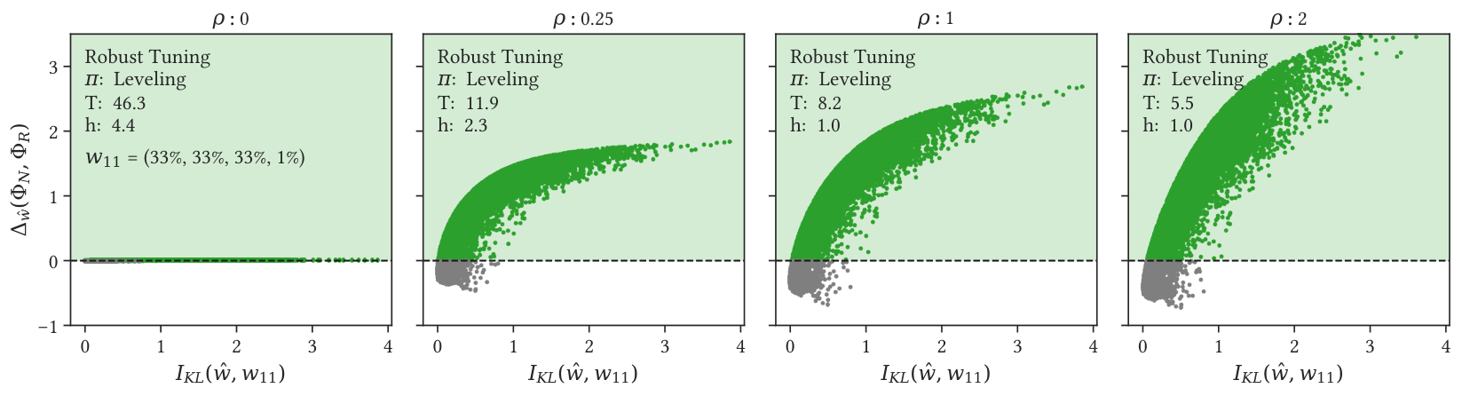
Comparison of Tunings. First, we address the question – is it beneficial to adopt robust tunings relative to the nominal tunings? Intuitively, it should be clear that the performance of nominally tuned databases would degrade when the workloads being executed on the database are significantly different from the expected workloads used for tuning. In Figure 4, we present performance comparisons between the robust and the nominal tunings for different values of uncertainty parameter . We observe that robust tunings provide substantial benefit in terms of normalized delta throughput for unimodal, bimodal, and trimodal workloads. The normalized delta throughput shows over 95% improvement on average over all for robust tunings with , when the expected workload used during tuning belongs to one of these categories. For uniform expected workload, we observe that the nominal tuning outperforms the robust tuning by a modest 5%.
Intuitively, unbalanced workloads result in overfit nominal tunings. Hence, even small variations in the observed workload can lead to significant degradation in the throughput of such nominally tuned databases. On the other hand, robust tunings by their very nature take into account such variations and comprehensively outperform the nominal tunings. In the case of the uniform expected workload , Figure 3 shows us that instances of high values of KL-divergence are extremely rare. In this case, when tuned for high values of , the robust tunings are unrealistically pessimistic and lose out some performance relative to the nominal tuning.
Impact of Tuning Parameter . Next, we address the question – how does the uncertainty tuning parameter impact the performance of the robust tunings? In Figure 5, we take a deep dive into the performance of robust tunings for an individual expected workload for different values of . We observe that the robust tunings for i.e., zero uncertainty, are very close to the nominal tunings. As the value of increases, its performance advantage over the nominal tuning for the observed workloads with higher KL-divergence w.r.t. expected workload increases. Furthermore, the robustness of such configurations have logically sound explanations. The expected workload in Figure 5 consists of just 1% writes. Hence, for low values of , the robust tuning has higher size-ratio leading to shallower LSM trees to achieve good read performance. For higher values of , the robust tunings anticipate an increasing percentage of write queries and hence limit the size-ratio to achieve higher throughput.
In Figure 6, we show the impact of tuning parameter on the throughput range. In Figure 6(a) we plot a histogram of the nominal and robust throughputs for workload . As the value of increases, the interval size between the lowest and the highest throughputs for the robust tunings consistently decreases. We provide further evidence of this phenomenon in Figure 6(b), by plotting the decreasing throughput range averaged across all the expected workloads. Thus, robust tunings not only provide a higher average throughput over all , but they have a more consistent performance (lower variance) compared to the nominal tunings.
How to Choose . Now, we address the question – What is the appropriate choice for the value of uncertainty parameter ? We provide guidance on the choice of in absence of perfect knowledge regarding the future workloads that are likely to be executed on the database. Intuitively, we expect the robust tunings to be only weak when they are tuned for either too little or too much uncertainty. In Figure 7, we explore the relationship between and the KL-divergence for , by making a contour plot of the corresponding normalized delta throughput . We confirm our intuition that nominal tunings compare favorably with our proposed robust tunings only in two scenarios viz., (1) when observed workloads are extremely similar to the expected workload (close to zero observed uncertainty), and (2) when the robust tunings assume extremely low uncertainty with while the observed variation is higher. Based on this evidence, we can advise a potential database administrator that mean KL-divergences between pairs of historically observed workloads would be a reasonable value of while deploying robust tunings in practice.

8. System-Based Evaluation
In this section, we deploy Endure as the tuner of the state-of-the-art LSM-based engine RocksDB, and we show that RocksDB achieves up to 90% lower workload latency in the presence of uncertainty. We further show that the tuning cost is negligible, and the effectiveness of Endure is not affected by data size.
8.1. Experimental Setup & Measurements
Our server is configured with two Intel Xeon Gold 6230 processors, 384 GB of main memory, a 1 TB Dell P4510 NVMe drive, CentOS 7.9.2009, and a default page size of 4 KB. We use Facebook’s RocksDB, a popular LSM tree-based storage system, to evaluate our approach (Facebook [n. d.]). While RocksDB provides implementations of leveling and tiering policies, the system implements micro-optimizations not common across all LSM tree-based storage engines. Therefore, we use RocksDB’s event hooks to implement both classic leveling and tiering policies to benchmark the common compaction strategies (RocksDB 2020a). Following the Monkey memory allocation scheme (Dayan et al. 2017), we allocate different bits per element for Bloom filters per level. To obtain an accurate count of block accesses we enable direct I/Os for both queries and compaction and disable the block cache. The remaining parameters such as buffer size are set by the tuning.
Empirical Measurements. We use the internal RocksDB statistics module to measure the number of logical block accesses during reads, bytes flushed during writes, and bytes read and written in compactions. The number of logical blocks accessed during writes is calculated by dividing the number of bytes reported by the default page size. To estimate the amortized cost of writes, we compute the I/Os from compactions across all workloads of a session and redistribute them across write queries. Our approach of measuring average I/Os per query allows us to compare the effects of different tuning configurations, while simultaneously minimizing the effects of extraneous factors on the database performance.
8.2. Experiment Design
To evaluate the performance of our proposed robust tuning approach, we create multiple instances of RocksDB using different tunings and empirically measure their performance by executing workloads from the uncertainty benchmark . To measure the steady-state performance of the database, each instantiation is initially bulk loaded with the exact same sequence of 10 million unique key-value pairs each of size 1 KB. Each key-value entry has a 16-bit uniformly at random sampled key, with the remaining bits being allocated to a randomly generated value.
While evaluating the performance of the database, we sample a sequence of workloads from the benchmark set . Each sequence is cataloged into one of the categories — expected, empty read, non-empty read, read, range, and write — based on the dominant query type in the workloads in the sequence. Specifically, the expected session contains workloads with a KL-divergence less than 0.2 w.r.t. the expected workload used for tuning. In all other sessions, the dominant query type encompasses 80% of the total queries in the session. The remaining 20% of queries may belong to any of the query types. While generating keys of the queries to run on the database, we ensure that non-empty point reads query a key that exists in the database, while the empty point reads query a key that is not present in the database but is sampled from the same domain. All range queries are generated with minimal selectivity to act as short range queries reading on average zero to two pages per level. Lastly, write queries consist of randomly generated keys that are guaranteed to be unique from the existing keys in the database. Initializing RocksDB and bulk loading requires 30 minutes, while execution of individual workloads are 5 minutes on average.
8.3. Experimental Results
In this section, we replicate key insights from Section 7, evaluate system performance, and show that Endure scales with database size. Due to space constraints, we present results for 2 representative expected workloads, and . An interested reader can find results for all workloads in an extended version of this work (Huynh et al. 2021).
Cost of Tuning. For every experiment, we perform either the nominal or the robust tuning prior to the experiments. Both nominal and robust tuning takes less than 10ms, which is negligible w.r.t. the workload execution time.
Read Performance. We begin by examining the system performance and verifying that the model-predicted I/O and the system-measured I/O match when considering read queries in Figures 8 and 9. In both figures, we include the model-predicted I/Os per query (top), the I/Os per query measured on the system (middle), and the system latency (bottom), for both nominal and robust tunings across different read sessions. The empirical measurements confirm the cost model predictions and show that the predicted performance benefits from the model translate to similar performance benefits in practice. Note that the discrepancy observed between the relative performance between the nominal and the robust tunings in the presence of range queries (session 2 in Figure 8) is due to the fence pointers in RocksDB. The analytical model does not account for fence pointers allowing the system to completely skip a run, which may reduce the measured I/Os for short range queries compared to the predicted I/Os.
Write Performance. In presence of writes (Figures 10 and 11), the model is still predicting the disk accesses successfully and Endure leads to significant performance benefits as expected from the model-based analysis. Note that now the structure of the LSM tree is continually changing across all sessions due to the compactions caused by write queries. For example, the dips in measured I/Os in the range query session in Figure 10 are the result of compactions triggered by write queries in preceding workloads leading to empty levels. Additionally, writes may appear instantaneous w.r.t. system latency as seen in Figure 10 due to RocksDB assigning compactions to background threads. For Figure 10, we see that the particular tuning causes compactions to be fast enough and not stall any future queries. Thus, RocksDB does not experience any latency disruptions in performance. In contrast, in Figure 11 we see that the nominal tuning causes compactions to be costly as the large size-ratio leads to a shallow tree with extremely large levels. Thus, a compaction occurring in the write query dominated session triggers a sort at the lower levels of the tree resulting in a higher number of I/Os than predicted by the model. As a result, we observe that robust tuning reduces I/O and latency by up to . Overall, Figures 8–11 confirm that our analytical model can accurately capture the relative performance of different tunings.
Uniform Workload. In Figure 12 we show an instance where the expected workload and the observed workload are similar (), and we assign the correct . Note that both the robust and nominal tuning produce similar designs. This similarly is reflected in performance, where we see both tunings producing similar system I/O and latency measurements. The only different appears in the writes, session 5, where we observe the nominal tuning causes system to issue more I/Os. Because the nominal design issues more bits per elements to the bloom filter, the memory buffer is smaller implying more compactions are triggered.
Unimodal Workloads. In Figures 13 and 14 we show results for the unimodal workloads. Note that, similar to the previous graphs, when introducing writes into the workload the latency may appear instantaneous as compactions are issued on background threads. We see for the system I/O and model I/O match up well, however, the change in trend for the write session occurs due to the rounding of size ratio. Classical LSM trees cannot have fractional size ratios, therefore we round up when deploying tunings onto the physical system. For we see a similar trend. In we observe that the nominal assigns a large size ratio due to the expectation of range queries being the majority query type. Once a heavy write session occurs, we see the tuning performing much worse than the nominal as the compaction costs becomes much more expensive as your size ratio increases. In contrast, we see the nominal performing well in range queries w.r.t. system latency, however, this benefit does not offset the consistency for query response time we see from the robust tuning. Lastly in we see that because the tree structure changes over time in the presence of writes, there’s a dip in measured system I/O and latency. Additionally, we see the baseline for system I/O per query increasing post session 5 as the tree changes shape.
Biomodal Workloads. In Figures 15 and 17 we see the remaining biomodal workloads. For we see similar results as in and as these workloads are read dominated. Tunings for and shows a similar difference in performance as as the expected workload contains a large fraction of range queries. Both tunings for and show the system I/O jumping after the write session. Again, this is due to the structure of the tree changing. Note that in particular shows the mismatch between system and model I/O as our cost model does not account for the changes in tree structure.
Trimodal Workloads. In Figure 18 we show tunings for the remaining trimodal workloads and their performance. Because of the exclusion of range queries in the expected workload, both tunings for see an increase in system I/O and latency in the range query session. However, the robust tuning does significantly better in both measurements as it lowers the bloom filter memory and size ratio. Workloads and shows the robust tuning experiencing a trade-off of slightly worse range query performance compared to the nominal as evident in the range query session. In return, the robust tuning causes the system to issue much less I/Os when a write heavy session occurs.
Robust Outperforms Nominal for Properly Selected . In the model evaluation (Figure 7), we showed that robust tuning outperforms the nominal tuning in the presence of uncertainty for tuning parameter approximately greater than 0.2. This is further supported by all the system experiments described. We see the analysis of workload tunings above show instances where the KL-divergence of the observed workload averaged across all the sessions w.r.t. the expected workload is close to the tuning parameter . In each of these experiments, the robust tuning outperforms the nominal resulting in up to a reduction in latency and system I/O. Conversely, when the observed workloads are similar to the expected one (), such as in Figure 9, we observe a resulting increase of latency by .
ENDURE Scales with Data Size. To verify that Endure scales, we repeat the previous experiments, while varying the size of the initial database. Each point in Figure 16 is calculated based on a series of workload sessions similar to the ones presented in Figures 9 (11) for the left (right) part of Figure 16. All points use the same expected workload, therefore the nominal and robust tunings are the same across each graph. We observe that the robust and nominal tuning increase buffer memory as the initial database size grows. As a result, for all cases, the number of initial levels is the same regardless of the number of entries. This highlights the importance of the number of levels w.r.t performance. Additionally, the performance gap between robust and nominal stas consistent as database size grows, showing Endure is effective regardless of data size.
8.4. Robustness is All You Need
One of the key challenges during the evaluation of tuning configurations in presence of uncertainty is the challenge in measuring steady-state performance. In Section 8.3, we show that the cost-model can accurately predict the empirical measurements. In the course of this study, using our model, we compared over 700 different robust tunings with their nominal counterparts over the uncertainty benchmark set , leading to approximately 8.6 million comparisons. Robust tunings comprehensively outperform the nominal tunings in over 80% of these comparisons. We further cross-validated the relative performance of the nominal and the robust tunings in over 300 comparisons using RocksDB. The empirical measurements overwhelmingly confirmed the validity of our analytical models, and the few instances of discrepancy in the scale of measured I/Os, such as the ones discussed in previous sections, are easily explained based on the structure of the LSM tree.
Leveling is “more” Robust than Tiering. One of the key takeaways of applying robust tuning to LSM trees is that leveling is inherently more robust to perturbations in workloads when compared to pure tiering. This observation is in line with the industry practice of deploying leveling or hybrid leveling over pure tiering. Overall, based on our analytical and empirical results, the robust tuning should always be employed when tuning an LSM tree, unless the future workload distribution is known with absolute certainty.
Discussion. While we have deployed and tested robust tuning on LSM trees, the robust paradigm of Endure is a generalization of a minimization problem that is at the heart of any database tuning problem. Hence, similar robust optimization approaches can be applied to any database tuning problem assuming that the underlying cost-model is known, and each cost-model component is convex or can be accurately approximated by a convex surrogate.
9. Related Work
Tuning Data Systems. Database systems are notorious for having numerous tuning knobs. These tuning knobs control fine-grained decisions (e.g., number of threads, amount of memory for bufferpool, storage size for logging) as well as basic architectural and physical design decisions about partitioning, index design, materialized views that affect storage and access patterns, and query execution (Bruno and Chaudhuri 2005; Chaudhuri and Narasayya 1998). The database research community has developed several tools to deal with such tuning problems. These tools can be broadly classified as offline workload analysis for index and views design (Agrawal et al. 2004; Agrawal et al. 2000; Chaudhuri and Narasayya 1997; Dageville et al. 2004; Valentin et al. 2000; Zilio et al. 2004), and periodic online workload analysis (Bruno and Chaudhuri 2006; Schnaitter et al. 2006; Schnaitter et al. 2007; Schnaitter and Polyzotis 2012) to capture workload drift (Holze et al. 2010). In addition, there has been research on reducing the magnitude of the search space of tuning (Bruno and Chaudhuri 2005; Dash et al. 2011) and on deciding the optional data partitioning (Athanassoulis et al. 2019; Papadomanolakis and Ailamaki 2004; Serafini et al. 2016; Sun et al. 2014; Sun et al. 2016). These approaches assume that the input information about resources and workload is accurate. When it is proved to be inaccurate, performance is typically severely impacted.
Adaptive & Self-designing Data Systems. A first attempt to address this problem was the design of adaptive systems which had to pay additional transition costs (e.g., when deploying a new tuning) to accommodate shifting workloads (Idreos et al. 2007; Graefe and Kuno 2010a; Graefe and Kuno 2010b; Schuhknecht et al. 2018). More recently the research community has focused on using machine learning to learn the interplay of tuning knobs, and especially of the knobs that are hard to analytically model to perform cost-based optimization. This recent work on self-driving database systems (Aken et al. 2017; Ma et al. 2018; Pavlo et al. 2017) or self-designing database systems (Idreos et al. 2019; Idreos and Kraska 2019; Idreos et al. 2018a; Idreos et al. 2018b) is exploiting new advancements in machine learning to tune database systems and reduce the need for human intervention, however, they also yield suboptimal results when the workload and resource availability information is inaccurate.
Robust Database Physical Design. One of the key database tuning decisions is physical design, that is, the decision of which set of auxiliary structures should be used to allow for the fastest execution of future queries. Most of the existing systems use past workload information as a representative sample for future workloads, which often leads to sub-optimal decisions when there is significant workload drift. Cliffguard (Mozafari et al. 2015) is the first attempt to use unconstrained robust optimization to find a robust physical design. Their method is derived from Bertsimas et al. in (Bertsimas et al. 2010b), a numerical optimization approach using alternating gradient ascent-descent to optimize problems without closed-form objectives. In contrast to Cliffguard, Endure focuses on the LSM tree tuning problem which uses an analytical closed form objective in Equation (2). This allows us to directly solve a Lagrangian dual problem instead of relying upon numerical optimization techniques. Furthermore, we found that the approach in Cliffguard, when applied to our objective, fails to converge even after extensive hyperparameter search.
10. Conclusion
In this work, we explored the impact of workload uncertainty on the performance of LSM tree-based databases, and introduced Endure, a robust tuning paradigm that recommends optimal designs to mitigate any performance degradation in the presence of workload uncertainty. We showed that in the presence of uncertainty, robust tunings increase database throughput compared to standard tunings by up to . Additionally, we provided evidence that our analytical model closely matches the behavior measured on a database system. Through both model-based and extensive experimental evaluation of Endure within the state-of-the-art LSM-based storage engine, RocksDB, we show that the robust tuning methodology consistently outperforms classical tuning strategies. Endure can be used as an indispensable tool for database administrators to both evaluate the performance of tunings, and recommend optimal tunings in a few seconds without resorting to expensive database experiments.
References
- (1)
- Absalyamov et al. (2018) Ildar Absalyamov, Michael J Carey, and Vassilis J Tsotras. 2018. Lightweight Cardinality Estimation in LSM-based Systems. In Proceedings of the ACM SIGMOD International Conference on Management of Data. 841–855. https://doi.org/10.1145/3183713.3183761
- Agrawal et al. (2004) Sanjay Agrawal, Surajit Chaudhuri, Lubor Kollár, Arunprasad P. Marathe, Vivek R. Narasayya, and Manoj Syamala. 2004. Database Tuning Advisor for Microsoft SQL Server 2005. In Proceedings of the International Conference on Very Large Data Bases (VLDB). 1110–1121.
- Agrawal et al. (2000) Sanjay Agrawal, Surajit Chaudhuri, and Vivek R. Narasayya. 2000. Automated Selection of Materialized Views and Indexes in SQL Databases. In Proceedings of the International Conference on Very Large Data Bases (VLDB). 496–505. http://dl.acm.org/citation.cfm?id=645926.671701
- Aken et al. (2017) Dana Van Aken, Andrew Pavlo, Geoffrey J Gordon, and Bohan Zhang. 2017. Automatic Database Management System Tuning Through Large-scale Machine Learning. In Proceedings of the ACM SIGMOD International Conference on Management of Data. 1009–1024. https://doi.org/10.1145/3035918.3064029
- Alkowaileet et al. (2020) Wail Y Alkowaileet, Sattam Alsubaiee, and Michael J Carey. 2020. An LSM-based Tuple Compaction Framework for Apache AsterixDB. Proceedings of the VLDB Endowment 13, 9 (2020), 1388–1400. http://www.vldb.org/pvldb/vol13/p1388-alkowaileet.pdf
- Alsubaiee et al. (2014) Sattam Alsubaiee, Yasser Altowim, Hotham Altwaijry, Alexander Behm, Vinayak R. Borkar, Yingyi Bu, Michael J. Carey, Inci Cetindil, Madhusudan Cheelangi, Khurram Faraaz, Eugenia Gabrielova, Raman Grover, Zachary Heilbron, Young-Seok Kim, Chen Li, Guangqiang Li, Ji Mahn Ok, Nicola Onose, Pouria Pirzadeh, Vassilis J. Tsotras, Rares Vernica, Jian Wen, and Till Westmann. 2014. AsterixDB: A Scalable, Open Source BDMS. Proceedings of the VLDB Endowment 7, 14 (2014), 1905–1916. https://doi.org/10.14778/2733085.2733096
- Andy Huynh, Harshal A. Chaudhari, Evimaria Terzi, and Manos Athanassoulis (2021) Andy Huynh, Harshal A. Chaudhari, Evimaria Terzi, and Manos Athanassoulis. 2021. Robust LSM Tuning. https://github.com/BU-DiSC/endure
- Apache (2021) Apache. 2021. Cassandra. http://cassandra.apache.org (2021).
- Athanassoulis et al. (2019) Manos Athanassoulis, Kenneth S. Bøgh, and Stratos Idreos. 2019. Optimal Column Layout for Hybrid Workloads. Proceedings of the VLDB Endowment 12, 13 (2019), 2393–2407.
- Ben-Tal et al. (2013a) Aharon Ben-Tal, Dick den Hertog, Anja De Waegenaere, Bertrand Melenberg, and Gijs Rennen. 2013a. Robust Solutions of Optimization Problems Affected by Uncertain Probabilities. Manage. Sci. 59, 2 (Feb. 2013), 341–357. https://doi.org/10.1287/mnsc.1120.1641
- Ben-Tal et al. (2013b) Aharon Ben-Tal, Dick den Hertog, Anja De Waegenaere, Bertrand Melenberg, and Gijs Rennen. 2013b. Robust Solutions of Optimization Problems Affected by Uncertain Probabilities. Management Science 59, 2 (2013), 341–357. https://doi.org/10.1287/mnsc.1120.1641
- Ben-Tal and Nemirovski (1998) Aharon Ben-Tal and Arkadi Nemirovski. 1998. Robust Convex Optimization. Mathematics of Operations Research 23, 4 (1998), 769–805. https://doi.org/10.1287/moor.23.4.769
- Bertsimas et al. (2010a) Dimitris Bertsimas, Omid Nohadani, and Kwong Meng Teo. 2010a. Robust Optimization for Unconstrained Simulation-Based Problems. Operations Research 58, 1 (2010), 161–178. https://doi.org/10.1287/opre.1090.0715
- Bertsimas et al. (2010b) Dimitris Bertsimas, Omid Nohadani, and Kwong Meng Teo. 2010b. Robust Optimization for Unconstrained Simulation-Based Problems. Oper. Res. 58, 1 (Feb. 2010), 161–178.
- Bloom (1970) Burton H Bloom. 1970. Space/Time Trade-offs in Hash Coding with Allowable Errors. Commun. ACM 13, 7 (1970), 422–426. http://dl.acm.org/citation.cfm?id=362686.362692
- Bortnikov et al. (2018) Edward Bortnikov, Anastasia Braginsky, Eshcar Hillel, Idit Keidar, and Gali Sheffi. 2018. Accordion: Better Memory Organization for LSM Key-Value Stores. Proceedings of the VLDB Endowment 11, 12 (2018), 1863–1875. http://www.vldb.org/pvldb/vol11/p1863-bortnikov.pdf
- Bruno and Chaudhuri (2005) Nicolas Bruno and Surajit Chaudhuri. 2005. Automatic physical database tuning. In Proceedings of the ACM SIGMOD International Conference on Management of Data. 227–238. https://doi.org/10.1145/1066157.1066184
- Bruno and Chaudhuri (2006) Nicolas Bruno and Surajit Chaudhuri. 2006. To Tune or not to Tune? A Lightweight Physical Design Alerter. In Proceedings of the International Conference on Very Large Data Bases (VLDB). 499–510. http://dl.acm.org/citation.cfm?id=1182635.1164171
- Cao et al. (2020) Zhichao Cao, Siying Dong, Sagar Vemuri, and David H C Du. 2020. Characterizing, Modeling, and Benchmarking RocksDB Key-Value Workloads at Facebook. In Proceedings of the USENIX Conference on File and Storage Technologies (FAST). 209–223.
- Chang et al. (2006) Fay Chang, Jeffrey Dean, Sanjay Ghemawat, Wilson C. Hsieh, Deborah A. Wallach, Mike Burrows, Tushar Chandra, Andrew Fikes, and Robert E. Gruber. 2006. Bigtable: A Distributed Storage System for Structured Data. In Proceedings of the USENIX Symposium on Operating Systems Design and Implementation (OSDI). 205–218. http://dl.acm.org/citation.cfm?id=1267308.1267323
- Chaudhuri et al. (2004) Surajit Chaudhuri, Benoˆit Dageville, and Guy M Lohman. 2004. Self-Managing Technology in Database Management Systems. In Proceedings of the International Conference on Very Large Data Bases (VLDB). 1243. https://doi.org/10.1016/B978-012088469-8.50116-9
- Chaudhuri and Narasayya (1997) Surajit Chaudhuri and Vivek R. Narasayya. 1997. An Efficient Cost-Driven Index Selection Tool for Microsoft SQL Server. In Proceedings of the International Conference on Very Large Data Bases (VLDB). 146–155. http://dl.acm.org/citation.cfm?id=645923.673646
- Chaudhuri and Narasayya (1998) Surajit Chaudhuri and Vivek R Narasayya. 1998. AutoAdmin ’What-if’ Index Analysis Utility. In Proceedings of the ACM SIGMOD International Conference on Management of Data. 367–378. https://doi.org/10.1145/276304.276337
- Chaudhuri and Weikum (2005) Surajit Chaudhuri and Gerhard Weikum. 2005. Foundations of automated database tuning. In Proceedings of the ACM SIGMOD International Conference on Management of Data. 964–965. https://doi.org/10.1145/1066157.1066305
- Chohan et al. (2010) Navraj Chohan, Claris Castillo, Mike Spreitzer, Malgorzata Steinder, Asser N Tantawi, and Chandra Krintz. 2010. See Spot Run: Using Spot Instances for MapReduce Workflows. In Proceedings of USENIX Workshop on Hot Topics in Cloud Computing (HotCloud).
- Dageville et al. (2004) Benoit Dageville, Dinesh Das, Karl Dias, Khaled Yagoub, Mohamed Zait, and Mohamed Ziauddin. 2004. Automatic SQL tuning in oracle 10g. In Proceedings of the International Conference on Very Large Data Bases (VLDB). 1098–1109. http://dl.acm.org/citation.cfm?id=1316689.1316784
- Dash et al. (2011) Debabrata Dash, Neoklis Polyzotis, and Anastasia Ailamaki. 2011. CoPhy: A Scalable, Portable, and Interactive Index Advisor for Large Workloads. Proceedings of the VLDB Endowment 4, 6 (2011), 362–372. https://doi.org/10.14778/1978665.1978668
- Dayan et al. (2017) Niv Dayan, Manos Athanassoulis, and Stratos Idreos. 2017. Monkey: Optimal Navigable Key-Value Store. In Proceedings of the ACM SIGMOD International Conference on Management of Data. 79–94. https://doi.org/10.1145/3035918.3064054
- Dayan et al. (2018) Niv Dayan, Manos Athanassoulis, and Stratos Idreos. 2018. Optimal Bloom Filters and Adaptive Merging for LSM-Trees. ACM Transactions on Database Systems (TODS) 43, 4 (2018), 16:1–16:48. https://doi.org/10.1145/3276980
- Dayan and Idreos (2018) Niv Dayan and Stratos Idreos. 2018. Dostoevsky: Better Space-Time Trade-Offs for LSM-Tree Based Key-Value Stores via Adaptive Removal of Superfluous Merging. In Proceedings of the ACM SIGMOD International Conference on Management of Data. 505–520. https://doi.org/10.1145/3183713.3196927
- Dayan and Idreos (2019) Niv Dayan and Stratos Idreos. 2019. The Log-Structured Merge-Bush & the Wacky Continuum. In Proceedings of the ACM SIGMOD International Conference on Management of Data (SIGMOD). 449–466. https://doi.org/10.1145/3299869.3319903
- DeCandia et al. (2007) Giuseppe DeCandia, Deniz Hastorun, Madan Jampani, Gunavardhan Kakulapati, Avinash Lakshman, Alex Pilchin, Swaminathan Sivasubramanian, Peter Vosshall, and Werner Vogels. 2007. Dynamo: Amazon’s Highly Available Key-value Store. ACM SIGOPS Operating Systems Review 41, 6 (2007), 205–220. https://doi.org/10.1145/1323293.1294281
- Dong et al. (2017) Siying Dong, Mark Callaghan, Leonidas Galanis, Dhruba Borthakur, Tony Savor, and Michael Strum. 2017. Optimizing Space Amplification in RocksDB. In Proceedings of the Biennial Conference on Innovative Data Systems Research (CIDR). http://cidrdb.org/cidr2017/papers/p82-dong-cidr17.pdf
- Facebook ([n. d.]) Facebook. [n. d.]. MyRocks. http://myrocks.io/ ([n. d.]).
- Facebook (2021) Facebook. 2021. RocksDB. https://github.com/facebook/rocksdb (2021).
- Galante and Bona (2012) Guilherme Galante and Luis Carlos Erpen De Bona. 2012. A Survey on Cloud Computing Elasticity. In Proceedings of the IEEE International Conference on Utility and Cloud Computing (UCC). 263–270. https://doi.org/10.1109/UCC.2012.30
- Google (2021) Google. 2021. LevelDB. https://github.com/google/leveldb/ (2021).
- Graefe and Kuno (2010a) Goetz Graefe and Harumi Kuno. 2010a. Self-selecting, self-tuning, incrementally optimized indexes. In Proceedings of the International Conference on Extending Database Technology (EDBT). 371–381. http://dl.acm.org/citation.cfm?id=1739041.1739087
- Graefe and Kuno (2010b) Goetz Graefe and Harumi A. Kuno. 2010b. Adaptive indexing for relational keys. In Proceedings of the IEEE International Conference on Data Engineering Workshops (ICDEW). 69–74.
- Hayes (2008) Brian Hayes. 2008. Cloud computing. Commun. ACM 51, 7 (2008), 9–11. https://doi.org/10.1145/1364782.1364786
- HBase (2013) HBase. 2013. Online reference. http://hbase.apache.org/ (2013).
- Herbst et al. (2013) Nikolas Roman Herbst, Samuel Kounev, and Ralf H Reussner. 2013. Elasticity in Cloud Computing: What It Is, and What It Is Not. In Proceedings of the International Conference on Autonomic Computing (ICAC). 23–27.
- Holze et al. (2010) Marc Holze, Ali Haschimi, and Norbert Ritter. 2010. Towards workload-aware self-management: Predicting significant workload shifts. Proceedings of the IEEE International Conference on Data Engineering (ICDE) (2010), 111–116. https://doi.org/10.1109/ICDEW.2010.5452738
- Huang et al. (2019) Gui Huang, Xuntao Cheng, Jianying Wang, Yujie Wang, Dengcheng He, Tieying Zhang, Feifei Li, Sheng Wang, Wei Cao, and Qiang Li. 2019. X-Engine: An Optimized Storage Engine for Large-scale E-commerce Transaction Processing. In Proceedings of the ACM SIGMOD International Conference on Management of Data. 651–665. https://doi.org/10.1145/3299869.3314041
- Huynh et al. (2021) Andy Huynh, Harshal Chaudhari, Evimaria Terzi, and Manos Athanassoulis. 2021. Endure: A Robust Tuning Paradigm for LSM Trees Under Workload Uncertainty. arXiv:2110.13801
- Idreos et al. (2019) Stratos Idreos, Niv Dayan, Wilson Qin, Mali Akmanalp, Sophie Hilgard, Andrew Ross, James Lennon, Varun Jain, Harshita Gupta, David Li, and Zichen Zhu. 2019. Design Continuums and the Path Toward Self-Designing Key-Value Stores that Know and Learn. In Proceedings of the Biennial Conference on Innovative Data Systems Research (CIDR).
- Idreos et al. (2007) Stratos Idreos, Martin L. Kersten, and Stefan Manegold. 2007. Database Cracking. In Proceedings of the Biennial Conference on Innovative Data Systems Research (CIDR).
- Idreos and Kraska (2019) Stratos Idreos and Tim Kraska. 2019. From Auto-tuning One Size Fits All to Self-designed and Learned Data-intensive Systems. In Proceedings of the ACM SIGMOD International Conference on Management of Data (SIGMOD).
- Idreos et al. (2018a) Stratos Idreos, Kostas Zoumpatianos, Manos Athanassoulis, Niv Dayan, Brian Hentschel, Michael S. Kester, Demi Guo, Lukas M. Maas, Wilson Qin, Abdul Wasay, and Yiyou Sun. 2018a. The Periodic Table of Data Structures. IEEE Data Engineering Bulletin 41, 3 (2018), 64–75. http://sites.computer.org/debull/A18sept/p64.pdf
- Idreos et al. (2018b) Stratos Idreos, Kostas Zoumpatianos, Brian Hentschel, Michael S Kester, and Demi Guo. 2018b. The Data Calculator: Data Structure Design and Cost Synthesis from First Principles and Learned Cost Models. In Proceedings of the ACM SIGMOD International Conference on Management of Data. 535–550. https://doi.org/10.1145/3183713.3199671
- influxdata ([n. d.]) influxdata. [n. d.]. Online reference. https://www.influxdata.com/ ([n. d.]).
- Intel (2011) Intel. 2011. Best Practices for Building an Enterprise Private Cloud. White Paper (2011).
- Kim et al. (2020) Taewoo Kim, Alexander Behm, Michael Blow, Vinayak Borkar, Yingyi Bu, Michael J. Carey, Murtadha Hubail, Shiva Jahangiri, Jianfeng Jia, Chen Li, Chen Luo, Ian Maxon, and Pouria Pirzadeh. 2020. Robust and efficient memory management in Apache AsterixDB. Software - Practice and Experience 50, 7 (2020), 1114–1151. https://doi.org/10.1002/spe.2799
- Kullback et al. (1951) Solomon Kullback, M Kupperman, and H H Ku. 1951. Tests for Contingency Tables and Markov Chains. Technometrics 4, 4 (1951), 573–708. http://www.jstor.org/stable/1266291
- Luo (2020) Chen Luo. 2020. Breaking Down Memory Walls in LSM-based Storage Systems. In Proceedings of the ACM SIGMOD International Conference on Management of Data. 2817–2819. https://doi.org/10.1145/3318464.3384399
- Luo and Carey (2019) Chen Luo and Michael J Carey. 2019. On Performance Stability in LSM-based Storage Systems. Proceedings of the VLDB Endowment 13, 4 (2019), 449–462.
- Luo and Carey (2020) Chen Luo and Michael J. Carey. 2020. LSM-based Storage Techniques: A Survey. The VLDB Journal 29, 1 (2020), 393–418. https://doi.org/10.1007/s00778-019-00555-y
- Luo et al. (2019) Chen Luo, Pinar Tözün, Yuanyuan Tian, Ronald Barber, Vijayshankar Raman, and Richard Sidle. 2019. Umzi: Unified Multi-Zone Indexing for Large-Scale HTAP. In Proceedings of the International Conference on Extending Database Technology (EDBT). 1–12. https://doi.org/10.5441/002/edbt.2019.02
- Luo et al. (2020) Siqiang Luo, Subarna Chatterjee, Rafael Ketsetsidis, Niv Dayan, Wilson Qin, and Stratos Idreos. 2020. Rosetta: A Robust Space-Time Optimized Range Filter for Key-Value Stores. In Proceedings of the ACM SIGMOD International Conference on Management of Data. 2071–2086. https://doi.org/10.1145/3318464.3389731
- Ma et al. (2018) Lin Ma, Dana Van Aken, Ahmed Hefny, Gustavo Mezerhane, Andrew Pavlo, and Geoffrey J Gordon. 2018. Query-based Workload Forecasting for Self-Driving Database Management Systems. In Proceedings of the ACM SIGMOD International Conference on Management of Data. 631–645. https://doi.org/10.1145/3183713.3196908
- Mohan (2016) C Mohan. 2016. Hybrid Transaction and Analytics Processing (HTAP): State of the Art. In Proceedings of the International Workshop on Business Intelligence for the Real-Time Enterprise (BIRTE).
- Mozafari et al. (2015) Barzan Mozafari, Eugene Zhen Ye Goh, and Dong Young Yoon. 2015. CliffGuard: A Principled Framework for Finding Robust Database Designs. In Proceedings of the ACM SIGMOD International Conference on Management of Data. 1167–1182. https://doi.org/10.1145/2723372.2749454
- O’Neil et al. (1996) Patrick E. O’Neil, Edward Cheng, Dieter Gawlick, and Elizabeth J. O’Neil. 1996. The log-structured merge-tree (LSM-tree). Acta Informatica 33, 4 (1996), 351–385. http://dl.acm.org/citation.cfm?id=230823.230826
- Özcan et al. (2017) Fatma Özcan, Yuanyuan Tian, and Pinar Tözün. 2017. Hybrid Transactional/Analytical Processing: A Survey. In Proceedings of the ACM SIGMOD International Conference on Management of Data. 1771–1775. https://doi.org/10.1145/3035918.3054784
- Papadomanolakis and Ailamaki (2004) Stratos Papadomanolakis and Anastasia Ailamaki. 2004. AutoPart: Automating Schema Design for Large Scientific Databases Using Data Partitioning. In Proceedings of the International Conference on Scientific and Statistical Database Management (SSDBM). 383. https://doi.org/10.1109/SSDBM.2004.19
- Pardo (2018) Leandro Pardo. 2018. Statistical Inference Based on Divergence Measures. Chapman and Hall/CRC. https://doi.org/10.1201/9781420034813
- Pavlo et al. (2017) Andrew Pavlo, Gustavo Angulo, Joy Arulraj, Haibin Lin, Jiexi Lin, Lin Ma, Prashanth Menon, Todd C Mowry, Matthew Perron, Ian Quah, Siddharth Santurkar, Anthony Tomasic, Skye Toor, Dana Van Aken, Ziqi Wang, Yingjun Wu, Ran Xian, and Tieying Zhang. 2017. Self-Driving Database Management Systems. In Proceedings of the Biennial Conference on Innovative Data Systems Research (CIDR). http://cidrdb.org/cidr2017/papers/p42-pavlo-cidr17.pdf
- Pezzini et al. (2014) Massimo Pezzini, Donald Feinberg, Nigel Rayner, and Roxane Edjlali. 2014. Hybrid Transaction/Analytical Processing Will Foster Opportunities for Dramatic Business Innovation. https://www.gartner.com/doc/2657815/ (2014). https://www.gartner.com/doc/2657815/
- Ren et al. (2017) Kai Ren, Qing Zheng, Joy Arulraj, and Garth Gibson. 2017. SlimDB: A Space-Efficient Key-Value Storage Engine For Semi-Sorted Data. Proceedings of the VLDB Endowment 10, 13 (2017), 2037–2048. http://www.vldb.org/pvldb/vol10/p2037-ren.pdf
- Research (2019) Grand View Research. 2019. Private Cloud Server Market Size, Share & Trend Analysis Report By Hosting Type (User Hosting, Provider Hosting), By Organization Type (SME, Large Enterprise), By Region, And Segment Forecasts, 2019 - 2025. White Paper (2019).
- RocksDB (2020a) RocksDB. 2020a. Leveled Compaction. https://github.com/facebook/rocksdb/wiki/Leveled-Compaction (2020).
- RocksDB (2020b) RocksDB. 2020b. Universal Compaction. https://github.com/facebook/rocksdb/wiki/Universal-Compaction (2020).
- Sarkar et al. (2020) Subhadeep Sarkar, Tarikul Islam Papon, Dimitris Staratzis, and Manos Athanassoulis. 2020. Lethe: A Tunable Delete-Aware LSM Engine. In Proceedings of the ACM SIGMOD International Conference on Management of Data. 893–908. https://doi.org/10.1145/3318464.3389757
- Sarkar et al. (2021) Subhadeep Sarkar, Dimitris Staratzis, Zichen Zhu, and Manos Athanassoulis. 2021. Constructing and Analyzing the LSM Compaction Design Space. Proceedings of the VLDB Endowment 14, 11 (2021), 2216–2229. http://vldb.org/pvldb/vol14/p2216-sarkar.pdf
- Schnaitter et al. (2006) Karl Schnaitter, Serge Abiteboul, Tova Milo, and Neoklis Polyzotis. 2006. COLT: Continuous On-Line Database Tuning. In Proceedings of the ACM SIGMOD International Conference on Management of Data. 793–795. https://doi.org/10.1145/1142473.1142592
- Schnaitter et al. (2007) Karl Schnaitter, Serge Abiteboul, Tova Milo, and Neoklis Polyzotis. 2007. On-Line Index Selection for Shifting Workloads. In Proceedings of the IEEE International Conference on Data Engineering Workshops (ICDEW). 459–468. https://doi.org/10.1109/ICDEW.2007.4401029
- Schnaitter and Polyzotis (2012) Karl Schnaitter and Neoklis Polyzotis. 2012. Semi-automatic index tuning. Proceedings of the VLDB Endowment 5, 5 (2012), 478–489. https://doi.org/10.14778/2140436.2140444
- Schuhknecht et al. (2018) Felix Martin Schuhknecht, Jens Dittrich, and Laurent Linden. 2018. Adaptive Adaptive Indexing. In Proceedings of the IEEE International Conference on Data Engineering (ICDE). 665–676. https://doi.org/10.1109/ICDE.2018.00066
- Serafini et al. (2016) Marco Serafini, Rebecca Taft, Aaron J Elmore, Andrew Pavlo, Ashraf Aboulnaga, and Michael Stonebraker. 2016. Clay: Fine-Grained Adaptive Partitioning for General Database Schemas. Proceedings of the VLDB Endowment 10, 4 (2016), 445–456. http://www.vldb.org/pvldb/vol10/p445-serafini.pdf
- Shasha and Bonnet (2002) Dennis E Shasha and Philippe Bonnet. 2002. Database Tuning: Principles, Experiments, and Troubleshooting Techniques. In Proceedings of the International Conference on Very Large Data Bases (VLDB).
- Sun et al. (2014) Liwen Sun, Michael J. Franklin, Sanjay Krishnan, and Reynold S. Xin. 2014. Fine-grained Partitioning for Aggressive Data Skipping. In Proceedings of the ACM SIGMOD International Conference on Management of Data. 1115–1126. https://doi.org/10.1145/2588555.2610515
- Sun et al. (2016) Liwen Sun, Michael J. Franklin, Jiannan Wang, and Eugene Wu. 2016. Skipping-oriented Partitioning for Columnar Layouts. Proceedings of the VLDB Endowment 10, 4 (2016), 421–432. http://www.vldb.org/pvldb/vol10/p421-sun.pdf
- Tarkoma et al. (2012) Sasu Tarkoma, Christian Esteve Rothenberg, and Eemil Lagerspetz. 2012. Theory and Practice of Bloom Filters for Distributed Systems. IEEE Communications Surveys & Tutorials 14, 1 (2012), 131–155. http://ieeexplore.ieee.org/xpl/login.jsp?arnumber=5751342
- Valentin et al. (2000) Gary Valentin, Michael Zuliani, Daniel C. Zilio, Guy M. Lohman, and Alan Skelley. 2000. DB2 Advisor: An Optimizer Smart Enough to Recommend its own Indexes. In Proceedings of the IEEE International Conference on Data Engineering (ICDE). 101–110. http://dx.doi.org/10.1109/ICDE.2000.839397
- Virtanen et al. (2020) Pauli Virtanen, Ralf Gommers, Travis E. Oliphant, Matt Haberland, Tyler Reddy, and et al. Cournapeau, D. 2020. SciPy 1.0: Fundamental Algorithms for Scientific Computing in Python. Nature Methods 17 (2020), 261–272. https://doi.org/10.1038/s41592-019-0686-2
- Wikipedia contributors (2021) Wikipedia contributors. 2021. Bloom filter — Wikipedia, The Free Encyclopedia. https://en.wikipedia.org/w/index.php?title=Bloom_filter&oldid=1025193696. [Online; accessed 8-June-2021].
- WiredTiger (2021) WiredTiger. 2021. Source Code. https://github.com/wiredtiger/wiredtiger (2021).
- Wolski et al. (2017) Rich Wolski, John Brevik, Ryan Chard, and Kyle Chard. 2017. Probabilistic guarantees of execution duration for Amazon spot instances. In Proceedings of the International Conference for High Performance Computing, Networking, Storage and Analysis (SC). 18:1—-18:11. https://doi.org/10.1145/3126908.3126953
- Yang et al. (2020) Lei Yang, Hong Wu, Tieying Zhang, Xuntao Cheng, Feifei Li, Lei Zou, Yujie Wang, Rongyao Chen, Jianying Wang, and Gui Huang. 2020. Leaper: A Learned Prefetcher for Cache Invalidation in LSM-tree based Storage Engines. Proceedings of the VLDB Endowment 13, 11 (2020), 1976–1989.
- Zhang et al. (2018) Huanchen Zhang, Hyeontaek Lim, Viktor Leis, David G Andersen, Michael Kaminsky, Kimberly Keeton, and Andrew Pavlo. 2018. SuRF: Practical Range Query Filtering with Fast Succinct Tries. In Proceedings of the ACM SIGMOD International Conference on Management of Data. 323–336. https://doi.org/10.1145/3183713.3196931
- Zhang et al. (2020a) Huanchen Zhang, Hyeontaek Lim, Viktor Leis, David G Andersen, Michael Kaminsky, Kimberly Keeton, and Andrew Pavlo. 2020a. Succinct Range Filters. ACM Transactions on Database Systems (TODS) 45, 2 (2020), 5:1—-5:31. https://doi.org/10.1145/3375660
- Zhang et al. (2020b) Teng Zhang, Jianying Wang, Xuntao Cheng, Hao Xu, Nanlong Yu, Gui Huang, Tieying Zhang, Dengcheng He, Feifei Li, Wei Cao, Zhongdong Huang, and Jianling Sun. 2020b. FPGA-Accelerated Compactions for LSM-based Key-Value Store. In 18th USENIX Conference on File and Storage Technologies, FAST 2020, Santa Clara, CA, USA, February 24-27, 2020. 225–237.
- Zilio et al. (2004) Daniel C. Zilio, Jun Rao, Sam Lightstone, Guy M. Lohman, Adam Storm, Christian Garcia-Arellano, and Scott Fadden. 2004. DB2 Design Advisor: Integrated Automatic Physical Database Design. In Proceedings of the International Conference on Very Large Data Bases (VLDB). 1087–1097. http://dl.acm.org/citation.cfm?id=1316689.1316783