A Cartesian FMM-accelerated Galerkin boundary integral
Poisson-Boltzmann solver

The PB model for a solvated biomolecule is depicted in Fig. 1(a) in which the molecular surface $\Gamma$ separates the solute domain $\Omega_{1}$ from the solvent domain $\Omega_{2}$. Figure 1(b) is an example of the molecular surface $\Gamma$ as the triangulated surface of protein barstar [45]. In domain $\Omega_{1}$, the solute is represented by $N_{c}$ partial charges $q_{k}$ located at atomic centers ${\bf r}_{k}$ for $k=1,\cdots,N_{c}$, while in domain $\Omega_{2}$, a distribution of ions is described by a Boltzmann distribution and we consider a linearized version in this study. The solute domain has a low dielectric constant $\epsilon_{1}$ and the solvent domain has a high dielectric constant $\epsilon_{2}$. The modified inverse Debye length $\bar{\kappa}$ is given as $\bar{\kappa}^{2}=\epsilon_{2}\kappa^{2}$, where $\kappa$ is the inverse Debye length measuring the ionic strength; $\bar{\kappa}=0$ in $\Omega_{1}$ and is nonzero only in $\Omega_{2}$. The electrostatic potential $\phi({\bf x})$ satisfies the linear PB equation,

subject to continuity conditions for the potential and electric flux density on $\Gamma$,

where $[f]=f_{1}-f_{2}$ is the difference of the quantity $f$ across the interface, and $\phi_{\nu}=\partial\phi/\partial{\nu}$ is the partial derivative in the outward normal direction $\nu$. The model also incorporates the far-field condition,

Note that Eqs. (1)-(3) define a boundary value problem for the potential $\phi({\bf x})$ which in general must be solved numerically.

This section summarizes the well-conditioned boundary integral form of the PB implicit solvent model we employ [25, 31]. Applying Green’s second identity and properties of fundamental solutions to Eq. (1) yields the electrostatic potential in each domain,

where $G_{0}({\bf x},{\bf y})$ and $G_{\kappa}({\bf x},{\bf y})$ are the Coulomb and screened Coulomb potentials,

and ${\bf y}_{k}\in\Omega_{1}$ are the location of the atomic centers.

Applying the interface conditions in Eq. (2) with the differentiation of electrostatic potential in each domain yield a set of boundary integral equations relating the surface potential $\phi_{1}$ (the subscript 1 denotes the inside domain) and its normal derivative $\partial\phi_{1}/\partial{\nu}$ on $\Gamma$, [25, 31],

where $\varepsilon=\varepsilon_{2}/\varepsilon_{1}$, and the kernels $K_{1,2,3,4}$ and source terms $S_{1,2}$ are

and

As given in Eqs. (7a-7b) and (8), the kernels $K_{1,2,3,4}$ and source terms $S_{1,2}$ are linear combinations of $G_{0}$, $G_{k}$, and their first and second order normal derivatives [25, 31]. Since the Coulomb potential is singular, the kernels have the following behavior

as ${\bf y}\to{\bf x}$.

After the potentials $\phi_{1}$ and $\partial\phi_{1}/\partial\nu$ have been found by solving the boundary integral equation, the electrostatic solvation energy can be obtained by

where $\phi_{\rm reac}({\bf x})=\phi_{1}({\bf x})-S_{1}({\bf x})$ is the reaction potential [25, 31].

In solving the boundary integral PB equation, both the molecular surface and the solution function need to be discretized. The molecular surface $\Gamma$ is usually approximated by a collection of triangles

where $N$ is number of elements and $\tau_{i}$ for $i=1,\dots,N$ is a planar triangular boundary element with mid-point $\textbf{x}^{c}_{i}$. This triangulation must be conforming, i.e., the intersection of two different triangles is either empty, or a common vertex or edge. Fortunately, surface generators are available, and our choice for our computations is MSMS [44], though other packages could also be used. Here, the resolution of the surface can be controlled by the parameter $d$ that controls the number of vertices per Ų. For example, Fig. 1 (b) shows the triangulated molecule surface of the protein barstar, which will bind another protein barnase to form a biomolecular complex (PDB: 1b2s) [45].

Each triangle $\tau_{i}$ of $\Gamma_{N}$ is the parametric image of the reference triangle $\tau$

If $\textbf{u}_{i}$, $\textbf{v}_{i}$ and $\textbf{w}_{i}$ are the vertices then the parameterization is given by

The area of the element, the local mesh size, and the global mesh size of the boundary elements $\tau_{i}$ are given as $A_{i}=\frac{1}{2}|(\textbf{v}_{i}-\textbf{u}_{i})\times(\textbf{w}_{i}-\textbf{u}_{i})|$, $h_{i}=\sqrt{A_{i}}$, and $h=\max\limits_{1\leq i\leq N}h_{i}$.

Since a function $f$ defined on $\tau_{i}$ can be interpreted as a function $g(\eta)$ with respect to the reference element $\tau$,

we can define a finite element space by functions on $\Gamma_{N}$ whose pullbacks to the reference triangle are polynomials in $\eta$. The simplest example is the space of piecewise constant functions, which are polynomials of order zero on each triangle, which will be denoted by $S^{0}_{h}(\Gamma_{N})$. Obviously, the dimension of this space is $N$ and the basis is given by the box functions

where $i$ is an index of a triangle.

The next step up are piecewise linear functions. Since there are three independent linear functions on $\tau$, namely,

the dimension is $3N$. Usually, one works with the space of continuous linear functions, denoted by $S^{1}_{h}(\Gamma_{N})$. It is not hard to see that the dimension of this space is the number of vertices and that the basis is given by

where ${v}_{i}$ is the $i$-th vertex.

The approximation powers of piecewise polynomial spaces are well known, see, e.g., [46]. For a function $w\in H^{1}_{pw}(\Gamma_{N})$ we denote by $w_{h}^{0}$ the $L_{2}$-orthogonal projection of $w$ into the space of piecewise constant functions, then

where $c$ is the upper bound of the mesh ratio $h_{\max}/h_{\min}$, $h$ is the maximal diameter of a triangle and

Thus, the constant piecewise basis function can give a convergence rate of maximum $O(h)$.

Likewise, the error for the $L_{2}$-orthogonal projection $w_{h}^{1}$ of $w\in H^{2}_{pw}(\Gamma_{N})$ into $S^{1}_{h}(\Gamma_{N})$ is

Finite element spaces with higher order polynomials could also be considered, however their practical value for surfaces with low regularity and complicated geometries is limited.

The Galerkin discretization is based on a variational formulation of integral equations (6a) and (6b). That is, instead of understanding the equations pointwise for ${\bf x}\in\Gamma_{N}$ the equations are multiplied by test functions $\psi$ and $\psi^{\nu}$ and integrated again over $\Gamma_{N}$. Solving the variational form amounts to finding $\phi_{1}$ and $\partial\phi_{1}/\partial\nu$ such that

holds for all test functions $\psi,\psi^{\nu}$. In the Galerkin method the solution and the test functions are formally replaced by functions in the finite element space. To that end, the unknowns are expanded by basis functions $\psi_{i}$ (which could be either box or hat functions)

and integral equations are tested against the basis functions. This leads to the linear system $Ax=b$ where $x$ contains the coefficients in (21) and

The entries of these block matrices are given as

and the right hand side is

Since the basis functions vanish on most triangles, the integrations for the coefficients are only local. For instance, for piecewise constant elements, the integral $\int_{\Gamma}\dots\psi_{i}dS_{\bf{x}}$ reduces to $\int_{\tau_{i}}\dots dS_{\bf{x}}$. Since the coefficients cannot be expressed in analytical form they have to be calculated by a suitable choice of quadrature rule. However singularities will appear if triangles $\tau_{i}$ and $\tau_{j}$ are identical or sharing common edges and vertices. To overcome this issue, we apply the singularity removing transformation of [47]. This results smooth integrals over a four dimensional cube. The latter integrals are then approximated by tensor product Gauss-Legendre quadrature.

After the solution of the linear system has been obtained, the electrostatic free solvation energy can be calculated using the approximations for the surface potentials and its normal derivative

Since the matrix $A$ is a dense and non-symmetric our choice of solver is the GMRES method. In each step of GMRES iteration, a matrix-vector product is calculated and a direct summation for this requires $O(N^{2})$ complexity. Below we will introduce the $O(N)$ Cartesian Fast Multipole Method (FMM) to accelerate the matrix-vector product. Calculating the electrostatic solvation free energy $E_{sol}$ in Eq. (25) is $O(N_{c}N)$ and we use a Cartesian treecode to reduce the cost to $O(N_{c}\log(N))$. Both FMM and treecode algorithm are described the next for comparison and for the reason that both are used to accelerate the N-body particle-particle interactions.

In this section, we introduce the Cartesian FMM to evaluate matrix vector products with the matrix in (22) efficiently. This is a kernel-independent version of the FMM, where instead of the multipole expansion, truncated Taylor series are used to approximate Coulomb ($\kappa=0$) the screened Coulomb ($\kappa\neq 0$) potential.

This considerably simplifies the translation operators for the kernels $K_{1-4}$ because they involve different values of $\kappa$. It was shown in [48] how the derivatives of the Coulomb kernel can be computed by simple recurrence formulas. Furthermore, the moment-to-moment (MtM) and local-to-local (LtL) translation are easily derived using the binomial formula.

When a refined mesh is required for a larger $N$, increasing the expansion order is essential to control the accuracy. The FMM error analysis implies that the truncated Taylor expansion error has the same magnitude as the discretization error if the expansion order is adjusted to the level according to the formula

where $l=0,1,\cdots,L$ with $l=0$ the coarsest level and $l=L$ the finest level. That is, the finest level uses a low-order expansion $p_{L}$, and the order is incremented in each coarser level, see [35].

Note that the multipole series is more efficient as it contains $(p+1)^{2}$ terms, while the Taylor series has $p(p+1)(p+2)/6$ terms. This difference becomes significant with larger values of $p$. However, with the variable order scheme the advantage of the multipole series is much less because most translation operators are in the fine levels where the number of terms in both series are comparable.

The matrix vector product can be considered as generalized $N$-body problem of the form

where $k,l\in\{0,1\}$ and $f_{h}$ is a linear combination of the basis functions $\psi_{j}$.

Next we show how the Cartesian FMM is used under the framework of boundary element method.

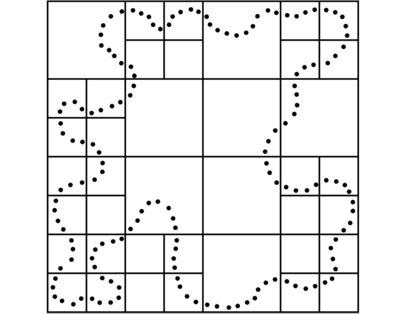
Figure 2a is a 2-D illustration of a discretized molecular surface $\Gamma_{N}$ embedded in a hierarchy of cubes (squares in the image). Each black solid dot represents a boundary triangle $\tau_{i}$ for $i=1,\cdots,N$.

A cluster $c$ in any level $l$ is defined as the union of triangles whose centroid are located in a cube of that level. $C_{l}$ is the set of all clusters in level $l$.

The level-0 cube is the smallest axiparallel cube that contains $\Gamma_{N}$ and thus $C_{0}=\Gamma_{N}$. The refinement of coarser cubes into finer cubes stops when clusters in the finest level contain at most a predetermined (small) number of triangles. For a cluster $c$ we denote by $B_{c}$ the smallest axiparallel rectangular box that contains $c$ and write ${\bf x}_{c}$ for its center and $\rho_{c}$ for the half-length of its longest diagonal. Note that $B_{c}$ can be considerably smaller than its cube, this is why we call this process the shrink scheme. For two clusters $c$ and $c^{\prime}$ in the same level we denote by

the separation ratio of the two clusters. This number determines the convergence rate of the Taylor series expansion, see [35]. Two clusters in the same level are neighbors if their separation ratio is larger than a predetermined constant. $\mathcal{N}(c)$ denotes the set of its neighbors for a given cluster $c$. The set of nonempty children of $c$ that are generated in the refinement process is denoted by $\mathcal{K}(c)$. Finally, we use $\mathcal{I}(c)$ to denote the interaction list for a cluster $c$, which are clusters at the same level such that for any $c^{\prime}\in\mathcal{I}(c)$, the parent of $c^{\prime}$ is a neighbor of the parent of $c$, but $c^{\prime}$ itself is not a neighbor of $c$.

Under the FMM framework, the evaluation of Eq. (27) consists of the near field direct summation and the Taylor expansion approximation for well-separated far field. The near field direct summation happens in between neighboring panels in the finest level. The far field summation is done by multipole or Taylor expansions between interaction lists in all levels. This process is described in many papers, so we do not give details about the derivation.

To emphasize the differences of the cartesian FMM, we consider a cluster-cluster interaction between two clusters $c$ and $c^{\prime}\in\mathcal{I}(c)$. Let $u$ be the potential due to sources in $c^{\prime}$ which is evaluated in $c$, then by Taylor expansion of the kernel with center ${\bf x}={\bf x}_{c}$ and ${\bf y}={\bf x}_{c^{\prime}}$ one finds easily that

where and $\alpha=(\alpha_{1},\alpha_{2},\alpha_{3})\in\mathbb{N}^{3}$ is a multi-index. The expansion coefficients are given by

where $\alpha!=\alpha_{1}!\alpha_{2}!\alpha_{3}!$ and $m^{\beta}_{c^{\prime}}(f)$ is the moment of $f_{h}$, given by

Equation (30) translates the moment of $c^{\prime}$ to the local expansion coefficients of the cluster $c$, and it is therefore called MtL translation. Since $f_{h}$ is a linear combination of basis functions, we obtain from linearity that

where $f_{i}$ are the coefficients of $f_{h}$ with respect to the $\psi_{i}$-basis and the summation is taken over basis functions that whose support overlaps with $c$. Since we consider a Galerkin discretization we have to integrate the function $u_{c,c^{\prime}}({\bf x})$ against the test functions, to obtain the contribution $g_{i}$ of the two clusters to the matrix vector product. Thus we get from (29)

This operation converts expansion coefficients to potentials and is denoted as LtP translation.

To move moments and local expansion coefficients between levels, we also need the moment-to-moment (MtM) and local-to-local (LtL) translations. They can be derived easily from the multivariate binomial formula. We obtain

and

where $c^{\prime}\in\mathcal{K}(c)$.

We see that moments and expansion coefficients are computed by recurrence from the previous level. In the finest level the moments of the basisfunctions $m_{c}(\psi_{i})$ can be either computed by numerical quadrature, or even analytically, because we consider flat panels and polynomial ansatz functions. We skip the details, as these formulas are straightforward application of the binomial formula.

In summary, the Cartesian FMM under the framework of boundary element method is described as the following.

1. 1.

   Nearfield Calculation.
   for $c\in C_{L}$
      for $c^{\prime}\in\mathcal{N}(c)$
       multiply matrix block of $c$ and $c^{\prime}$ directly.

2. 2.

   Moment Calculation.
   for $c\in C_{L}$
      Compute the moments $m^{\beta}_{c^{\prime}}(f)$ in (32).

3. 3.

   Upward Pass.
   for $l=L-1,\dots,l_{min}$
     for $c\in C_{l}$
      for $c^{\prime}\in\mathcal{K}(c)$
         Compute the MtM translation (34)

4. 4.

   Interaction Phase.
   for $l=L,\dots,l_{min}$
      for $\nu\in C_{l}$
       for $\nu^{\prime}\in\mathcal{N}(c)$
         Compute the MtL translation (30)

5. 5.

   Downward Pass.
   for $l=l_{min},\dots,L-1$
      for $c\in C_{l}$
       for $c^{\prime}\in\mathcal{K}(c)$
         Compute the LtL translation (35)

6. 6.

   Evaluation Phase.
   for $c\in C_{L}$
      Compute the LtP translation (33)

In this algorithm $l_{min}$ is the coarsest level that contains clusters with non-empty interaction lists.

Since the finest level contain a fixed number of triangles the number of levels grows logarithmically with $N$ as the mesh is refined. With a geometric series argument, one can show that the total number of interaction lists in all levels is $O(N)$. If the translations in all levels are computed with the same order $p$ then the complexity of all translations is $O(Np^{3})$. If the variable order method is used where the order is given by (26), then the complexity reduces to $O(N)$. More details can be found in  [35].

The Cartesian treecode can be considered as a fast multipole method without the downward pass. The computational cost of treecode is order of $O(N\log N)$ as opposed to the $O(N)$ FMM. However, the constants in this complexity estimate are smaller, and we found it to be useful for the computation of the free solvation energy (25), where the source and evaluation points are different and zero or limited near field calculations are required. The direct computation of the solvation energy as interactions between $N$ boundary elements and $N_{c}$ atomic centers has $O(N_{c}N)$ complexity. This is shown in Fig. 2b, in which a charge located at ${\bf x}_{n}$ will interact with induced charges ($\phi_{1}$ or $\frac{\partial\phi_{1}}{\partial\nu}$) located at the center of each panel. These interactions consist of near field particle-particle interaction by direction summation and far field particle-cluster interaction controlled by maximum acceptance criterion (MAC) as specified below. For simplicity, we write the involved calculations as

where $G$ is Coulomb or screened Coulomb potential kernel, $k\in\{0,1\}$, $q_{n}$’s are partial charges, and $f$ is either $\phi_{1}$ or $\partial\phi_{1}/\partial\nu$.

In our implementation, we use the same clustering scheme of $\Gamma_{N}$ as in the FMM. Instead of using the interaction lists to calculate the far field interaction, the treecode use the following multipole acceptance criterion (MAC) to determine if the particle and the cluster are well separated or thus a far-field particle-cluster interaction will be considered. This is similar to the separation ratio in the FMM. The MAC is given as

where $r_{c}=\text{max}_{\textbf{x}_{j}\in c}|\textbf{x}_{j}-\textbf{x}_{c}|$ is the cluster radius, $R=|\textbf{x}_{n}-\textbf{x}_{c}|$ is the particle-cluster distance, and $\theta<1$ is a user-specified parameter. If the criterion is not satisfied, the program checks the children of the cluster recursively until either the MAC is satisfied or the leaves (the finest level cluster) are reached at which direct summation is applied. Overall, the treecode evaluates the potentials (36) as a combination of particle-cluster interactions and direct summations. Thus, when $\textbf{x}_{n}$ and $c$ are well-separated, the potential can be evaluated as

where the moment ${m^{\prime}}^{\beta}_{c}(f)$ is calculated by the same operator-MtM in FMM.

The treecode method therefore can be concluded as

1. 1.

   Moment Calculation.
   for $c\in C_{L}$
      Compute the moments $m^{\beta}_{c^{\prime}}(f)$ in (32).

2. 2.

   Upward Pass.
   for $l=L-1,\dots,l_{min}$
     for $c\in C_{l}$
      for $c^{\prime}\in\mathcal{K}(c)$
         Compute the MtM translation (34)

3. 3.

   Interaction Phase
   for $n=1,...,N_{c}$
     $E_{n}=0$
     for $c\in C_{0}$
       addCluster(c,$\textbf{x}_{n}$,$E_{n}$)

where addCluster(c,$\textbf{x}_{n}$,$E_{n}$) as shown below is a routine that recurses from the coarse clusters to the finer clusters until the separation is sufficient to use the Taylor series approximation

• if $\textbf{x}_{n}$ and $\textbf{x}_{c}$ satisfy the MAC for $c$
  $~~~~~~~~~~~~~~E_{n}\mathrel{+}=\sum\limits^{p}_{|\beta|=0}D^{\beta}\Phi({\bf x}_{n},{\bf x}_{c})(-1)^{\beta}{m^{\prime}}^{\beta}_{c}(f)$

• else if $\mathcal{K}(c)\neq\emptyset$
        for $c^{\prime}\in\mathcal{K}(c)$
                 addCluster($c^{\prime}$,$\textbf{x}_{n}$,$E_{n}$)

• else
  $~~~~~~~~~~~~~~E_{n}\mathrel{+}=\displaystyle\int_{c}\frac{\partial^{\kappa}}{\partial\nu_{\bf x}^{\kappa}}\Phi({\bf x}_{n},{\bf x})f(x)dS_{\bf x}$

Note that steps $1$ and $2$ are analogous to the steps the in FMM, hence the addition of the treecode to the FMM code requires little extra work.

The results in our previous work [31, 49] shows that the PB boundary integral formulation in Eqs. (6a) and (6b) is well-conditioned thus will only require a small number of GMRES iteration if the triangulation quality is satisfied (e.g. nearly quasi-uniform). However, due to the complexity of the molecular surface, the triangulation unavoidably has a few triangles with defects (e.g. narrow triangles and tiny triangles) which deteriorate the condition number of the linear algebraic matrix, resulting in increased GMRES iteration number required to reach the desired convergence accuracy.

Recently, we designed a block-diagonal preconditioning scheme to improve the matrix condition for the treecode-accelerated boundary integral (TABI) Poisson-Boltzmann solver [43]. The essential idea for this preconditioning scheme is to use the short range interactions within the leaves of the tree to form the preconditioning matrix $M$. This preconditioning matrix $M$ can be permuted into a block diagonal form thus $Mx=y$ can solved by the efficient and accurate direct methods. In the current study of FAGBI solver, the same conditioning issue rises and it can be resolved by a similar but FMM structure adjusted and controlled preconditioning scheme.

The key idea is to find an approximating matrix $M$ of $A$ such that $M$ is similar to $A$ and the linear system $My=z$ is easy to solve. To this end, our choice for $M$ is the matrix involving only direct sum interactions in cubes/clusters at a designated level (an optimal choice considering both cost and efficiency) as opposed to $A$, which involves all interactions.

The definition of $M$ will be essentially similar to $A$ in (22) except that the entries of $M$ are zero if $\tau_{i}$ and $\tau_{j}$ are not on the same cube at a designated level of the tree, i.e.

Here we use Fig. 4 to illustrate how we design our preconditioning scheme and its advantage. Figure 4(a) is the illustration of the dense boundary element matrix $A$ for the discretized system (22) with 20 boundary elements. The four different colors represent the four kernels $K_{1-4}$ related entries of the linear algebraic matrix $A$ in Eq. (2.3). Note the unknowns are ordered by the potentials $\phi_{1}$ on all elements, followed by the normal derivative of the potential $\frac{\partial\phi_{1}}{\partial\nu}$. The size of the matrix entry in Fig. 4 indicates the magnitude of the interaction between a target element and a source element, which decays from the main diagonal to its two wings. By only including the interactions between elements on the same cube at a designated level, we obtain our designed preconditioning matrix $M$ as illustrated in Fig. 4(b). This preconditioning matrix $M$ has four blocks, and each block is a diagonal block matrix. Following the procedure detailed in [43], by rearranging the order of the unknowns, a block diagonal matrix $M$ is achieved as illustrated in Fig. 4(c). Since $M=\text{diag}\{M_{1},M_{2},\cdots,M_{N_{l}}\}$ as shown in Fig. 4(c) is a block diagonal matrix such that $My=z$ can be solved using direct method e.g. LU factorization by solving each individual $M_{i}y_{i}=z_{i}$. Here each $M_{i}$ is a square nonsingular matrix, which represents the interaction between particles/elements on the $i$th cube of the tree at a designated level. As shown in [43], the total cost of solving $My=z$ is essentially $O(N)$ thus is very efficient. Results for the preconditioning performance will be shown in the next section.

Our first test case is the Kirkwood sphere of radius 50Å with an atomic charge $q=50e_{c}$ at the center of the sphere. The dielectric constant is $\varepsilon_{1}=1$ inside the sphere and $\varepsilon_{2}=40$ outside the sphere. We provide three parts of this test case on the Kirkwood sphere, which show first the discretization error, then the impact of the quadrature orders toward the convergence of accuracy, and finally the comparison between using the Cartesian FMM and using direct sum in terms of error, CPU time, and memory usage.

References

- [1] N. A. Baker, “Improving implicit solvent simulations: a Poisson-centric view,” Curr. Opin. Struct. Biol., vol. 15, no. 2, pp. 137–43, 2005.
- [2] V. Cherezov, D. M. Rosenbaum, M. A. Hanson, S. G. F. Rasmussen, F. S. Thian, T. S. Kobilka, H.-J. Choi, P. Kuhn, W. I. Weis, B. K. Kobilka, and R. C. Stevens, “High-resolution crystal structure of an engineered human beta2-adrenergic g protein–coupled receptor,” Science, vol. 318, no. 5854, pp. 1258–1265, 2007.
- [3] N. Huang, Y. Chelliah, Y. Shan, C. A. Taylor, S.-H. Yoo, C. Partch, C. B. Green, H. Zhang, and J. S. Takahashi, “Crystal structure of the heterodimeric CLOCK:BMAL1 transcriptional activator complex,” Science, vol. 337, no. 6091, pp. 189–194, 2012.
- [4] D. A. Beard and T. Schlick, “Modeling salt-mediated electrostatics of macromolecules: the discrete surface charge optimization algorithm and its application to the nucleosome,” Biopolymers, vol. 58, pp. 106–115, 2001.
- [5] E. Alexov, E. L. Mehler, N. Baker, A. M. Baptista, Y. Huang, F. Milletti, J. E. Nielsen, D. Farrell, T. Carstensen, M. H. M. Olsson, J. K. Shen, J. Warwicker, S. Williams, and J. M. Word, “Progress in the prediction of pka values in proteins.,” Proteins, vol. 79, pp. 3260–3275, Dec 2011.
- [6] J. Hu, S. Zhao, and W. Geng, “Accurate pka computation using matched interface and boundary (MIB) method based Poisson-Boltzmann solver,” Communication in Computational Physics, vol. 2, pp. 520–539, 2018.
- [7] J. Chen, J. Hu, Y. Xu, R. Krasny, and W. Geng, “Computing protein pKas using the TABI Poisson-Boltzmann solver,” J. Comput. Biophys. Chem., vol. 20, no. 2, pp. 175–187, 2021.
- [8] Y. C. Zhou, B. Lu, and A. A. Gorfe, “Continuum electromechanical modeling of protein-membrane interactions,” Phys. Rev. E, vol. 82, p. 041923, Oct 2010.
- [9] D. D. Nguyen, B. Wang, and G.-W. Wei, “Accurate, robust, and reliable calculations of Poisson-Boltzmann binding energies,” Journal of Computational Chemistry, vol. 38, no. 13, pp. 941–948, 2017.
- [10] J. A. Wagoner and N. A. Baker, “Assessing implicit models for nonpolar mean solvation forces: The importance of dispersion and volume terms,” Proceedings of the National Academy of Sciences, vol. 103, no. 22, pp. 8331–8336, 2006.
- [11] N. Unwin, “Refined structure of the nicotinic acetylcholine receptor at 4Å resolution,” Journal of Molecular Biology, vol. 346, no. 4, pp. 967 – 989, 2005.
- [12] N. A. Baker, “Poisson-Boltzmann methods for biomolecular electrostatics,” Methods Enzymol., vol. 383, pp. 94–118, 2004.
- [13] W. Im, D. Beglov, and B. Roux, “Continuum solvation model: electrostatic forces from numerical solutions to the Poisson-Boltzmann equation,” Computer Physics Communications, vol. 111, no. 1-3, pp. 59–75, 1998.
- [14] B. Honig and A. Nicholls, “Classical electrostatics in biology and chemistry,” Science, vol. 268, no. 5214, pp. 1144–9, 1995.
- [15] N. A. Baker, D. Sept, S. Joseph, M. J. Holst, and J. A. McCammon, “Electrostatics of nanosystems: Application to microtubules and the ribosome,” Proc. Natl. Acad. Sci. U. S. A., vol. 98, no. 18, pp. 10037–10041, 2001.
- [16] R. Luo, L. David, and M. K. Gilson, “Accelerated Poisson-Boltzmann calculations for static and dynamic systems,” Journal of Computational Chemistry, vol. 23, no. 13, pp. 1244–53, 2002.
- [17] W. Deng, X. Zhufu, J. Xu, and S. Zhao, “A new discontinuous galerkin method for the nonlinear Poisson-Boltzmann equation,” Applied Mathematics Letters, vol. 257, pp. 1000–1021, 2015.
- [18] J. Ying and D. Xie, “A new finite element and finite difference hybrid method for computing electrostatics of ionic solvated biomolecule,” Journal of Computational Physics, vol. 298, pp. 636 – 651, 2015.
- [19] Z. Qiao, Z. Li, and T. Tang, “Finite difference scheme for solving the nonlinear poisson-boltzmann equation modeling charged spheres,” Journal of Computational Mathematics, vol. 24, 04 2006.
- [20] S. Yu, W. Geng, and G. W. Wei, “Treatment of geometric singularities in implicit solvent models,” Journal of Chemical Physics, vol. 126, p. 244108, 2007.
- [21] W. Geng, S. Yu, and G. W. Wei, “Treatment of charge singularities in implicit solvent models,” J. Chem. Phys., vol. 127, p. 114106, 2007.
- [22] Q. Cai, J. Wang, H.-K. Zhao, and R. Luo, “On removal of charge singularity in Poisson-Boltzmann equation,” The Journal of Chemical Physics, vol. 130, no. 14, 2009.
- [23] W. Geng and S. Zhao, “A two-component matched interface and boundary (mib) regularization for charge singularity in implicit solvation,” J. Comput. Phys., vol. 351, pp. 25–39, 2017.
- [24] A. Lee, W. Geng, and S. Zhao, “Regularization methods for the Poisson-Boltzmann equation: comparison and accuracy recovery,” J. Comput. Phys., vol. 426, p. 109958, 2020.
- [25] A. Juffer, B. E., B. van Keulen, A. van der Ploeg, and H. Berendsen, “The electric potential of a macromolecule in a solvent: a fundamental approach,” J. Comput. Phys., vol. 97, pp. 144–171, 1991.
- [26] A. H. Boschitsch, M. O. Fenley, and H.-X. Zhou, “Fast boundary element method for the linear Poisson-Boltzmann equation,” The Journal of Physical Chemistry B, vol. 106, no. 10, pp. 2741–2754, 2002.
- [27] B. Lu, X. Cheng, and J. A. McCammon, “A new-version-fast-multipole-method-accelerated electrostatic calculations in biomolecular systems,” Journal of Computational Physics, vol. 226, no. 2, pp. 1348 – 1366, 2007.
- [28] L. Greengard, D. Gueyffier, P.-G. Martinsson, and V. Rokhlin, “Fast direct solvers for integral equations in complex three-dimensional domains,” Acta Numerica, vol. 18, pp. 243–275, 005 2009.
- [29] C. Bajaj, S.-C. Chen, and A. Rand, “An efficient higher-order fast multipole boundary element solution for Poisson-Boltzmann-based molecular electrostatics,” SIAM Journal on Scientific Computing, vol. 33, no. 2, pp. 826–848, 2011.
- [30] B. Zhang, B. Lu, X. Cheng, J. Huang, N. P. Pitsianis, X. Sun, and J. A. McCammon, “Mathematical and numerical aspects of the adaptive fast multipole Poisson-Boltzmann solver,” Communications in Computational Physics, vol. 13, pp. 107–128, 001 2013.
- [31] W. Geng and R. Krasny, “A treecode-accelerated boundary integral Poisson-Boltzmann solver for electrostatics of solvated biomolecules,” Journal of Computational Physics, vol. 247, pp. 62 – 78, 2013.
- [32] Y. Zhong, K. Ren, and R. Tsai, “An implicit boundary integral method for computing electric potential of macromolecules in solvent,” Journal of Computational Physics, vol. 359, pp. 199 – 215, 2018.
- [33] C. Quan, B. Stamm, and Y. Maday, “A domain decomposition method for the Poisson–Boltzmann solvation models,” SIAM Journal on Scientific Computing, vol. 41, no. 2, pp. B320–B350, 2019.
- [34] L. F. Greengard and J. Huang, “A new version of the fast multipole method for screened coulomb interactions in three dimensions,” J. Comput. Phys., vol. 180, no. 2, pp. 642 – 658, 2002.
- [35] J. Tausch, “The variable order fast multipole method for boundary integral equations of the second kind,” Computing, vol. 72, no. 3, pp. 267–291, 2004.
- [36] J. Barnes and P. Hut, “A hierarchical O(N log N) force-calculation algorithm,” Nature, vol. 324, pp. 446–449, 12 1986.
- [37] P. Li, H. Johnston, and R. Krasny, “A Cartesian treecode for screened Coulomb interactions,” J. Comput. Phys., vol. 228, no. 10, pp. 3858–3868, 2009.
- [38] L. Wang, R. Krasny, and S. Tlupova, “A kernel-independent treecode based on barycentric lagrange interpolation,” Commun. Comput. Phys., vol. 28, no. 4, pp. 1415–1436, 2020.
- [39] J. Chen, W. Geng, and D. Reynolds, “Cyclically paralleled treecode for fast computing electrostatic interactions on molecular surfaces,” Comput. Phys. Commun., vol. 260, p. 107742, 2021.
- [40] N. A. Baker, D. Sept, M. J. Holst, and J. A. Mccammon, “The adaptive multilevel finite element solution of the Poisson-Boltzmann equation on massively parallel computers,” IBM Journal of Research and Development, vol. 45, no. 3-4, pp. 427–438, 2001.
- [41] E. Jurrus, D. Engel, K. Star, K. Monson, J. Brandi, L. E. Felberg, D. H. Brookes, L. Wilson, J. Chen, K. Liles, M. Chun, P. Li, D. W. Gohara, T. Dolinsky, R. Konecny, D. R. Koes, J. E. Nielsen, T. Head-Gordon, W. Geng, R. Krasny, G.-W. Wei, M. J. Holst, J. A. McCammon, and N. A. Baker, “Improvements to the APBS biomolecular solvation software suite,” Protein Science, vol. 27, pp. 112–128, 2018.
- [42] M. G. Duffy, “Quadrature over a pyramid or cube of integrands with a singularity at a vertex,” SIAM Journal on Numerical Analysis, vol. 19, no. 6, pp. 1260–1262, 1982.
- [43] J. Chen and W. Geng, “On preconditioning the treecode-accelerated boundary integral (TABI) Poisson-Boltzmann solver,” J Comput Phys, vol. 373, pp. 750–762, 2018.
- [44] M. F. Sanner, A. J. Olson, and J. C. Spehner, “Reduced surface: An efficient way to compute molecular surfaces,” Biopolymers, vol. 38, pp. 305–320, 1996.
- [45] F. Dong, M. Vijaykumar, and H. X. Zhou, “Comparison of calculation and experiment implicates significant electrostatic contributions to the binding stability of barnase and barstar,” Biophys. J., vol. 85, no. 1, pp. 49–60, 2003.
- [46] S. Rjasanow and O. Steinbach, The fast solution of boundary integral equations. Springer, 2006.
- [47] S. A. Sauter, “Cubature techniques for 3-d galerkin bem,” Boundary Elements: Implementation and Analysis of Advanced Algorithms, vol. 50, pp. 29–44, 1996.
- [48] J. Tausch, “The fast multipole method for arbitary Green’s functions,” Contemporary Mathematics, vol. 329, pp. 307–314, 2003.
- [49] W. Geng and F. Jacob, “A GPU-accelerated direct-sum boundary integral Poisson-Boltzmann solver,” Comput. Phys. Commun., vol. 184, no. 6, pp. 1490 – 1496, 2013.
- [50] B. R. Brooks, R. E. Bruccoleri, B. D. Olafson, D. States, S. Swaminathan, and M. Karplus, “CHARMM: A program for macromolecular energy, minimization, and dynamics calculations,” J. Comput. Chem., vol. 4, pp. 187–217, 1983.
- [51] T. J. Dolinsky, P. Czodrowski, H. Li, J. E. Nielsen, J. H. Jensen, G. Klebe, and N. A. Baker, “PDB2PQR: expanding and upgrading automated preparation of biomolecular structures for molecular simulations,” Nucleic Acids Res., vol. 35, 2007.
- [52] J. G. Kirkwood, “Theory of solution of molecules containing widely separated charges with special application to zwitterions,” J. Comput. Phys., vol. 7, pp. 351 – 361, 1934.
- [53] http://www.rcsb.org/pdb/home/home.do.