LTL-Based Non-Markovian Inverse Reinforcement Learning
Abstract
The successes of reinforcement learning in recent years are underpinned by the characterization of suitable reward functions. However, in settings where such rewards are non-intuitive, difficult to define, or otherwise error-prone in their definition, it is useful to instead learn the reward signal from expert demonstrations. This is the crux of inverse reinforcement learning (IRL). While eliciting learning requirements in the form of scalar reward signals has been shown to effective, such representations lack explainability and lead to opaque learning. We aim to mitigate this situation by presenting a novel IRL method for eliciting declarative learning requirements in the form of a popular formal logic—Linear Temporal Logic (LTL)—from a set of traces given by the expert policy. A key novelty of the proposed approach is quantitative semantics of satisfaction of an LTL formula by a word that, following Occam’s razor principle, incentivizes simpler explanations. Given a sample consisting of positive traces and negative traces , the proposed algorithms automate the search for a formula which provides the simplest explanation (in the GF fragment of LTL) of the samples. We have implemented this approach as an open-source tool QuantLearn to perform logic-based non-Markovian IRL. Our results demonstrate the feasibility of the proposed approach in eliciting intuitive LTL-based reward signals from noisy data.
1 Introduction
Learning from demonstrations has become a viable approach to learning in environments where domain experts or performant agents can provide traces of (un-) desirable behavior. One important embodiment of this form of learning is known as inverse reinforcement learning [1] (IRL), whereby an apprentice agent learns the reward function being optimized by a given expert policy or behavior. IRL is indispensable in settings where it is difficult or error-prone to explicate a reward signal that captures the underlying learning objective.
Interpretability and Explainability. Ng and Russell [2] present a convincing argument for IRL—over apprenticeship or imitation learning—by noting that learning a reward instead of policies results in a more succinct, robust, and transferable description of the behavior. While eliciting the objective function provides aforementioned advantages over policies, the scalar reward representations lack interpretability: Why does an action fetch different rewards in different states? What’s the difference between choosing an action with a reward vs. another with reward ? How would the reward signal change for a more myopic (lower discount factor) agent? Furthermore, the scalar reward based explanation of an objective is akin to reading a program in an assembly language (easier for machines, tedious for humans). The resulting lack of human-readable specifications (a lack of explainability) further hinders the application of verification and validation approaches in ensuring the trustworthiness of the learning-based system design methodology. In addition, conventionally, IRL has relied on the assumption that the reward to be learned is Markovian. However, this is a restrictive assumption that limits the space of objectives [3, 4]. We extend the interpretability and explainability of inverse reinforcement learning by eliciting logic-based objectives from demonstrations instead of scalar rewards.
Linear Temporal Logic (LTL). We focus on (a subset of) LTL [5] as the specification language due to its succinctness [6, 7] and relevance in the AI [8, 9], formal methods [6, 10], control theory [11, 12], and machine learning [13] communities. Recently, it has gained popularity [13, 14, 15] in expressing learning objectives in model-free reinforcement learning (RL).
The key computational problem for the LTL-based IRL is the following: given a pair of samples consisting of positive traces and negative traces (both are sets of finite words), produce the highest-ranking LTL specification consistent with the sample where rank is informed by some user-tunable notion of simplicity over the LTL specifications. And, here lies our central challenge of induction: we need to infer an LTL specification over unbounded length traces by observing a finite set of finite examples and counterexamples!
Contributions. We define quantitative semantics of satisfaction of an LTL specification over a finite word guided by a notion of parsimony of explanation. The complexity of an LTL can result from two aspects: the complexity of the temporal structure ( is simpler than in explaining the sample and ) and the complexity of the nesting structure (the formula is simpler than for explaining the sample and ). We expose hyperparameters (temporal discounting and nesting discounting ) to take user preference in weighing these sources of complexity. To avoid overfitting, we focus on the GF fragment [16, 17] of LTL (temporal operators are restricted to G and F).
We propose three optimization algorithms: Constraint system optimization (Algorithm 1), Compositional Ranking (Algorithm 2), and Hybrid Pattern Matching (Algorithm 3), leveraging the state-of-the-art constraint-solver Z3 [18], to solve the LTL formula learning problem. We show the soundness and completeness of Algorithms 1 and 3; Algorithm 2 though incomplete, is faster by 3 orders of magnitude wrt Algorithms 1 and 3. We implemented our algorithms as an open-source tool. We demonstrate the effectiveness of our method on randomized gridworld environments by computing the inverse learning error (ILE) for policies computed using the reward learned by our tool and compare it with the reward learned by a competing approach.
Organization. We begin the technical discussion by providing a motivating example in the next section. In Section 3 we introduce LTL and formally introduce the key problem of learning LTL from traces. In Section 4, we justify our rationale for learning a simpler form of LTL formulae, and in Section 5 provide three algorithms to learn such formulae. We discuss our implementation and experimental results in Section 6 and discuss related work in Section 7. We conclude the paper by briefly discussing the contributions and suggesting some directions for potential future work.
2 A Motivating Example
We assume the setting of non-Markovian reward decision processes (NMRDPs) as the model of the agent-environment interactions. Since we are interested in learning qualitative behavior, we assume a binary reward signal that captures the acceptance semantics of the underlying language.
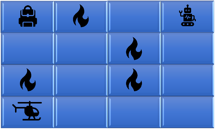
(a) (b)
Definition 1 (Non-Markovian Reward Decision Process)
An NMRDP is a tuple , where is a finite set of states, is a distinguished initial state, is a finite set of actions, is a probabilistic transition function, is an alphabet (i.e. the power set of a set of atomic propositions ), is a labeling function, and is a non-Markovian reward function.
The labeling function maps states of the NMRDP to the alphabet that defines the language of the underlying objective. This alphabet denotes semantically meaningful events observed in given states. Given a sequence of states , the corresponding trace is given by . Given positive and negative examples of such traces, the proposed non-Markovian IRL solution can learn the underlying LTL formula that captures the objective of the agent.
Given an NMRDP, the objective of reinforcement learning (RL) is to learn an optimal policy , where denotes the space of probability distributions over the action space . An optimal policy is one that maximizes the expected reward observed by the agent, as given by Equation (1), where is an arbitrary sequence of states sampled based on the enacted policy and is a discount factor.
| (1) |
The objective is to learn a reward signal that best characterizes the given observations of behavior from an expert. For a given process, the performance of the learned reward can be measured in terms of the inverse learning error (ILE) given by [19], where denotes the value function computed using the optimal policy from the true reward signal and denotes the same for the policy derived from the reward signal learned using IRL. the value functions are computed over the NMRDP by leveraging the learned policy using the true reward function (the one defined by ). A learned reward signal is said to generalize if the ILE is low when compared to the ground truth.
Consider the RL problem illustrated in Figure 1(a). The NMRDP that defines this problem is given by , where consists of sixteen states as denoted by the grid position of the agent, with starting state (top right, at position ()). The action space is given by the cardinal directions with the obvious deterministic transition dynamics . The labeling function is given by }, , and . Suppose that the objective of the agent is to eventually obtain the cargo and, once the cargo is obtained, the agent must avoid the dangerous areas and eventually reach the rendezvous point. This is given by the LTL formula . In the IRL context, this objective is not known to the agent directly and it must instead learn from expert demonstrations.
Our proposed approach enables the use of both positive and negative traces of behavior to guide the learning process. In this example, a positive trace can be since it clearly satisfies the underlying objective given by . A bad trace can be as generated by the policy of moving left three times and then down three times. Since trajectories of states given by the expert (or produced by the expert policy) have a corresponding trace induced by the labeling function , we assume that the traces are given over the alphabet as opposed to the state space of the NMRDP.
3 Preliminaries
Propositional Logic. Let Var be a set of propositional variables, which take values from ( interpreted as and as ). The set of formulae in propositional logic — with formulae denoted herein as Greek letters — is defined inductively as follows:
We use the usual syntactic sugar , , and .
A propositional valuation is defined as a mapping , which maps propositional variables to Boolean values. The semantics of this logic, given by the satisfaction relation , are defined inductively as: (1) iff ; (2) iff ; (3) iff and . If we say models . A formula is said to be satisfiable if there exists a model for it. There are practical tools, called SAT solvers, that can check satisfiability of the formulae.
An alphabet is a non-empty, finite set of symbols. A finite word over is a finite sequence of symbols from . The empty sequence is called the empty word, denoted . The domain of , denoted is the set of positions in . Thus, and . The length of a finite word is denoted , with . The set of all finite words over is denoted . An infinite word over is an infinite sequence of symbols with . The set of all infinite words over is denoted .
Given a finite word , we write for the symbol at position . The subsequence of from index to index , both inclusive, is denoted as , while denotes the suffix of starting from index . When clear from context, we write for .
Linear Temporal Logic (LTL). Let be a set of propositional variables. LTL [20] is an extension of propositional logic with temporal modalities, which allows the expression of temporal properties. Formulae in LTL are defined inductively. An LTL formula over is defined by the following grammar:
Using the above, the formulae and can be derived. The size of an LTL formula denoted by is the number of subformulae in it. For example, if , then . We say that an infinite word satisfies an LTL formula , and we write , if:
- •
- •
- •
- •
- •
.
The language of an LTL formula is defined as
Two LTL formulae having the same language are called equivalent. In this paper, we learn formulae that are in the GF-fragment of LTL, where only the G and F modalities are allowed apart from Boolean connectives. Since the LTL formulae can be converted into negation normal form (NNF), we learn formulae only in NNF. Given an LTL formula , the syntax tree of is a tree labeled with variables, Boolean connectives and temporal modalities. The variables always appear at the leaf nodes, while temporal modalities and Boolean connectives are internal nodes. For example, we present the syntax tree of the formula in Figure 1(b). The depth of an LTL formula is the maximum of distances of the root to leaves in the corresponding syntax tree. The depth in Figure 1(b) is 3. Although, LTL is defined over infinite words, we observe only finite executions of the systems. Therefore, we defined samples with finite words as follows.
Samples. A sample is a pair of two finite, disjoint sets . The words in are positive traces while words in are negative traces. For an LTL formula , we say iff and . We learn an LTL formula from a given sample.
4 Occam’s Razor for LTL
Given an LTL formula and a finite word , we design a valuation function that quantifies the parsimony of in explaining . Intuitively, a pair scores high if all of the subformulae of the formula contribute in accepting in . However, we do so in a nuanced fashion by geometrically attenuating the effect of parsimony with the length of the word. For example, should score well along with word but should not do well with word , since the subformula did not contribute to the acceptance. Similarly, should score better along with word than .
4.1 Quantifying Expressive Parsimony
Let us present a valuation function first. Let represent the set of NNF GF-fragment formulae over . We interpret LTL formulae over finite words and define the quantitative semantics in terms of a valuation mapping , where . The valuation mapping is defined over a word inductively:
Here is a shorthand for . If , then is non-zero. This scheme is parameterized by two discount factors: the temporal discount factor and the nesting discount factor .
For the literals, we assign valuation zero or one if the word satisfies the literals or not. We interpret conjunction as multiplication, which implies we need both subformulae to do well on the word. We interpret disjunction as an addition, which implies we give a high score to the formula if any of the two subformulae does well on the word. Our interpretation of computes the discounted sum of the value of at each position of the word. To reduce the weight of a letter appearing further in the word, we apply the temporal discount of . Our interpretation of computes the discounted score of at the earliest position where has a non-zero score. We apply the nesting each time we construct a more complex formula, i.e. we go deeper in the nested structure of the LTL formula. The discount values and are parameters defined by the user to control nesting complexity and temporal complexity.
Example 1
Consider the formula for and the word . Then holds for the first time at the position , and for all , is not present in . Thus, , making . Note that our valuation assigns non-zero scores only for satisfiable formulas.
We extend the notion of a valuation from a word to a sample in a natural fashion. For a sample , the valuation of is taken as the sum of valuations over all positive traces in the sample:
This scheme attempts to match intuition about the operators. We posit that while the definition of the valuation functions is subjective, natural variations do not provide any significant theoretical advantages to our paradigm. For example, One may assign as the minimum of and [21]. This valuation ensures that both and must score high for to score high. However, the function is not sensitive to the formula that has a higher value. Therefore, the learning algorithm becomes unguided for one part of the formula. This suggests a modification to the valuation function that takes both the subformulae into account symmetrically, without flattening one of the subformulae. Our valuation function for the conjunction of two formulae, defined as their product is based on this idea.
5 Learning Algorithms
As our main contribution, we propose learning algorithms to solve the following problem. Given a sample =(P,N) over finite words, compute an LTL formula in the GF-fragment that best describes and is consistent with . That is, has the highest score, based on the valuation described above, among all formulae such that for all , and for all , .
To achieve the goal of ranking formulae based on a quantitative notion of satisfiability, we propose the techniques of Constraint System Optimization (Section 5.1) Optimized Pattern Matching (Section 5.2) and Hybrid Pattern Matching (Section 5.3). In the first one, we get a sample and a depth as input. We encode the syntax tree of this unknown formula of depth along with constraints to compute the score of each node in the tree. The second one makes use of a formula template pattern provided by the user, but has unknown propositional variables. We encode constraints which allow mapping these variables to unique variables occurring in the sample. The third one is a “hybrid” approach, a middle ground incorporating both of the above techniques. We use an optimizing SMT solver to solve the constraints to find the best formula for the sample with the highest score according to the valuation function.
5.1 Constraint System Optimization
In Algorithm 1, we present the method to compute the optimal formula with the highest score for a sample along with the desired depth of the formula. This is obtained by computing and optimizing the scores of a class of formulae of depth , constrained to be well formed and to be satisfied by . We reduce the construction of an LTL formula for a sample to a constraint system , which is constructed in three parts as:
| (2) |
The first part encodes the structure of a syntax tree (ST) representing an unknown formula, while the second and third encode the functional constraints on the score of each node enforced by the operators that make up the formula.
To encode the formula structure, we use a syntax tree with identifiers for the set of nodes, where . We assume herein that the root node is identified as . We have the child relations and , such that (or ) iff the node is the left (right) child of node . The only child of unary operators is considered as a left child by assumption. For each node and possible label , we introduce a Boolean variable indicating whether the node is labelled with an operator () or variable (). The formula is constructed as the conjunction of formulae (3) through (11).
| (3) | |||||
| (4) |
The constraint given by expression (3) ensures the two properties that each node must accept at least one label, and that it must accept at most one label, while expression (4) ensures that the leaf nodes are labelled with propositional variables, and not operators (since they have no children).
Next, we encode the functional constraints imposed by the operators. For this, to each node , we attach a set of real variables representing its score at each point in a trace , where is defined below. For a given trace we construct as the conjunction of:
| (5) | |||
| (6) | |||
| (7) |
| (8) | |||
| (9) | |||
| (10) | |||
| (11) |
Corresponding to Boolean variables and to each operator, the constraints encode the calculation of the valuation of a given node as a function of the valuation of its children, as defined in Section 4. The score for a node labelled G at a position in the trace is described by the constraint (10). The first conjunct encodes the actual score as a function of its child, adding the child’s score over all positions in the input word, scaled by an exponential. The second conjunct simply ensures that the G-property holds in a classical sense, i.e., that its child has positive valuation at all positions. Similarly, F is encoded in constraint (11), where we look for the first position where its child has positive valuation. The score of its child is exponentially scaled so as to diminish the contribution from an occurrence far away from the start.
Finally, we optimize the score of the syntax tree using the score of the root node w.r.t. the constraint system ( Algorithm 1). Then we use the resulting model to label the tree, obtaining the optimal formula of chosen depth. By iterating over , we may obtain the minimal such formula. Next, we establish the correctness and soundness of this algorithm.
Lemma 1 (Well-Formedness)
The proof is a straight forward argument. In one direction, the constraints ensure that the forms a well formed binary tree. The encoding requires matching this binary tree with the parse tree of the given formula. In the converse direction, one can recursively construct the parse tree of a formula which satisfies the constraint system.
Theorem 5.1 (Completeness)
Given a sample , if there exists an LTL formula of depth such that , then there exists a model satisfying the constraint system (2 - 11), i.e. such that the parse tree encodes the formula and for each node and position in each trace , , where is the formula encoded by the subtree with root at node .
Proof
We induct on the depth of the formula.
Base case:
for some propositional variable , and .
Setting in and resolving the constraints, for each positive trace we are left with
| (12) | |||
| (13) |
Constraint 13 encodes the valuation function . We assign the same value to it in .
Since for each positive trace , we have , and hence, , and the constraint system is satisfied.
Similarly for negative traces, constraint 12 changes to , and since , we have , and the constraint system is satisfied.
Induction: Given the system is complete for all depths , we show it is complete for depth .
We prove this for each top-level operator:
Assuming — since , for each positive trace , we must have atleast one of and , and for each negative trace , we have .
Construct new samples and with containing the positive traces which satisfies, and for . By the induction hypothesis, we can find satisfying models for the constraint systems and , say and .
Using these, we construct a satisfying model for , . Assign to the the syntax tree encoding for . Through , the values of are known over . Without loss of generality, set the unknown values (over ) to 0. Similarly for and .
The constraint system for positive traces reduces again to
| (14) | |||
| (15) |
where nodes are the root node and its left and right children respectively. The models and ensure that both the terms on the RHS for are non-negative, and for each trace, atleast one is positive. Assigning the respective values to in , since the sum of a non-negative and a positive value is greater than 0, the system is satisfied.
For negative traces, we require . Clearly, the models of the subformulae ensure that both terms on the RHS for are zero. Hence, their sum is zero as well. Hence, the negative trace constraints are also satisfied under this .
is the required model.
Assuming — we must have , and for each negative trace , we have atleast one of and .
The proof proceeds identically to the previous case, except with a partitioning of the negative traces. Similar to the sum-based constraint system for , we have the product-based system for positive traces with the same notation as before
| (16) | |||
| (17) |
Again, the models of the subformulae ensure that both terms on the RHS for are positive, hence so is their product.
For negative traces, without loss of generality we assign to the unknown values over the complements . We have
| (18) | |||
| (19) |
and the models ensure atleast one of the terms in the RHS for is zero, and hence so is the product.
The constraint system is satisfied, and is the required model.
Assuming — we must have satisfied at every point on every positive trace and to not be satisfied on some point on each negative trace, i.e.
| (20) | |||
| (21) | |||
| (22) |
By taking all possible suffixes of traces in , construct , and by resolving the existential quantifier, collect relevant (non-satisfying) suffixes of as . Generate the new sample .
By construction, . Using the induction hypothesis, there exists a model satisfying the constraint system . We use to construct a model for .
Setting the values for as encoding , we are left with the reduced constraint system
| (23) |
| (25) |
For positive traces, from , we have an assignment for each of the terms in the sum for being positive (we posed them as positive traces in ). Hence, their sum is positive too, and adding these inferred assignments for , the constraints are satisfied.
For the negative traces, adding the assignments from , clearly the constraints cannot be satisfied for each parameter in the sum for , by construction. Thus, .
is the required model.
Assuming — the proof proceeds identically to the previous case, with existential quantification in the positive case, and suffix construction in the negative, since these are dual operators.
The induction is complete.
Theorem 5.2 (Soundness)
Proof
We induct on the depth parameter of the constraint system.
Base case: d = 0.
Since there is only a single leaf node, the model must have one of the propositional variable mapped to it, say . With this, the constraint system reduces to
| (26) | |||
| (27) |
Clearly, due to the constraints, for each trace . In particular, for , and with the constraints, we must have , which, by the LTL semantics implies .
Similarly for negative traces we find .
Combining these, we have , and hence is the required LTL formula of depth 0.
Induction: Given the system is sound for all depths , we show it is sound for depth .
We prove this for each top-level operator in the constraint encoding:
The top-level operator is obtained by checking which of holds under . The constraint system ensures there is exactly one. We assume the have been processed to obtain the encoded formula, say .
Our task is now to show that .
Assuming — We have the reduced constraints
| (28) | |||
| (29) |
For positive traces, in particular the constraints on the root-node imply at least one of and must hold, where are the left and right children of the root-node 1 respectively. And for negative traces we have .
In conjunction with the rest of the constraints, this is precisely two copies of the constraint system .
In either case, i.e. for the left or right child being non-zero, the induction hypothesis implies that the subformula holds over the sample , i.e. (or ). And since this is a subformula of , by introduction of , .
Assuming — Proof proceeds similar to the previous case, with a case-bifurcation in the negative traces instead of the positive ones.
Assuming — Again, we have the reduced constraint system
| (30) |
| (31) |
First, in the case of the positive traces, since , we must have the first clause of the score constraint holding (since the second clause evaluates to false). Thus, for each point in the trace, we must have with notation as before.
For negative traces, we can reduce the constraints on further to obtain
| (32) |
implying there exists a position for which .
As before, taking all possible suffixes of traces in , construct , and by resolving the existential quantifier above, collect relevant (non-satisfying) suffixes of as . Generate the new sample . Combined with the constraints above, we have a satisfying assignment to by restricting as needed to the smaller system.
Thus, by the induction hypothesis, for each trace , holds on every suffix of . By the semantics of the operator G, we have .
Further, for each negative trace , does not hold on some suffix of . Again, by the semantics of G, .
Thus, as required.
Assuming — Proof proceeds similar to the previous case, with existential quantification on the positive traces instead of the negative.
The induction is complete.
Corollary 1 (Valuation Equivalence)
The valuation semantics are equivalent to the LTL semantics. For any LTL formula and trace , iff .
Proof
Forward Direction :
Given an LTL formula and trace such that , we can construct a satisfying assignment to the constraint system by Theorem 5.1 where and is the depth of . Further, the theorem guarantees . This is the required condition.
Backward Direction :
Given an LTL formula and trace such that , construct the constraint system as before. Iteratively assign to each the value , where is the subformula at node in the parse tree. After assignment with constraints, as given, satisfying the constraint. By Theorem 5.2, as required.
5.2 Optimized Pattern Matching
We now present a variation of Algorithm 1 where the input consists of a sample along with a user-provided formula pattern, where the propositional variables are unknown. This approach is in the spirit of [22], where a formula template is used instead of just a depth as in Algorithm 1. We generate a static syntax tree by parsing the given pattern, with pattern propositional variables becoming the leaves. In addition to the constraints discussed in Section 1, constraint (33) ensures the mapping of the pattern variables to exactly one variable in the given sample, where represents the set of variables in the given pattern and stands for the mapping of pattern variable to the sample variable .
| (33) |
The constraint (33) specifies that each pattern variable is mapped to a sample variable, and no pattern variable is mapped to two sample variables. For an example of how this approach and the one defined in the previous subsection is combined into a hybrid approach, which is presented as follow.
5.3 Hybrid Pattern Matching
The algorithms defined in sections 5.1 and 5.2 suffer from a common drawback, though at different ends of the spectrum. In the first, we work with increasing depth to find the optimal formula and constraint sizes may grow quickly as a result. In the second, we start with a formula template and many formulae are not considered since we are guided by the template pattern. This makes this approach insufficiently expressive in comparison with constrained system optimization.
To remedy this, we introduce a middle ground, where, instead of attempting to learn formulae from scratch or from explicit patterns, we learn subformulae within some pattern. A subformulae argument with being a prescribed maximum depth for the subtree is provided as part of the pattern, parsed into the tree as an abstracted empty formula with constraints constructed for the specified nodes explicitly, and for the subformulae recursively in the manner as described in Algorithm 3. In Figure 2, we show an example of the hybrid pattern , where is an unknown formula of depth and is an unknown proposition.
5.4 Compositional Ranking
We describe an alternative greedy search for optimal formula, which bypasses constraint solving and optimizations, by pruning the search space of formulae. We begin by enumerating all formulae of depth zero, i.e., all literals in our system as obtained after parsing input traces. We consider all compositions of these literals with the operators present. After enumerating the literals, we perform an “F-check” : for any , the F-check tests whether, in any input sample, holds. If a formula passes an F-check, it is retained to produce formulae of higher depth, else it is removed (Algorithm 2). We have implemented more custom options to prioritise certain parts of the search space (Section 5.5).
5.5 Prioritize Variables.
Finally, we have added one more heuristic in our implementation. In case there is a large set of events and we want to bias the focus of our search towards certain letters in the traces that do not occur very often, we may adjust the value assigned to each propositional variable . In our default scheme, we assign if contains . A user may assign a value greater than to variables that are desirable and assign less than for the variables that are not. This allows for mining specifications pertaining to the prioritized variables in cases where several competing well ranked specifications are present. Let be the map from the propositional variables to their priority. We replace equation (6) by the following formula where we return score instead of .
| (34) |
In the Dining Philosophers problem (see Section 6.4), we may wish to verify individually whether the properties are being satisfied for a single philosopher (thread). By giving a higher weight to the properties of this philosopher, we can guide the tool to learn the relevant properties and verify them. This can be expanded to studying specific applications or threads in varied noisy data where the target of interest is either known apriori or is inferred from preliminary unguided results.
The suggested variations and their results indicate that our method is viable to be adapted to an application at hand, where we want to bias our ranking to give preference to a desired class of formulae.
6 Experiments
We have implemented the preceding algorithms in a tool called QuantLearn. In this section, we present the results of QuantLearn on a set of traces sampled from a grid-world environment running under OpenAI Gym. QuantLearn is implemented in C++. For the optimization, it takes a set of positive traces, a (possibly empty) set of negative traces, and a formula template (which can simply be , a search depth of with no specification) or a combination, while the compositional ranking takes as input the traces along with a maximum search depth. Our implementation uses SMT solver Z3 [18] for the optimizations. All our queries to Z3 are quantifier-free. For optimization, QuantLearn returns a formula with maximal score according to our scheme, while for compositional ranking, it returns a list of all satisfying formulae in the search space, sorted by score. In our experiments, we used a discount factor and also used to decay each time we build deeper formulae in order to bias the ranking towards simpler formulae. We evaluated the performance of QuantLearn on a 64-bit Linux system with an AMD Renoir Ryzen 5 (4500U) laptop CPU. We set seconds as timeout. We compare with Texada[23] and the SAT based tool Traces2LTL [24].
Due to the vastly different mechanisms of the tools and algorithms in contention, an apples-to-apples comparison is impossible. The compositional ranking input accepts no pattern input, constraint system optimization accepts none to partial input, while Texada requires complete template specification as input, and does not utilize negative trace samples either. We defer the comparison with Traces2LTL to a later point in the section, as it accepts a different method of trace input, i.e., rational traces. As a whole, QuantLearn is capable of reliably extracting properties from limited, noisy data, and with the addition of compositional ranking, is able to match the performance of existing tools while requiring no guidance for inference. The results are summarized in Figure 3.
When comparing to Traces2LTL, since both it and our constraint system optimization encode a similar system, the former restricted to just boolean variables instead of real scores, for large trace inputs as tested above, both output similar results, and due to avoiding searching real parameters, Traces2LTL outperforms QuantLearn. For smaller noisy traces, with effective number of trace events ranging approximately from 20 to 500, Traces2LTL outputs several possible formulae, most containing the extraneous noisy variables, since it relies on Z3 to present the formulae in arbitrary orders as satisfying assignments. In this scenario, QuantLearn reliably bypasses noise and extracts formulae of up to depth 3 reliably, and we suggest this as the ideal use-case for constraint system optimization over other algorithms.
Traces2LTL [24] also presents an alternate method of using decision-tree learning to remedy scalability issues of SMT solver based systems for larger inputs. However, compositional ranking is several orders of magnitude faster than either of the two methods for higher depth formulae while producing more succinct specifications, and is thus suggested as an alternative in that case.
Due to the different natures of inputs for the programs, we split the tests to compare against each. We compare performance with the simpler Texada and reliability against the expressive Traces2LTL.
For the NMRDP tests with Traces2LTL, given the input, it was asked to iteratively produce 5 satisfying assignments, and the ILE was averaged over these results, since the tool does not have a preferential ordering scheme. In several cases, the correct generator was one of the 5 assignments presented, which scored an ILE of 0, while the others, depending on compatibility with the sample and closeness to original, were spread between an ILE of 0.3 and 0.8 for randomized grids.
For QuantLearn, with both algorithms, one of the formulas was learnt as a close alternative (different for both algorithms too!), leading to an increased ILE of 0.25-0.35 in that case, while the other formulas were learnt exactly. The results were averaged over runs and formulas for all three.
Traces2LTL was considered for these tests over Texada to maintain a level playing field regarding guidance. Since for Texada, to obtain the correct formula, one must know and provide the entire template.
Due to scalability issues of the SAT/SMT based methods, both Traces2LTL and QuantLearn with constraint optimization were provided a randomly chosen subset of the generated traces, while QuantLearn with compositional ranking processed the entire set.
| Constraint | Comp. | Traces2LTL | |
| Optimization | Ranking | ||
| Mean ILE | 0.031 | 0.037 | 0.112 |
| Input size |
We consider two synthetic tests. First, we systematically generate trace of different sizes to compare performance and expressiveness of the different methods. After generating uniformly random traces, we add noise to each point in the trace in the form of two extraneous propositional variables with probability each. For these experiments, we maintained . We consider LTL formulae encoding some popular requirements.
6.1 Non-Markovian IRL
We apply learning techniques to generate a reward function over an MDP defined as a grid world to obtain an NMRDP, similar to the example in Figure 1(a). After generating a randomized grid environment labeled with propositional variables, we uniformly sample the grid taking actions compatible with an input automaton. This ensures that the generated traces satisfy a given formula. We use the same LTL properties as the previous case. We allow the MDP to randomly simulate for at least 100 steps, after which we wait for it to reach an accepting state. Through this method, we generated traces of length varying between 100 and 150, with 1000 positive and 1000 negative traces for each formula, amounting to a total trace length of at least across all positive and negative inputs. However, for constraint system optimization and Traces2LTL [24], due to timeouts, a smaller subset was randomly selected from the traces.
For our experiments, given an NMRDP in the form of a gridworld, we can compute the optimal policy using the preceding equation for three different DRA(Definition 2 in Section 6.3) objectives by computing three product MDPs. The first DRA objective is what we are trying to learn. We will denote the optimal policy here as computed on , where is the DRA representation of the LTL objective we are trying to learn. Then, we have the policy computed on , where is the DRA learnt using QuantLearn. Finally, we have the policy computed on , where is the DRA learnt using Traces2LTL [24]. We will take these three policies to generate our results in the form of the inverse learning error (ILE). We compute these value functions using uniformly random sampling of trajectories from every state in the NMRDP. We can then take a simple ratio (MeanILE in Table below) of the number of trajectories satisfied by , and divide it with the total number of trajectories, and report an average over multiple runs and inputs. In particular, we will compute two ILE values, comparing and . Our experiments demonstrate that the former is smaller than the latter, thereby providing evidence that our approach generalizes better for non-Markovian IRL than a competing one adapted to the IRL.
6.2 Runtimes with optimization for scores
We report the average runtimes for our approach with and without compositional ranking and compare it to that of Texada. In Figure 3a, we show the runtimes with different patterns of user specification over the different lengths of traces for constraint system optimization and optimized pattern matching. In Figure 3b we show runtimes for synthetic traces generated from the following common formulae with compositional ranking [24, 25].
| Property | Formulae |
|---|---|
| Absence | , |
| Response | , |
| Existence | , |
| Universality | , |
The length of the individual traces varies from 5 to 10,000. In Figure 3c we show runtimes for the generated traces with Texada. The comparison with Texada is difficult because it requires the complete formula template as input while we do not. The tests are thus performed with complete formula template as input, with which Texada outputs a list of possible formulae with propositions substituted in. In our eperiments, we found that Texada and compositional ranking perform comparably despite the fact that our approach requires no pattern input.
6.3 Non-Markovian Rewards and Product Construction
Since the non-Markovian nature of the reward signal in our setting can be represented by a regular or -regular language, we translate the problem of finding an optimal policy to one of finding a Markovian optimal policy over an augmented decision process by taking into account the structure of the regular language. Since we are learning LTL formulae, the corresponding structures are deterministic Rabin automata, though other choices of automata are possible.
Definition 2 (Deterministic Rabin Automaton (DRA))
A DRA is a tuple , where is a finite alphabet, is a finite set of states, is the initial state, is the transition function, and is the Rabin condition.
By taking the DRA representation of a regular reward signal and the underlying NMRDP, a product Markov Decision Process (MDP) can be computed. In particular, the reward signal of the MDP is defined only over the current state and action, thereby enabling the adoption of conventional Markovian solutions, such as value iteration. In order to define a reward signal for the product MDP, we must ensure that, when the acceptance condition of the underlying DRA is satisfied, the agent is rewarded. For this, we must compute maximal sub-MDPs known as maximal end components (MECs). Formally, for a DRA with acceptance condition , a MEC of the product MDP is accepting if and for some . The reward signal of the product MDP is defined whenever states with labels in are entered.
Definition 3 (Product LMDP)
Given NMRDP , DRA , the product LMDP is the tuple , where ; equals if and is otherwise; and if for some and is otherwise.
For a product LMDP , Equation (1) reduces to the equation below, where .
Since we are now reasoning about a Markovian reward over the product, the optimal value for a state can be computed using value iteration. In particular, we can initialize for all for some and for all . We can then iteratively refine these value functions by applying the following equation until convergence, where .
These equations converge to for all . The optimal policy can then be extracted as
6.4 Mining Formulae from the traces of Dining Philosophers
The dining philosophers problem [26] is a widely used example of a control problem in distributed systems and has become an important benchmark for testing expressiveness of concurrent languages and resource allocation strategies. We consider the problem with five philosophers p1, p2, p3, p4, p5 sitting at a round table. They are being served food, with a fork placed between each pair. Each philosopher proceeds to think till they are hungry, after which they attempt to pick up the forks on both of their sides, eating till they are full, but only when forks on both sides are available. After they are done eating, they put the forks down back on to either of their sides, and continue thinking. The goal is to establish lockout-freedom, i.e., each hungry philosopher is eventually able to eat. We use QuantLearn to mine LTL formulae from a trace of size 250 from Texada tests [23]. We searched several mined properties using different templates presented in Figure 4.
- •
When we gave the pattern (invariant, depth 1) to QuantLearn and required it to learn a property, we obtained the property GFp1 is thinking. The mined property acts as a verification of the liveness of the system. QuantLearn took 12 seconds to find the property. While this provides a general fact about the system, building upon this result, we can guide the tool to find more relevant properties for higher depths.
- •
When we gave the pattern to QuantLearn and required it to learn a property, we obtained the property . The mined property illustrates that adjacent philosophers cannot acquire forks at the same time, ensuring that our lock, the availability of forks does indeed prevent philosophers from eating. QuantLearn took 72 seconds to find the property.
- •
When we gave the pattern to QuantLearn and required it to learn a property, we obtained . This property is a richer demonstration of deadlock freedom for philosopher 1, ensuring that they both enter and exit their critical section, i.e., the eating state. QuantLearn took 165 seconds to find the property.
by observing their runs. Using patterns, QuantLearn can be guided to learn properties of specific interest.
| Input | Output | Interpretation |
|---|---|---|
| GFp1 is thinking | Liveness property | |
| Mutual exclusion | ||
| Deadlock freedom | ||
7 Related Work
[27] present a detailed landscape of the algorithms, challenges, and the state-of-the-art in IRL. [2] formalized the first computation solution to IRL based on linear programming to demonstrate the effectiveness of IRL. Among more recent efforts, IRL is solved using techniques from entropy optimization[28, 29, 30], maximum likelihood estimation [31, 32], and reformulating the problem as a classification task [33]. These techniques have shown much promise and have been applied successfully to problems such as maneuvering remote-controlled helicopters [34] and Atari games [35].
Grammatical inference is a related area [36] concerned with learning grammars and their automata representations [37, 38]. Active techniques rely on querying the system under learning to guide the inference process, whereas passive grammatical inference leverages a static set of trace behavior without making further queries for additional data. The former is exemplified by algorithm [39], whereas the latter generally relies on state-merging procedures and can be used to learn probabilistic automata [40], MDPs in the context of model checking [41], timed automata [42], and regular decision processes [43]. There is a growing literature on the application of grammatical inference to RL. This typically entails the learning of weighted DFAs, known as reward machines [44, 45, 46].
However, the application of grammatical inference for IRL has not been explored. Indeed, the foregoing RL methods learn automata from traces of the underlying decision process with a given reward signal, not from traces of an expert policy over unknown and unobservable environment. The problem of learning LTL formulae from traces is a form of grammatical inference that has been well-studied. Two of the methods most related to our own are presented in [22] and [24]. The focus of [24] is to produce the minimal formula which is consistent with a rational sample represented as a lasso. The problem of matching formulae with traces is encoded as a constraint system and a satisfying assignment yields the learned property. However, requiring the inputs to be lassos significantly restricts the application to real scenarios. The method in [22] requires a user-defined input template of the LTL formula which they would like to satisfy and outputs all possible propositional substitutions consistent with the sample.
We seek to combine some of these ideas and try to eliminate their restrictions with a method that may be used on finite traces obtained from real systems, and output results relevant to the user. To allow the algorithms to quantitatively distinguish formulae, we supplement them with the idea of a ranking scheme as a parameter to the methods. Our ranking scheme quantitatively scores each formula against a finite word. It expands on intuitive ideas used to formulate distances in regular language spaces [47, 48]. The suggested scheme assigns a formula a high score if it expresses most features of the word. A formula can score well on a word if it provides longer evidence of validity with respect to larger parts of the word. For example, will score more on the word than on the word , since it contains more evidence for the word to have been a prefix of . Furthermore, our suggested scoring scheme encourages simpler formulae over complex ones in equivalence classes; that is, from an equivalence class of LTL formulae, the ones with smaller parse trees will be preferred.
The papers closest to our work are [22] and [24]. The focus of [24] is to produce the minimal formula which is consistent with a rational sample irrespective of the expressiveness, while [22] requires a user defined input template of the LTL formula which they would like to satisfy. Both work with infinite traces: [24] takes rational traces in the form where are typically words of length , while [22] mines specifications from finite traces, and appends them with an infinite sequence of terminal events. [49] considers finite traces, and develops a LTL checker which takes an event log and a LTL property and verifies if the observed behaviour matches some bad behaviour. The papers [50, 51] look at the application of monitoring the execution of Java programs, and check LTL formulae on finite traces of these programs. In [52], the authors focus on mining quantified temporal rules which help in establishing data flow analysis between variables in a program, while in [53] software bugs are exposed using a mining algorithm, especially for control flow paths. [54] looks at process mining in the context of workflow management. The tool PISA [55] is developed to extract the performance matrix from workflow logs, while a declarative language is developed to formulate workflow-log properties in [56]. Tool Synoptic [57] on the other hand, follows a different approach and takes event logs and regular expressions as input and produces a model that satisfies a temporal invariant which has been mined from the trace.
8 Conclusion and Future work
In this paper, we presented a novel scheme to quantitatively evaluate LTL formulae. Our evaluation schema is designed such that the score received by a word is proportional to how well it represents the formula. Thus, words which are “good representatives” score higher than words which merely satisfy the formula (and hence qualify to be “poor representatives”).
One of our contributions is to use this schema to mine LTL formulae from the traces of reactive systems. Our approach presents a viable solution to non-Markovian inverse reinforcement learning (IRL) in settings where the reward signal can be captured as LTL formulae. A possible direction for future work is to enhance our optimizer so that it works seamlessly with a broad spectrum of constraints.
References
- [1] Stuart Russell. Learning agents for uncertain environments. In Proceedings of the eleventh annual conference on Computational learning theory, pages 101–103, 1998.
- [2] Andrew Y Ng and Stuart Russell. Algorithms for inverse reinforcement learning. In Icml, volume 1, page 2, 2000.
- [3] David Abel, Will Dabney, Anna Harutyunyan, Mark K Ho, Michael Littman, Doina Precup, and Satinder Singh. On the expressivity of markov reward. Advances in Neural Information Processing Systems, 34, 2021.
- [4] Rodrigo Toro Icarte, Toryn Klassen, Richard Valenzano, and Sheila McIlraith. Using reward machines for high-level task specification and decomposition in reinforcement learning. In International Conference on Machine Learning, pages 2107–2116. PMLR, 2018.
- [5] Amir Pnueli. The temporal logic of programs. In 18th Annual Symposium on Foundations of Computer Science (sfcs 1977), pages 46–57. IEEE, 1977.
- [6] Christel Baier and Joost-Pieter Katoen. Principles of Model Checking (Representation and Mind Series). The MIT Press, 2008.
- [7] Paul Gastin and Denis Oddoux. Fast ltl to büchi automata translation. In International Conference on Computer Aided Verification, pages 53–65. Springer, 2001.
- [8] Ronen I Brafman and Giuseppe De Giacomo. Planning for ltlf/ldlf goals in non-markovian fully observable nondeterministic domains. In IJCAI, pages 1602–1608, 2019.
- [9] Giuseppe De Giacomo and Moshe Y Vardi. Linear temporal logic and linear dynamic logic on finite traces. In IJCAI’13 Proceedings of the Twenty-Third international joint conference on Artificial Intelligence, pages 854–860. Association for Computing Machinery, 2013.
- [10] E. M. Hahn, M. Perez, S. Schewe, F. Somenzi, A. Trivedi, and D. Wojtczak. Omega-regular objectives in model-free reinforcement learning. In TACAS 2019, Proceedings, Part I, volume 11427 of LNCS, pages 395–412. Springer, 2019.
- [11] A. K. Bozkurt, Y. Wang, M. M. Zavlanos, and M. Pajic. Control synthesis from linear temporal logic specifications using model-free reinforcement learning. In ICRA, pages 10349–10355. IEEE, 2020.
- [12] D. Sadigh, E. S. Kim, S. Coogan, S. S. Sastry, and S. A. Seshia. A learning based approach to control synthesis of Markov decision processes for linear temporal logic specifications. In CDC, pages 1091–1096, 2014.
- [13] Alberto Camacho, Rodrigo Toro Icarte, Toryn Q Klassen, Richard Anthony Valenzano, and Sheila A McIlraith. Ltl and beyond: Formal languages for reward function specification in reinforcement learning. In IJCAI, volume 19, pages 6065–6073, 2019.
- [14] Alper Kamil Bozkurt, Yu Wang, Michael M Zavlanos, and Miroslav Pajic. Control synthesis from linear temporal logic specifications using model-free reinforcement learning. In 2020 IEEE International Conference on Robotics and Automation (ICRA), pages 10349–10355. IEEE, 2020.
- [15] Ernst Moritz Hahn, Mateo Perez, Sven Schewe, Fabio Somenzi, Ashutosh Trivedi, and Dominik Wojtczak. Mungojerrie: Reinforcement learning of linear-time objectives. arXiv preprint arXiv:2106.09161, 2021.
- [16] Jan Kretínský and Javier Esparza. Deterministic automata for the (f, g)-fragment of LTL. In Computer Aided Verification - 24th International Conference, CAV 2012, Berkeley, CA, USA, July 7-13, 2012 Proceedings, pages 7–22, 2012.
- [17] Javier Esparza, Jan Kretínský, and Salomon Sickert. One theorem to rule them all: A unified translation of LTL into -automata. In LICS 2018, 2018.
- [18] Leonardo de Moura and Nikolaj Bjorner. Z3: An efficient smt solver. In TACAS, volume 4963 of LNCS, pages 337–340. Springer Berlin Heidelberg, 2008.
- [19] JD Choi and Kee-Eung Kim. Inverse reinforcement learning in partially observable environments. Journal of Machine Learning Research, 12:691–730, 2011.
- [20] Christel B and Joost-Pieter K. Principles of model checking. MIT Press, 2008.
- [21] Paulo Tabuada and Daniel Neider. Robust linear temporal logic. arXiv preprint arXiv:1510.08970, 2015.
- [22] Caroline Lemieux, Dennis Park, and Ivan Beschastnikh. General ltl specification mining (t). In 2015 30th IEEE/ACM International Conference on Automated Software Engineering (ASE), pages 81–92. IEEE, 2015.
- [23] Texada. https://github.com/ModelInference/texada, 2015.
- [24] D. Neider and I. Gavran. Learning linear temporal properties. In 2018 Formal Methods in Computer Aided Design (FMCAD), pages 1–10, 2018.
- [25] Matthew B Dwyer, George S Avrunin, and James C Corbett. Property specification patterns for finite-state verification. In Second workshop on FMSP, 1998.
- [26] Edsger W Dijkstra. Hierarchical ordering of sequential processes. In The origin of concurrent programming, pages 198–227. Springer, 1971.
- [27] Saurabh Arora and Prashant Doshi. A survey of inverse reinforcement learning: Challenges, methods and progress. Artificial Intelligence, 297:103500, 2021.
- [28] Brian D Ziebart, Andrew L Maas, J Andrew Bagnell, Anind K Dey, et al. Maximum entropy inverse reinforcement learning. In Aaai, volume 8, pages 1433–1438. Chicago, IL, USA, 2008.
- [29] Abdeslam Boularias, Jens Kober, and Jan Peters. Relative entropy inverse reinforcement learning. In Proceedings of the fourteenth international conference on artificial intelligence and statistics, pages 182–189. JMLR Workshop and Conference Proceedings, 2011.
- [30] Tuomas Haarnoja, Aurick Zhou, Pieter Abbeel, and Sergey Levine. Soft actor-critic: Off-policy maximum entropy deep reinforcement learning with a stochastic actor. In International conference on machine learning, pages 1861–1870. PMLR, 2018.
- [31] Monica C Vroman. Maximum likelihood inverse reinforcement learning. Rutgers The State University of New Jersey-New Brunswick, 2014.
- [32] Dexter RR Scobee and S Shankar Sastry. Maximum likelihood constraint inference for inverse reinforcement learning. arXiv preprint arXiv:1909.05477, 2019.
- [33] Edouard Klein, Matthieu Geist, Bilal Piot, and Olivier Pietquin. Inverse reinforcement learning through structured classification. Advances in neural information processing systems, 25, 2012.
- [34] Pieter Abbeel, Adam Coates, Morgan Quigley, and Andrew Y Ng. An application of reinforcement learning to aerobatic helicopter flight. Advances in neural information processing systems, 19:1, 2007.
- [35] Aaron Tucker, Adam Gleave, and Stuart Russell. Inverse reinforcement learning for video games. arXiv preprint arXiv:1810.10593, 2018.
- [36] Manuel Lopes, Francisco Melo, and Luis Montesano. Active learning for reward estimation in inverse reinforcement learning. In Joint European Conference on Machine Learning and Knowledge Discovery in Databases, pages 31–46. Springer, 2009.
- [37] James Jay Horning. A study of grammatical inference. Technical report, STANFORD UNIV CALIF DEPT OF COMPUTER SCIENCE, 1969.
- [38] Colin De la Higuera. Grammatical inference: learning automata and grammars. Cambridge University Press, 2010.
- [39] Dana Angluin. Learning regular sets from queries and counterexamples. Information and computation, 75(2):87–106, 1987.
- [40] Rafael C Carrasco and Jose Oncina. Learning stochastic regular grammars by means of a state merging method. In International Colloquium on Grammatical Inference, pages 139–152. Springer, 1994.
- [41] Hua Mao, Yingke Chen, Manfred Jaeger, Thomas Dyhre Nielsen, Kim Guldstrand Larsen, and Brian Nielsen. Learning markov decision processes for model checking. Electronic Proceedings in Theoretical Computer Science, 103:49–63, 2012.
- [42] Hua Mao, Yingke Chen, Manfred Jaeger, Thomas D Nielsen, Kim G Larsen, and Brian Nielsen. Learning deterministic probabilistic automata from a model checking perspective. Machine Learning, 105(2):255–299, 2016.
- [43] Eden Abadi and Ronen I. Brafman. Learning and solving regular decision processes. In Proceedings of the Twenty-Ninth International Joint Conference on Artificial Intelligence, IJCAI, pages 1948–1954. ijcai.org, 2020.
- [44] Rodrigo Toro Icarte, Ethan Waldie, Toryn Klassen, Rick Valenzano, Margarita Castro, and Sheila McIlraith. Learning reward machines for partially observable reinforcement learning. Advances in Neural Information Processing Systems, 32:15523–15534, 2019.
- [45] Zhe Xu, Ivan Gavran, Yousef Ahmad, Rupak Majumdar, Daniel Neider, Ufuk Topcu, and Bo Wu. Joint inference of reward machines and policies for reinforcement learning. In Proceedings of the International Conference on Automated Planning and Scheduling, volume 30, pages 590–598, 2020.
- [46] Zhe Xu, Bo Wu, Aditya Ojha, Daniel Neider, and Ufuk Topcu. Active finite reward automaton inference and reinforcement learning using queries and counterexamples. In Machine Learning and Knowledge Extraction - 5th IFIP TC 5, TC 12, WG 8.4, WG 8.9, WG 12.9 International Cross-Domain Conference, CD-MAKE 2021, Virtual Event, August 17-20, 2021, Proceedings, volume 12844 of Lecture Notes in Computer Science, pages 115–135. Springer, 2021.
- [47] Sean A Fulop and David Kephart. Topology of language classes. In Proceedings of the 14th Meeting on the Mathematics of Language (MoL 2015), pages 26–38, 2015.
- [48] Austin J Parker, Kelly B Yancey, and Matthew P Yancey. Regular language distance and entropy. arXiv preprint arXiv:1602.07715, 2016.
- [49] Wil M. P. van der Aalst, H. T. de Beer, and Boudewijn F. van Dongen. Process mining and verification of properties: An approach based on temporal logic. In ODBASE 2005.
- [50] K. Havelund and G. Rosu. Monitoring programs using rewriting. In ASE 2001.
- [51] K Havelund and G Roşu. Synthesizing monitors for safety properties. In TACAS, 2002.
- [52] David Lo, V-Prasad R, G R, and Kapil V. Mining quantified temporal rules: Formalism, algorithms, and evaluation. Science of Computer Programming, 2012.
- [53] Westley W and George C. Mining temporal specifications for error detection. In TACAS, 2005.
- [54] Rakesh A, Dimitrios G, and Frank L. Mining process models from workflow logs. In EDBT, 1998.
- [55] Michael Z M and Michael R. Workflow-based process monitoring and controlling-technical and organizational issues. In HICSS, 2000.
- [56] I. Beschastnikh, Y. Brun, J. Abrahamson, M. D. Ernst, and A. Krishnamurthy. Using declarative specification to improve the understanding, extensibility, and comparison of model-inference algorithms. IEEE Trans. Softw. Eng., 2015.
- [57] Ivan B, Yuriy B, Sigurd S, Michael S, and Michael D E. Leveraging existing instrumentation to automatically infer invariant-constrained models. In FSE, 2011.