Non-existence of negative curvesThanks: The second author was supported by a grant from the Simons Foundation (Award Number 710443) and by the UCR Academic Senate. The third author was supported by a NSERC Discovery grant.
Abstract.
Let be a projective toric surface of Picard number one blown up at a general point. We bring an infinite family of examples of such whose Kleiman-Mori cone of curves is not closed: there is no negative curve generating one of the two boundary rays of the cone. These examples are related to Nagata’s conjecture and rationality of Seshadri constants.
1. Introduction
Let be a projective toric surface defined by a rational triangle , and let be the blowup of at a general point . In this article we consider the question of whether the Kleiman-Mori cone of curves of is closed. The cone of curves of is two-dimensional, with one extremal ray generated by the class of the exceptional curve and the other extremal ray generated by a class of nonpositive self-intersection. If we can choose to be the class of an irreducible curve , we call this a negative curve of . In other words, a negative curve is any irreducible curve of nonpositive self-intersection, , different from . Our main result is to bring a family of examples of that have no negative curves, and hence their cones of curves are half-open.
Theorem 1.1.
Let be the triangle with vertices
where is a rational number in the interval , and let be defined over any algebraically closed field of characteristic . Then, contains no negative curve.
The set of varieties defined by a rational triangle contains as a subset all weighted projective planes . The examples in the theorem are not in this subset. However, any defined by a rational triangle is a quotient of by a finite abelian group.
Let us put this result in the context of [10]. In that article we considered all rational triangles and catalogued all known negative curves. Part of this work is summarized in Figure 1. We consider triangles with a horizontal base and the left and right edges with slopes and . Then, a triangle , or the blowup , corresponds to a point in the -plane. We may and will assume that is the identity point in the torus . A negative curve is defined by a Laurent polynomial that vanishes to order at the point and whose Newton polygon fits into a triangle of area . For each polynomial there may be many such triangles , hence the same polynomial can define a negative curve in many varieties . The set of all such for a fixed is a region in the -plane that typically has the shape of a diamond. In Figure 1, different diamonds correspond to different polynomials . If some contains a negative curve with strictly negative self-intersection, then this negative curve is unique in . This explains why the diamonds can intersect only at their boundary points, in which case contains two negative curves of zero self-intersection. Parts of the plane are not covered by any diamond. The varieties corresponding to these points are expected to contain no negative curve. The varieties in Theorem 1.1 correspond to points in the intersection of the diamonds labeled with and .
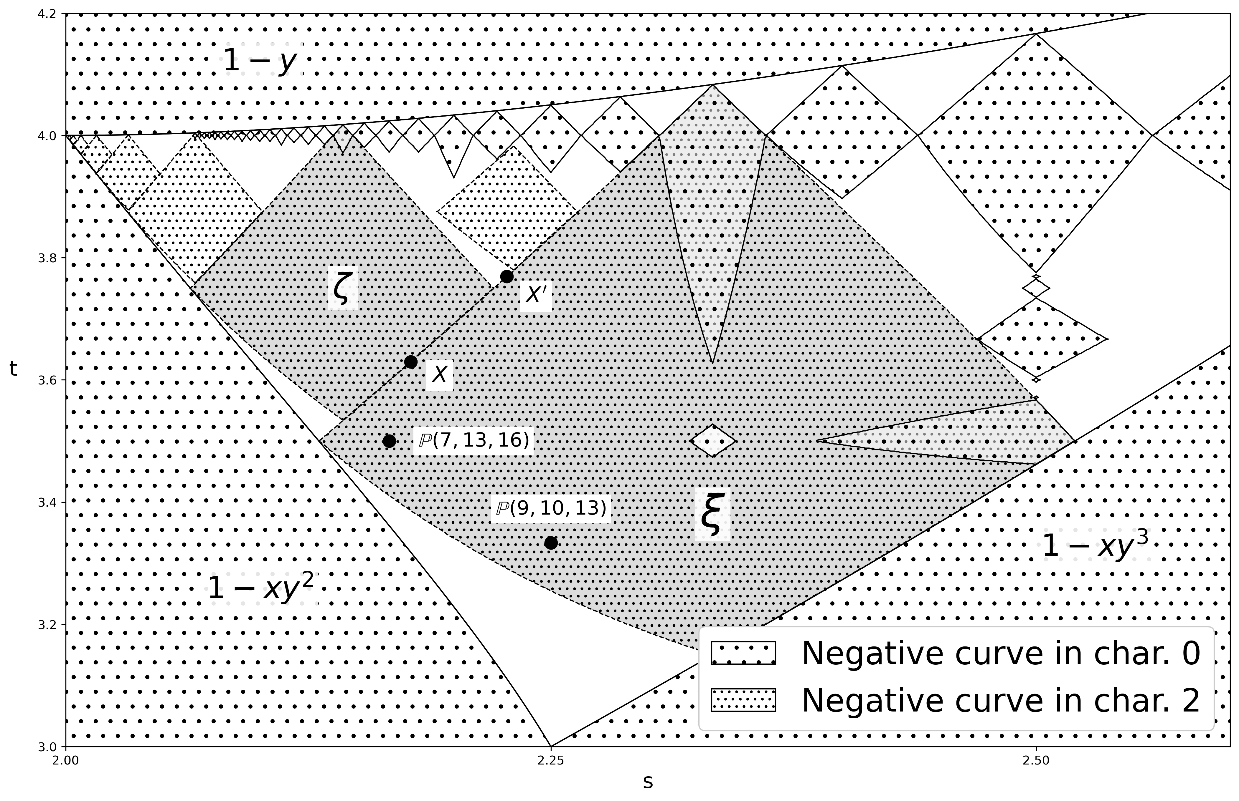
We will use results in characteristic to prove Theorem 1.1. Toric varieties can be defined over a field of any characteristic. The picture of diamonds for each field only depends on the characteristic and not on the field. A polynomial that defines a negative curve in characteristic can be chosen to have integer coefficients. Its reduction mod then defines a (possibly reducible) negative curve in characteristic . Going from characteristic to characteristic , the diamonds may get larger, and there will be new diamonds. Figure 1 shows examples of diamonds of negative curves in characteristic and a few additional diamonds of negative curves in characteristic . The points corresponding to in Theorem 1.1 lie in the intersection of two such diamonds that only exist in characteristic . This means that in characteristic contains two disjoint irreducible curves and , both with self-intersection zero. These curves span an extremal ray of the cone of curves of . In fact, if and are the defining equations of the two curves, then polynomials in give us all curves on this ray. A negative curve for in characteristic must also have self-intersection and hence lie on the same extremal ray (otherwise its reduction mod would give a strictly negative curve in characteristic ). We prove that no polynomial in (except the monomials ) can be lifted to characteristic while preserving the condition of vanishing at to order .
Let us mention three open problems that are related to the existence of negative curves: the Mori Dream Space property in positive characteristic, irrationality of Seshadri constants, and Nagata’s conjecture. The triangles in Theorem 1.1 do not give us new information about these problems. However, a similar study of more general triangles would solve the open problems.
It is known by a result of Cutkosky [4] (see also the algebraic version by Huneke [13]) that is a Mori Dream Space (MDS) if and only if it contains a negative curve and a curve disjoint from it. This result holds even when and have self-intersection zero, see [9, Lemma 2.1]. Thus, the varieties in Theorem 1.1 are MDS in characteristic . In positive characteristic, it is also known [4] that if contains a negative curve with strictly negative self-intersection, then is a MDS. This fact uses the result of Artin that such negative curves are contractible [1]. However, if has self-intersection zero, then it is not known if in positive characteristic is a MDS or not. In fact, we do not know any blowup as above that is not a MDS in positive characteristic. Let be the triangle as in Theorem 1.1 but with . Then in characteristic contains a negative curve of self-intersection zero, defined by the same polynomial as above. We conjecture that contains no curve disjoint from and hence is not a MDS. In Figure 1, the variety lies on the boundary of only one diamond.
Negative curves in are related to Seshadri constants (see the discussion in [3, 5]). Recall that if is an ample divisor on a variety and is a point, then the single point Seshadri constant of is
Here the infimum is over all curves in passing through . It is an open problem to find examples of surfaces where the single point Seshadri constant is irrational (see for example [2, 6, 11] for a survey and more recent work). In our case, , any ample divisor on , the single point Seshadri constant at is the slope (with respect to and ) of the extremal ray in the cone of curves of . If contains a negative curve then the slope is clearly rational. The examples in Theorem 1.1 also have rational slopes because such an contains a negative curve in characteristic and the cones in characteristic and are equal. In general, if does not contain a negative curve, then the extremal ray is generated by a class of self-intersection zero. The slope of this ray can be computed from the triangle, and it is typically irrational. When , then the slope is rational if and only if is a square in . Examples such as the blowups of , are conjectured to contain no negative curve [14]. Such weighted projective planes would then provide examples with irrational Seshadri constants.
Nagata’s conjecture [15] states that if are very general points in and is a curve that has multiplicity at the point , then for ,
| (1.1) |
Nagata [15] proved the conjecture in the case where is a square. A slightly weaker inequality was proved by Xu [17]. A toric variety given by a triangle can always be presented as a quotient of by a finite abelian group. The examples in Theorem 1.1 are quotients by an abelian group of order that is a square. Then a curve in that has multiplicity at can be pulled back to so that it passes through the preimages of with multiplicity . Equation 1.1 applied in this situation says that the strict transform of in has positive self-intersection. In other words, if the inequality holds then has no negative curve. Of course, the points in this case are not very general in the sense of Nagata, so Nagata’s conjecture, which is known in the case where is a square, does not imply Theorem 1.1. However, it is true that Theorem 1.1 is equivalent to Nagata’s inequality for the special set of points in the preimage of . For the converse direction, assume that a curve fails the inequality in (1.1). Then the union of the translates of by the group action is the inverse image of a curve in whose strict transform in has nonpositive self-intersection.
The proof of Theorem 1.1 is organized as follows. We fix one triangle and variety as in the statement of Theorem 1.1. In Section 2 we prove the claim that polynomials in the ring give us all curves of self-intersection zero in the variety in characteristic . In Section 4 we show that none of the curves in characteristic can be lifted to characteristic . We show that the obstruction to this lifting lies in a space of first cohomologies. Section 3 defines , gives it the structure of an -module, and proves that it is a free module. The freeness is then used in Section 4 to show that the relevant obstruction to lifting does not vanish. In Section 5 we present some linear algebra computations. This is the only section where the proofs depend on the specific triangle ; all other proofs work for any triangle in the intersection of the diamonds of and .
We work over the field throughout the paper. The main result, Theorem 1.1, holds over a field of characteristic zero. The background material about toric varieties such as their Weil divisors, class group, vanishing theorems, applies over any ground field.
2. The section ring
Let be a normal variety and Weil divisors on . Define the section ring
If the classes of span the class group , then is called a Cox ring of [12]. In this section we consider a particular section ring of and compute this ring explicitly.
2.1. Weil divisors on .
Toric varieties and their -invariant divisors can be defined over any field (and even over any ring). We start with an arbitrary field, but then specialize to the case of . Let us first recall how to find the class group of a toric variety using its -invariant Weil divisors [7].
Let be a rational triangle in , for example a triangle as in Theorem 1.1. The toric variety is -factorial, meaning that every Weil divisor has a nonzero integer multiple that is Cartier. We can compute the intersection number of two curves by reducing it to the intersection number of a curve and a Cartier divisor.
The class group of is a direct sum of a free group of rank and a finite group. To construct it, one starts with -invariant Weil divisors (-Weil divisors for short), that means, integral linear combinations of the three boundary divisors. The group of -Weil divisors is generated by nef divisors which have a geometric description. A nef -Weil divisor corresponds to a triangle with sides parallel to the sides of and all sides integral in the sense that the affine line spanned by each side contains a lattice point. Addition is defined as the Minkowski sum of triangles.
Two triangles correspond to linearly equivalent divisors if they differ by an integral translation. The class group of is the quotient of the group of -Weil divisors by the linear equivalence relation.
A -Weil divisor defines the sheaf on . This sheaf is locally free if and only if is Cartier, that means, if the corresponding triangle is integral. More precisely, the sheaf is locally free everywhere except at the -fixed points corresponding to non-integral vertices of the triangle. Below we will see several cases where a morphism is an isomorphism or a sequence is exact if the divisors involved are Cartier. In the Weil case this may fail because of a torsion sheaf supported at the -fixed points. (By a torsion sheaf we always mean a coherent torsion sheaf.)
Because a -Weil divisor is supported in the complement of the torus , we have a canonical trivialization of the sheaf on the torus. We can therefore view sections of the sheaf over an open -invariant subset as consisting of Laurent polynomials in with certain vanishing orders along the three boundary divisors.
Given -Weil divisors and in , there is an inclusion of sheaves
The inclusion may not be an equality, but the cokernel is a torsion sheaf supported at the -fixed points. The combinatorial reason why the inclusion may not be an equality is that lattice points in the Minkowski sum of two polyhedra may not be sums of lattice points from the two polyhedra. In the case above, working locally in a -invariant open subset, the polyhedra are rational translates of a cone in .
Given a global section
we let be the closure of the curve that defines away from the three -fixed points. For any -Weil divisor , multiplication with defines a morphism
Lemma 2.1.
Assume that is irreducible and intersects the torus . Then for any the morphism is injective with cokernel
Proof.
The ideal sheaf of is
Tensoring this with gives
The quotients of by these subsheaves now give a surjective morphism
This map is an isomorphism away from the -fixed points, so its kernel is a torsion sheaf. Let us check that has no torsion; hence the kernel consists of all the torsion.
We consider a -invariant open affine . Let be a section of on such that for some section of that does not vanish on , lies in the subsheaf . Recall that we have trivialized all sheaves over the torus, hence we may view all sections as Laurent polynomials. Now, the polynomial divides . Since is irreducible and not a unit, it divides or . In the first case vanishes on , which is not allowed. It follows that must divide . The quotient polynomial is a section of . This last claim follows because sections of are Laurent polynomials with certain vanishing orders at the three boundary divisors. One checks that the quotient has the required orders of vanishing. ∎
2.2. Weil divisors on .
We now fix one triangle as in Theorem 1.1 and compute the class groups of and explicitly. These class groups do not depend on the field over which the varieties are defined.
The triangles defining nef -Weil divisors on are determined by their lower left and right vertices , . The integrality condition of the Weil divisors implies that , and for some nonzero integers . The numbers are the numerators of the slopes , written in lowest terms. The set of triples
is the group of -Weil divisors of .
Lemma 2.2.
For any triangle in Theorem 1.1, either or .
Proof.
Let in lowest terms. Then the slopes and are
not necessarily in lowest terms.
If then , hence . If then and hence . We can divide the numerator and denominator of by . Then . ∎
We will assume below that . If , we can change the roles of the lower left and right vertices. With this assumption, the group of -Weil divisors of can be expressed as the set of triples
where is the length of the base. The class group of is the quotient by the group acting on by integral translation. Thus
The numerical equivalence class of a nef divisor is given by the size of the triangle, that means by .
Let . Then its class group is
where is the class of the exceptional divisor. We write a class as a triple .
For the rest of this section we work over the field . We start by constructing two irreducible disjoint curves and in with zero self-intersection. Recall that we have fixed a variety as in Theorem 1.1, where the triangle is determined by its left vertex . Let be the blowup morphism.
Lemma 2.3.
Let be the -Weil divisor on corresponding to the triangle . Then there exists a nonzero section
that defines an irreducible curve with zero self-intersection. The curve passes through the -fixed points corresponding to the lower left and right vertices of .
Proof.
Let be the reduction mod of the polynomial
The Newton polygon of is the triangle with vertices . This triangle lies in as required. It also follows that is irreducible because its Newton polygon has sides of lattice length , and hence is not the Minkowski sum of smaller integral polygons [8, Lemma 2.1]. When changing coordinates, we get
Clearly all terms of degree less than vanish mod , hence defines a global section of . Since has multiplicity exactly at , the curve that it defines does not have as a component and hence is irreducible. The self-intersection number of is zero:
Because the triangle is not integral at the lower two vertices, the curve passes through the corresponding -fixed points. ∎
Lemma 2.4.
Let be the -Weil divisor on corresponding to the triangle with lower vertices . Then there exists a nonzero section
that defines an irreducible curve with zero self-intersection. The curve passes through the -fixed point corresponding to the top vertex of .
Proof.
We will construct the polynomial with Newton polygon equal to the triangle with vertices . This triangle lies in the triangle with the same base and sides parallel to . Since the left and right sides of the Newton polygon have lattice length , it follows that such is irreducible, and since the top vertex of the triangle with sides parallel to is not integral (it has -coordinate ), the curve defined by passes through the corresponding -fixed point. The self-intersection number of is zero as before.
Let be as in the previous lemma and define to be
Both terms in the sum have all nonzero monomials supported in the triangle defined above, except the monomial . However, these terms cancel in the sum. This shows that is supported in the correct triangle. Clearly both terms of the sum vanish to order at , hence defines a global section of . One checks that the coefficients of the monomials corresponding to the vertices are nonzero, which implies that is nonzero and has the stated Newton polygon.
We also need to check that the curve in does not contain as a component. In other words, that vanishes to order exactly at . If the vanishing order were greater, then would define a negative curve in with strictly negative self-intersection, and that would contradict the existence of the irreducible curve of zero self-intersection defined by . ∎
Figure 1 shows the diamonds of the polynomials and . The point corresponding to any as in Theorem 1.1 lies in the intersection of these two diamonds. It follows from Theorem 2.6 below that and are the only nonzero global sections of their respective sheaves. This gives the uniqueness of the curves and in their linear equivalence classes.
For later use, let us consider , the lifting of , and write
where consists of terms of degree less than and of degree or greater. The proof of Lemma 2.3 shows that
Similarly, we lift to a polynomial and write
where has terms of degree less than and of degree at least . The lowest degree terms of mod lie in degree .
Let us study the curve further. Its intersection number with the exceptional divisor is . This intersection is defined by the vanishing of the lowest degree terms in , namely the homogeneous polynomial . If we dehomogenize it, we get a single variable irreducible polynomial . Thus, if we consider as a scheme over , its intersection with is a single point with residue field . On the other hand, if we consider as a variety over , then this point splits into three distinct points. Since these are simple points on , it follows that is smooth at these points and intersects transversely.
2.3. A section ring of .
We continue working over . Consider the extremal ray of the cone of curves of that contains and . The elements of that have their numerical equivalence classes on this ray satisfy
The equality here is the condition that equals twice the area of the triangle, hence the class has self-intersection zero. The inequality restricts this line to the ray of nef divisors. We may write this subset of as
Let us choose Weil divisors such that the classes of and generate this semigroup:
The triangle of the divisor is the point . The triangle of has lower vertices .
Definition 2.5.
Define the section ring
More concretely, is a graded ring. To find its elements of degree , we consider the triangle with left vertex and base of length . Then the homogeneous part of degree in consists of all Laurent polynomials in that are supported in the triangle and vanish to order at least at .
Note that and are homogeneous elements of . The element lies in degree , and lies in degree . The polynomial lies in degree .
Theorem 2.6.
The elements , and of are algebraically independent over and
Proof.
Let be a homogeneous element of in degree . If the top vertex of the triangle corresponding to this degree does not lie in the Newton polygon of , then the curve passes through the corresponding -fixed point. We know that also passes through this point. Since and is irreducible, it follows that divides as a Laurent polynomial, and hence it divides in the ring .
Similarly, if the Newton polygon of does not contain the left or the right vertex of the triangle, then divides in .
If all three vertices lie in the Newton polygon of , then the triangle must be integral. This implies that and for some . Now, is supported in the same triangle and the difference has Newton polygon that does not contain the left and right vertices; hence we can continue dividing by .
By induction, this process stops when . In this case the triangle is reduced to a point with coordinates . In this degree there is a nonzero global section if and only if the point is integral, . Then is the unique nonzero global section.
The previous argument shows that every element can be written as a polynomial in . Hence the graded morphism
is surjective. We will show that it is also injective. Since the morphism is graded, its kernel must be homogeneous. Suppose the map in degree is not injective. The degree part of the left hand side has a basis consisting of all monomials
such that and . We will consider the Newton polygons of these monomials restricted to the -axis, . The Newton polygons of and restrict to intervals and , respectively. The Newton polygon of is simply the point . From this we can compute the Newton polygon of the monomial to be
Notice that the left endpoints of these intervals increase with since . Hence if there is a relation among the monomials, then one proves by induction on that the coefficients in front of the monomials must all be zero. ∎
3. The module of first cohomologies.
We fix a variety as in Theorem 1.1. In the previous section, we defined the ring of zeroth cohomologies of certain sheaves. In this section we define similarly the space of first cohomologies of the same sheaves. This has the structure of an -module. In the next section we prove that no element of can be lifted to characteristic zero. The obstruction to lifting lies in the module .
We work over the field throughout this section. The computation of cohomology in the next subsection works over any field.
3.1. The first cohomology
Let be a -Weil divisor on , , and the blowup morphism. We consider the divisor
on . Global sections of can be identified with global sections of that vanish to order at least at . Let us write this more formally.
Let be the closed subscheme of the torus defined by the ideal . Consider the restriction of the sheaf to the subscheme :
where the last equality follows from the trivialization of the sheaf on the torus. This morphism induces a morphism of global sections
which can be described more concretely as follows. A global section on the left hand side is a Laurent polynomial in and . The map takes it to
Lemma 3.1.
The kernel and cokernel of are and , respectively.
Proof.
There is an exact sequence of sheaves on
where is the -fold thickening of . This gives an exact sequence of cohomology
The sequence ends on the right because is a nef -Cartier divisor on a toric variety, hence its higher cohomology vanishes [7]:
In the exact sequence of global sections, the middle map can be identified with . ∎
Remark 3.2.
Lemma 3.1 was stated for the variety over the field , but clearly it holds for over any field. Note also that we can represent the map by an integer matrix that does not depend on the field. This is done by choosing the basis of monomials in both source and target. In Section 4 below, we will in fact define over any base ring . Working over an arbitrary field, the kernel and cokernel of are defined over the prime field, in characteristic and in characteristic . Consider the case where is nonzero over a field of characteristic . Then we may choose a nonzero element in the kernel as a polynomial with rational coefficients, and after clearing denominators, we may assume further that the coefficients are integers with of all coefficients equal to . Such a polynomial defines a nonzero element in in characteristic that reduces to a nonzero element in characteristic .
3.2. The module .
Recall that we defined the section ring graded by :
We define similarly the space of first cohomologies:
The graded vector spaces and can be put into an exact sequence
where is a -Weil divisor on such that
Let now be a homogeneous element of in degree . Then multiplication with defines a graded morphism of degree of the exact sequence above:
| (3.1) |
These multiplication maps give the structure of a graded -module. Recall that , where and are defined in Lemma 2.3 and Lemma 2.4,
The action of and on is by multiplication with and , respectively. The variable acts by multiplication with . The inverse acts by multiplication with . This is well defined because on each graded piece of multiplication with is zero for large enough.
Theorem 3.3.
The module is a graded free -module.
3.3. Proof of Theorem 3.3.
We show that form an -regular sequence. This implies that is a graded free -module. The element acts on by a graded isomorphism. This action turns into a free -module, which implies that is a free -module.
Lemma 3.4.
The element is not a zero-divisor on .
Proof.
Consider the map of exact sequences (3.1) defined by . We restrict this map to one degree so that it goes from degree to degree , . Write the divisors in these degrees as
We add the kernels and cokernels of the vertical maps to the diagram. Then, with some abuse of notation, we have
It is easy to see that the kernels in the left three columns are all zero. In the second column, the map is multiplication in the Laurent polynomial ring. Since this ring is a domain, the kernel of this map, as well as the kernel in the first column, is zero. In the third column, if , then using the fact that lies in , we get that .
The diagram gives us a sequence of maps of the cokernels
This sequence is exact except possibly at ,
(This can be seen by cutting the two rows into two short exact sequences and then considering the two long exact sequences of kernels and cokernels.) Thus, to show that , we need to prove that the sequence is also exact at . We will describe the three spaces .
The space is the quotient in degree . This is either zero or -dimensional with basis when and .
To find , by Lemma 2.1 we have an exact sequence of sheaves
Here , and is its strict transform in . We assume that , hence is a nef divisor on and the higher cohomology of vanishes. Then the cohomology sequence of the short exact sequence gives us
The sheaf is locally free in a neighborhood of if and only if the left and right vertices of the triangle corresponding to are integral. This is equivalent to and . (Notice that this is the same condition as the one for to be nonzero.) In this case restricts to a degree line bundle on .
In general, is a Cartier divisor in a neighborhood of for some integer . The sheaf restricts to a degree line bundle on . We will use the inclusion
as follows. Given an element , gives a global section of the line bundle . If is not Cartier at a -fixed point on , then the section vanishes at that point.
The space is the coordinate ring of the affine scheme .
Now consider . This is a global section of that vanishes on . We claim that the vanishing imposes conditions on the sections . Since we have trivialized on the torus, this does not depend on the divisor . We may assume that and work with functions in . Functions on can be pulled back to functions on . If a function on vanishes on , then its pullback vanishes on . When working over , the curve intersects transversely at points. Hence the pullback of must vanish at points on when counted with multiplicities. This imposes linear conditions on sections . Note also that the map is a linear map defined over the field . Its rank does not change if we extend the field to .
First consider the case where is Cartier in a neighborhood of . Then the pullback of to is a line bundle of degree . The pullback of gives a section of this bundle that vanishes at points. There can be at most one such nonzero section, so that has dimension at most . In this case we know that has dimension . It follows that .
If is not Cartier in a neighborhood of , consider the section pulled back to for some such that is Cartier. This pullback is a global section of a degree line bundle that vanishes at points in . Since is not Cartier, also vanishes at a -fixed point on . This implies that . In this case also , hence . ∎
Lemma 3.5.
The element is not a zero-divisor on .
Proof.
The degree part of the quotient module was called in the proof of the previous lemma. In the same lemma we constructed an exact sequence
and described the other terms for explicitly. We will now consider two such exact sequences of in degrees and . Multiplication with takes one sequence to the other. On the terms this gives the action of on . Let us denote the divisors in degrees and
We will assume that , otherwise the source is zero. The morphism of the two exact sequences with kernels and cokernels added is:
Here we have used subscripts to denote the degree. Again, it is not hard to check that the kernels of the left three vertical maps are zero. In the second column this follows because we are multiplying sections of torsion-free sheaves on an irreducible curve.
To prove that the third vertical map is injective, we will change the ground field from to , which allows a more geometric argument. Since is a linear map between -vector spaces, its injectivity does not change if we extend the field. We work over and consider regular functions on pulled back to regular functions on . This defines an inclusion
The pullback of to the blowup defines the divisor , and since does not intersect , multiplication by the pullback of is the multiplication by a local equation of . This multiplication is injective. Locally at each of the points in , the map is isomorphic to
where is the local equation of , defining a local parameter for .
We also note that the cokernel is zero in degree because . This gives us an exact sequence
and we need to prove that is injective. We do this by describing and geometrically.
Let be the curve defined by , so that is its strict transform in . The space is the coordinate ring of the affine scheme . This scheme is equal to . Indeed, in the blowup , the scheme defined by the vanishing of and is
To find the space , we start with the exact sequence
Restriction of these sheaves to gives an exact sequence
There is no term on the left because is a complete intersection in . There is also no need to mention the torsion on the right because is supported at the point while the torsion was supported at a -fixed point. The left two sheaves may have torsion at the two -fixed points that lie on . We can mod out by this torsion and consider the long exact sequence in cohomology:
The cokernel of in this sequence gives the space . Note that
This inclusion is the map in the sequence above. ∎
4. Proof of Theorem 1.1.
We fix one variety . Suppose by contradiction that over a field of characteristic contains a negative curve. As explained in Remark 3.2, we may assume that this curve is defined by a polynomial with integer coefficients such that the reduction of mod gives a possibly reducible negative curve in characteristic . We know that all such must lie in the ring , hence is a lift of the element to characteristic . To prove Theorem 1.1, we show that no element of in degree can be lifted to characteristic zero.
For any ring S, define and by the exact sequence of graded maps of -modules
Here consists of Laurent polynomials with coefficients in and supported in the triangle corresponding to the degree . In the third term,
and is the change of coordinates map
We are interested in the cases where or . The case gives the previously defined and .
The definition of is functorial in . We say that an element lifts to characteristic zero if lies in the image of . More generally, given , we say that lifts mod for if it lies in the image of . Clearly, if an element lifts to characteristic zero then it lifts mod for any .
For an integer , define its -adic order, , as the largest such that divides . The element has order . For a polynomial with integer coefficients, we define similarly its order as the largest such that divides all its coefficients. If the polynomial has order , we call its initial terms the sum of those terms that have coefficients with order exactly . A polynomial has infinite order if and only if it is the zero polynomial. In that case its initial terms are also zero.
Lemma 4.1.
Let be such that lies in the kernel of :
for some , , and hence defines an element . Then can be lifted to mod if and only if maps to zero in .
Proof.
To lift means to find such that
This congruence holds if and only if
which means in . ∎
We start by considering liftings of the generators and of . For the rest of this section let us fix representatives , and write these as
where , , , . Here we view as elements of the same degree as , either in , where , or in the quotient . Multiplication with gives the action of .
From the previous lemma we get that (resp. ) can be lifted mod if and only if the image of (resp. ) is zero in .
Let us also consider liftings of (the case of is similar). We use the same integral representation . Then
Here , hence the first term tells us that automatically lifts mod . The image of in determines if can be lifted mod :
One can ask if, more generally, we can lift mod by adding a multiple of to :
However, notice that , and since is the only nonzero element of in its degree, we must have for some . We saw that , hence . Therefore, adding the term does not change the liftability of mod . In summary, can be lifted mod if and only if in zero in .
Lemma 4.2.
The elements are nonzero in . In other words, can not be lifted mod , and can not be lifted mod .
We will prove Lemma 4.2 in the next section. The proof of this lemma is the only part in the proof of Theorem 1.1 that depends on the triangle . All other proofs work the same way for all triangles.
Theorem 4.3.
Let be a nonzero homogeneous element of degree that lifts to characteristic zero. Then, there is a nontrivial linear relation:
between elements , where
Proof.
Let
and let be a lifting of to characteristic zero; that means, an integral polynomial in that lies in the kernel of and reduces to mod . We lift the coefficients of to and write
The liftings are chosen so that , written as a Laurent polynomial in , is as close to as possible, namely the difference
has maximal order. We first check that such an with maximal order exists: if there is a sequence of with increasing orders then we may also take with infinite order. Let be the free -module generated by the finite set of monomials in degree , and let
be the -linear map that writes a polynomial in as a Laurent polynomial in . Then is injective. We showed this in the proof of Theorem 2.6 over , and this implies it over . Now suppose we have a sequence of such that the sequence approaches in the -adic topology (the differences have orders approaching infinity). Since the subspace is closed in the -adic topology, the sequence also approaches a limit . Now if we take , then and .
The orders satisfy:
- (1)
because .
- (2)
because has infinite order, so the initial terms of and must cancel.
- (3)
. Change of coordinates does not change the order, but when applying we also remove the higher degree terms.
- (4)
. This is clear if . Otherwise, let , for some . If then . Hence is a nonzero element of . Since is a polynomial in , we can move such terms from to and increase the order of .
These conditions imply
We now consider the initial terms in the expression . Since the left hand side is zero, the initial terms of and must sum to zero. We claim that has finite order and
where the linear combination is as in the statement of the theorem. (For simplicity, here and below we are abusing notation slightly. The sum in the parentheses is an element of that mod reduces to the claimed expression.) Assuming this, also has the same finite order , and we can write . The theorem now follows from the congruence
We prove the claim about the initial terms of by the following steps:
- (1)
For every monomial that can appear in , we show that has a finite order that depends on . Moreover,
where the linear combination mod is as in the statement of the theorem.
- (2)
For different monomials , the expression has different but the same . A linear combination of such expressions is then an expression of the same type.
- (3)
The coefficients that appear for different monomials are linearly independent over . This implies that a nontrivial linear combination of the expressions for different monomials is a nontrivial linear combination of and . The initial terms of are then times one such nontrivial linear combination, where is finite.
Consider one monomial . We will find the initial terms of . The order of is . Its initial terms mod are . Next consider :
When is odd, we get
and when is even, we get
There are similarly two cases for depending on whether is odd or even. When computing the initial terms of , we get four cases depending on the parity of and . In the first case, where and are both odd,
Since , we get the initial terms
Here we view as a linear combination of elements and with coefficients and . The polynomials correspond to elements and in .
In the second case, when is even and is odd, then
Here we have a linear combination with only one term , where and . The case odd, even, gives similarly a one term linear combination.
Finally consider the case where both and are even. If the orders of and are not equal, then we get a linear combination with one term. Let us do the more complex case when . Then
Here we have a linear combination of and with coefficients and . (When the orders of and are not equal, we get one half of this linear combination, or .)
Notice that all monomials in the same degree must have the same parity of and the same parity of . This can be seen by finding all Laurent monomials of degree . These monomials are all powers of . The fact that and are even then proves the claim. This implies that the expressions that we get for each monomial involve the same and . Hence a linear combination of these expressions is an expression of the same type.
Finally, let us prove that the coefficients that appear in the expression for different monomials are linearly independent over . This is easy to see from the formulas above. For example, suppose the degree is such that both and are even. Then the coefficients for a monomial are either or or . These three cases correspond to , , and . Since the monomials are linearly independent in , these vectors in as vary are clearly linearly independent. ∎
Recall that and are graded by . In the next theorem we only need the second component of the degree. Let us simply call this the degree.
Theorem 4.4.
Let be nonzero homogeneous elements, in degree or , and in degree or . Then there is no nontrivial relation
in with coefficients .
Proof.
We will use the fact that is a free -module. In particular, it is a flat -module. The flatness criterion applied to the relation above states that there exist elements and such that
Since are homogeneous, we may assume that the relation above is also homogeneous. Then we may choose and homogeneous such that if then .
Consider the degrees of nonzero elements in and . First we claim that is zero in degree . Indeed, is a quotient of , and this space is zero in degree . The ring has nonzero elements in degrees .
For each consider the possible degrees of that are involved in the equality ; that means, such that . Considering the possible degrees of , we get the possible degrees of as:
Since no can appear in both and , it follows that for all . This implies that both and . ∎
The previous two theorems complete the proof of Theorem 1.1.
5. computations
We now prove Lemma 4.2. The proof reduces to linear algebra computations. Since the matrices are large (up to size ), these are best done on a computer. We have used the Sage system [16].
To explain the idea, let us prove the lemma first for a specific defined by . We will then do the same for all .
Let us start by proving that is not zero in . By Lemma 4.1, this is equivalent to not having a lift mod . Since is the only nonzero element in in its degree, it is also equivalent to saying that the only elements of in the same degree as are divisible by .
Let be the integer matrix that represents in the degree of over . We need to show that every integer vector such that is divisible by . Recall that the matrix can be put in the Smith normal form (by viewing as a linear transformation and choosing bases for the source and the target) so that the matrix becomes diagonal. The diagonal entries are the elementary divisors of . These can be computed in Sage with the command L.elementary_divisors(). We know that the matrix has a -dimensional kernel mod , hence there is one elementary divisor divisible by . We need to check that this divisor is not divisible by . This can be verified by computing the elementary divisors:
The matrix is constructed as follows. It has columns indexed by lattice points in the triangle and rows indexed by lattice points in the triangle with vertices . The entry in row and column is
In Sage it is convenient to give a polygon by its vertices and then list all its lattice points with a single command, for example:
| Polyhedron(vertices=[(-3/14,0),(15/14,0),(3,7)]).integral_points() |
Next, is nonzero in if and only if cannot be lifted mod . As in the case of , this is equivalent to saying that all elements of in the same degree as are divisible by . Let be the matrix representing in the degree of . The elementary divisors of computed in Sage are:
The matrix in this case has size . If the matrix has more rows than columns then the list of diagonal entries in its Smith normal form is padded with zeros. These zeros correspond to the free part of . Since we are interested in the kernel of , we may ignore these trailing zeros. There is exactly one (nonzero) elementary divisor divisible by , confirming that . Since this elementary divisor is not divisible by , it follows that every element in the kernel of mod is divisible by , hence cannot be lifted mod .
Similarly, the proof that and in is reduced to computing the elementary divisors. In the case of the matrix is and has elementary divisors:
and in the case of :
In the last case, the matrix has size and just as before we may ignore the trailing zeros. The fact that is not divisible by and is not divisible by proves that and are nonzero in .
5.1. General triangles .
It suffices to prove that and do not lift mod 8 no matter which triangle we consider. The case of and follows from this. For example, if lifts mod then by the same argument as in Section 4, automatically lifts mod .
Let us start with . We need to show that the triangle of does not support an integral polynomial such that and . It suffices to prove this for a larger polygon that contains the triangle of . Indeed, if we can find such supported in the triangle, then the same is also supported in the larger polygon. We can thus choose a polygon that contains some (or even all) of the triangles that we are considering. Then proving that the polygon does not support such proves it for all these triangles.
We are interested in triangles with . We divide this set of into two subintervals:
The triangles of for the first set of all lie in a larger triangle with vertices
and for the second set of they lie in a larger triangle with vertices
We will now consider the map from polynomials supported in twice these two larger triangles to , and compute its elementary divisors. In both cases the matrix has size and the elementary divisors are the same:
| [1, ...,1,4] |
Since does not divide any elementary divisor, this shows that can not be lifted mod for any triangle .
Next we do the same computation for . The triangles of have vertices
where ranges in the interval . We divide this interval into subintervals with vertices at
Then the triangles corresponding to the -th subinterval, , lie in a trapezoid with vertices
We consider the map from polynomials supported in twice the trapezoid to . We list the size of the matrix and the elementary divisors in each of the four cases:
The size of the matrices tells us that we may ignore the trailing zeros. Since the nonzero elementary divisors are not divisible by , this shows that cannot be lifted mod for any triangle . ∎
References
- [1] Michael Artin. Some numerical criteria for contractability of curves on algebraic surfaces. American Journal of Mathematics, 84(3):485–496, 1962.
- [2] Thomas Bauer, Sandra Di Rocco, Brian Harbourne, Michał Kapustka, Andreas Knutsen, Wioletta Syzdek, and Tomasz Szemberg. A primer on Seshadri constants. Contemporary Mathematics, 496:33, 2009.
- [3] Ana-Maria Castravet. Mori dream spaces and blow-ups. In Tommaso de Fernex, Brendan Hassett, Mircea Mustaţă, Martin Olsson, Mihnea Popa, and Richard Thomas, editors, Algebraic Geometry: Salt Lake City 2015, volume 97.1 of Proceedings of Symposia in Pure Mathematics, pages 143–168. American Mathematical Society, 2018.
- [4] Steven Dale Cutkosky. Symbolic algebras of monomial primes. J. Reine Angew. Math., 416:71–89, 1991.
- [5] Steven Dale Cutkosky and Kazuhiko Kurano. Asymptotic regularity of powers of ideals of points in a weighted projective plane. Kyoto Journal of Mathematics, 51(1):25–45, 2011.
- [6] Marcin Dumnicki, Alex Küronya, Catriona Maclean, and Tomasz Szemberg. Rationality of Seshadri constants and the Segre–Harbourne–Gimigliano–Hirschowitz conjecture. Advances in Mathematics, 303:1162–1170, 2016.
- [7] William Fulton. Introduction to toric varieties, volume 131 of Annals of Mathematics Studies. Princeton University Press, Princeton, NJ, 1993. The William H. Roever Lectures in Geometry.
- [8] Javier González Anaya, José Luis González, and Kalle Karu. Constructing non-Mori Dream Spaces from negative curves. J. Algebra, 539:118–137, 2019.
- [9] Javier González Anaya, José Luis González, and Kalle Karu. On a family of negative curves. J. Pure Appl. Algebra, 223(11):4871–4887, 2019.
- [10] Javier González-Anaya, José Luis González, and Kalle Karu. The geography of negative curves. arXiv preprint arXiv:2104.03950, 2021.
- [11] Krishna Hanumanthu and Brian Harbourne. Single point Seshadri constants on rational surfaces. Journal of Algebra, 499:37–42, 2018.
- [12] Yi Hu and Sean Keel. Mori dream spaces and GIT. Michigan Math. J., 48:331–348, 2000. Dedicated to William Fulton on the occasion of his 60th birthday.
- [13] Craig Huneke. Hilbert functions and symbolic powers. Michigan Math. J., 34(2):293–318, 1987.
- [14] Kazuhiko Kurano and Naoyuki Matsuoka. On finite generation of symbolic Rees rings of space monomial curves and existence of negative curves. J. Algebra, 322(9):3268–3290, 2009.
- [15] Masayoshi Nagata. On the 14-th problem of Hilbert. American Journal of Mathematics, 81(3):766–772, 1959.
- [16] The Sage Developers. SageMath, the Sage Mathematics Software System (Version 9.3), 2021. https://www.sagemath.org.
- [17] Geng Xu. Curves in P2 and symplectic packings. Mathematische Annalen, 299(1):609–613, 1994.