Quantum fluctuations and correlations in open quantum Dicke models

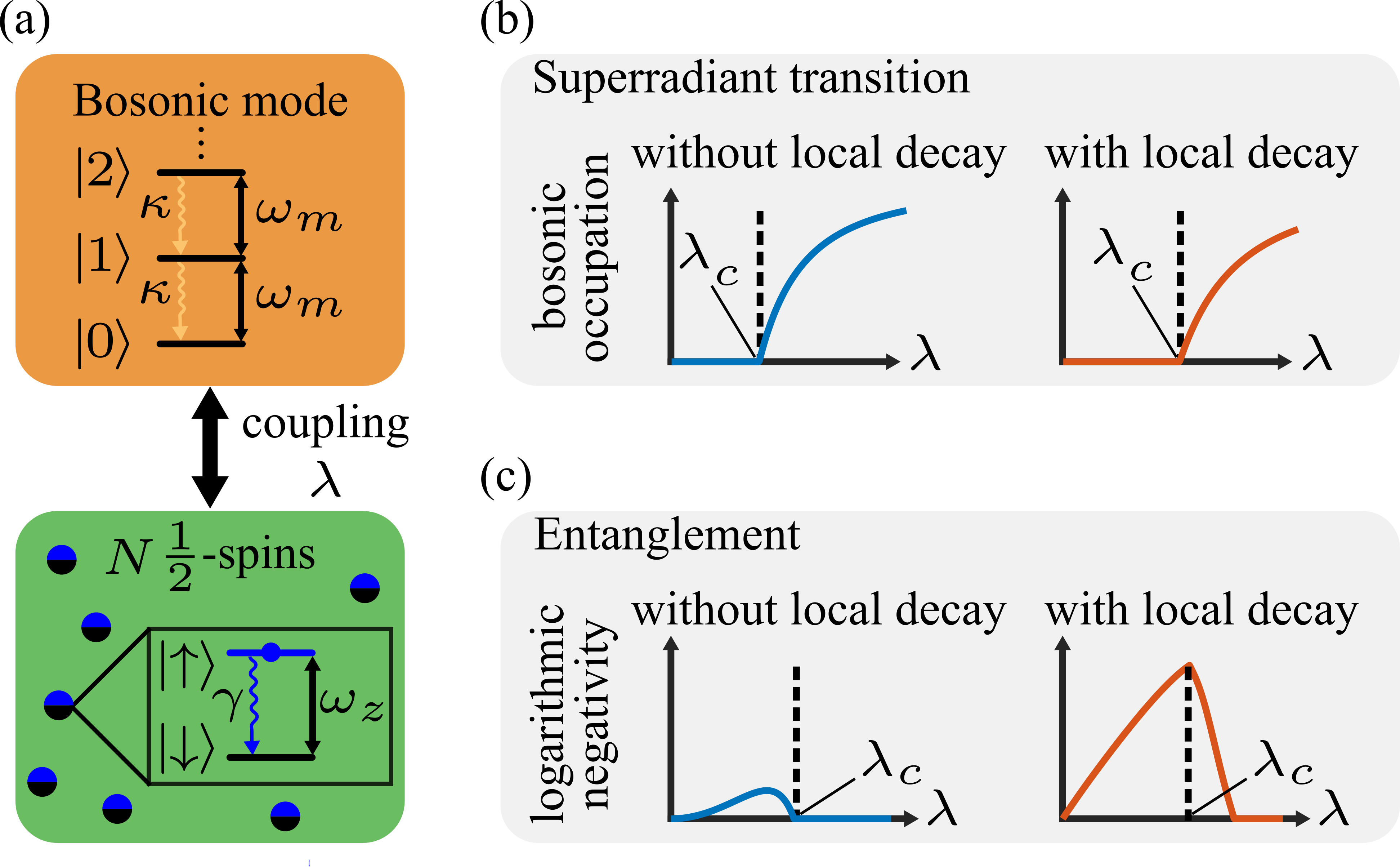
Spin-boson models are paradigmatic theoretical models describing, for instance, the coupling of matter with electromagnetic fields or vibrational modes. A prominent example is the so-called Dicke model Dicke 1954, which provides a simple framework for the study of the interaction between a large ensemble of atoms, described by $N$ spin-1/2 (two-level) particles, and an electromagnetic cavity field, described by a bosonic mode [cf. Fig. 1(a)]. This model has been thoroughly investigated in equilibrium Hepp and Lieb 1973a; Hepp and Lieb 1973b; Wang and Hioe 1973; Hioe 1973; Carmichael et al. 1973; Duncan 1974, where it displays a second-order ground-state transition from a normal to a superradiant phase. While the order-parameter behavior is captured by a mean-field treatment Kirton et al. 2019, studying quantum correlations requires the analysis of quantum fluctuations Emary and Brandes 2003a; Emary and Brandes 2003b; Lambert et al. 2004; Lambert et al. 2005; Soldati et al. 2021. In equilibrium, this is typically done within the so-called Holstein-Primakoff approximation Holstein and Primakoff 1940. This exploits that the system Hamiltonian can be written in terms of collective (macroscopic) spin operators, which approximately behave as bosons when the system is close to its ground-state.

Nowadays, also due to a debate concerning a no-go theorem on the experimental realization of the equilibrium Dicke model Rzażewski et al. 1975; Bialynicki-Birula and Rzażewski 1979; Keeling 2007, the focus is on the investigation of Dicke physics in an open quantum system setting [cf. Fig. 1(a)]. Open Dicke models feature a nonequilibrium superradiant phase transition, see Fig. 1(b), which is exactly captured by a mean-field approach Kirton and Keeling 2017; Carollo and Lesanovsky 2021. However, in these settings, analyzing quantum fluctuations is challenging Kirton et al. 2019; Sieberer et al. 2016; Dalla Torre et al. 2013; Buča and Jaksch 2019. As a consequence, very little is known about correlations in the nonequilibrium Dicke model phase transition, and even less in the presence of local dissipative processes, such as local spin-decay [cf. Fig. 1(a)].

In this paper, we provide a complete characterization of quantum and classical correlations in open quantum Dicke models. We achieve this by developing an approach for treating quantum correlations, which is based on the theory of quantum fluctuation operators Goderis et al. 1989; Goderis and Vets 1989; Goderis et al. 1990; Verbeure 2010; Benatti et al. 2017; Benatti et al. 2018, that can be applied also in cases where the Holstein-Primakoff approximation cannot be exploited, e. g. in the presence of local dissipative terms which prevent a representation of the dynamics through collective spin operators. We focus on various correlation measures, such as quantum discord and classical correlation, and show that they display non-analytic behavior at the critical coupling strength [see e. g. Fig. 1(c)]. Furthermore, we analyze bipartite entanglement between the spins and the bosonic mode. We find that the presence of local spin-decay — an unavoidable process in experiments which is usually considered detrimental for quantum effects — is unexpectedly beneficial for the build-up of quantum correlations. Our results indicate that this process leads to increased entanglement in the normal phase, and to the emergence of a nonequilibrium superradiant phase [cf. Fig. 1(c)] where entanglement is nonvanishing.

The system is governed by a Markovian open quantum dynamics, under which the time-evolution of an operator $O$ follows the Lindblad equation $\dot{O}(t)=\mathcal{L}_{N}[O(t)]$ Breuer and Petruccione 2002; Lindblad 1976; Gorini et al. 1976 with generator

The first term on the right-hand side of Eq. (Quantum fluctuations and correlations in open quantum Dicke models) gives the coherent contribution to the dynamics implemented by the Dicke Hamiltonian (setting $\hbar=1$)

Here, $\omega_{m}>0$ is the bosonic mode frequency, $\omega_{z}>0$ the energy splitting between spin states and $\lambda>0$ the coupling parameter [cf. Fig. 1(a)]. The Dicke Hamiltonian (2) is written in terms of the collective operators $S^{\alpha}=\sum^{N}_{k=1}\sigma^{\alpha}_{k}$, obeying $[S^{\alpha},S^{\beta}]=i\sum_{\gamma}\epsilon^{\alpha\beta\gamma}S^{\gamma}$, where $\epsilon^{\alpha\beta\gamma}$ is the Levi-Civita symbol. The factor $1/\sqrt{N}$, which rescales the collective spin-boson coupling in $H_{N}^{D}$, is necessary for a well-defined thermodynamic limit Kirton et al. 2019. The last two terms in Eq. (Quantum fluctuations and correlations in open quantum Dicke models) account for irreversible dynamical effects. These are decay of bosonic excitations at rate $\kappa$ as well as local (individual) spin-decay, $\ket{\uparrow}\to\ket{\downarrow}$, at rate $\gamma$. As becomes clear from Eq. (Quantum fluctuations and correlations in open quantum Dicke models), the latter process is not described through collective, but rather local, spin (jump) operators $\sigma^{-}_{k}$.

The form of the order parameter suggests the definition of the so-called mean-field operators

where the last term must be considered for $\alpha=x,y,z$. The first two operators are relevant as they provide the order parameter through $(m_{N}^{q})^{2}+(m_{N}^{p})^{2}-1/N=2a^{\dagger}a/N$. The mean-field operators of the spin ensemble [last terms in Eqs. (3)] are also important for studying the model. Indeed, by computing the action of the generator $\mathcal{L}_{N}$ in Eq. (Quantum fluctuations and correlations in open quantum Dicke models) on the mean-field operators in Eqs. (3), one finds that these operators are all dynamically coupled Carollo and Lesanovsky 2021. In the thermodynamic limit, the time-evolved operators $m_{N}^{\alpha}(t)$ (with $\alpha=x,y,z,q,p$) behave as multiples of the identity proportional to their expectation, i. e. $m^{\alpha}_{N}(t)\to m^{\alpha}(t)=\lim_{N\to\infty}\langle m_{N}^{\alpha}(t)\rangle$ Kirton and Keeling 2017; Carollo and Lesanovsky 2021. Furthermore, they obey the differential equations (we drop the explicit time-dependence)

These equations feature two different stationary regimes, separated by a critical value of the coupling strength

For $\lambda<\lambda_{c}$, there exists a unique stable stationary solution to the system in Eqs. (4), with the only nonzero value given by $m^{z}=-1/2$. This is the normal phase. For $\lambda>\lambda_{c}$, this becomes unstable but two other stable solutions emerge which spontaneously break the symmetry $a\to-a$, $\sigma^{-}\to-\sigma^{-}$ of the generator $\mathcal{L}_{N}$ Kirton et al. 2019; Roses and Dalla Torre 2020; SM.Hurwitz 1895; Khalil 2002; Gantmacher 1959; Horn and Johnson 1991; Behr et al. 2019; Simon et al. 1994; Simon et al. 1987 These feature finite stationary values of $m^{x/p}$, which imply a macroscopic occupation of the bosonic mode in this superradiant phase. (Details are provided in the Supplemental Material SM.)

The fluctuation operators read

For $\alpha=x,y,z$, these are the usual spin fluctuation operators Benatti et al. 2017; Benatti et al. 2018, and we have defined the bosonic ones ($\alpha=q,p$) in full analogy. Roughly speaking, the operators in Eqs. (6) account for deviations of the operators $m_{N}^{\alpha}$ from the mean-field behavior. Remarkably, despite being collective, these retain a quantum character in the thermodynamic limit, in which the limiting operators $F^{\alpha}=\lim_{N\to\infty}F^{\alpha}_{N}$ behave as bosons (for a rigorous discussion see e. g. Ref. Verbeure 2010). This is straightforward to check for $F^{q/p}$, since $F_{N}^{q}=q-\langle q\rangle$ and $F_{N}^{p}=p-\langle p\rangle$. However, also collective spin fluctuations give rise to an emergent bosonic mode. This can be seen as follows. Looking at the commutator of fluctuation operators, one finds that $[F^{\alpha},F^{\beta}]=i\sum_{\gamma}\epsilon^{\alpha\beta\gamma}m^{\gamma}$ ($\alpha,\beta=x,y,z$), which is a multiple of the identity. Now, we rotate the reference frame for the spin ensemble aligning the $z$-direction with the direction identified by mean-field variables, which is $\hat{n}=\vec{m}^{s}/|\vec{m}^{s}|$ with $\vec{m}^{s}=(m^{x},m^{y},m^{z})^{T}$. In this rotated frame we have $\tilde{m}^{x}=\tilde{m}^{y}=0$ and $\tilde{m}^{z}>0$, so that the only nonzero commutator is $[\tilde{F}^{x},\tilde{F}^{y}]=i\tilde{m}^{z}$. A canonical bosonic mode is finally obtained by defining $Q=\tilde{F}^{x}/\sqrt{\tilde{m}^{z}}$, $P=\tilde{F}^{y}/\sqrt{\tilde{m}^{z}}$, which fulfill $[Q,P]=i$.

In what follows, we work with the set of fluctuations $r=(Q,P,\tilde{F}^{z},F^{q},F^{p})^{T}$. The first two elements represent an emergent bosonic mode describing collective properties of the spin ensemble; the last two are the fluctuations of the original bosonic mode, while $\tilde{F}^{z}$ is a fluctuation operator which commutes with the others Verbeure 2010; Benatti et al. 2018.

To analyze correlations in the Dicke model through fluctuation operators, we introduce the covariance matrix $\tilde{\Sigma}^{\alpha\beta}=\langle\{r^{\alpha},r^{\beta}\}\rangle/2$. For Gaussian states, this matrix contains the full information about fluctuations and can even be used to quantify collective correlations Benatti et al. 2014; Benatti et al. 2016. Before going to that, however, we briefly discuss the time-evolution of $\tilde{\Sigma}$ under the dynamics implemented by the generator in Eq. (Quantum fluctuations and correlations in open quantum Dicke models). For each parameter regime, we consider the dynamics of fluctuations emerging, in the thermodynamic limit, from an initial state which is stationary with respect to the mean-field observables and possesses Gaussian fluctuations. In this setting, the covariance matrix obeys the differential equation Benatti et al. 2018; Buonaiuto et al. 2021

where the matrices $\tilde{G}$ and $\tilde{D}$, whose explicit form is given in SM, depend on the parameters of the model and on the stable stationary mean-field variables of Eqs. (4). The time-evolution in Eq. (7) has the structure of a bosonic Gaussian open quantum dynamics Heinosaari et al. 2010, suggesting that the Gaussianity of fluctuations is preserved at all times. Moreover, as long as $\lambda\neq\lambda_{c}$, Eq. (7) has a unique stationary solution $\tilde{\Sigma}_{\infty}$ SM.

Since we are mainly interested in quantum correlations, we discard the information associated with the trivial fluctuation $\tilde{F}^{z}$. This can be done by extracting from the stationary covariance matrix $\tilde{\Sigma}_{\infty}$ the $4\times 4$ minor obtained by neglecting its third row and its third column. The resulting covariance matrix

contains the full information about the two bosonic modes $Q,P$ and $F^{q},F^{p}$. In particular, $\Gamma_{s}$ is the $2\times 2$ matrix containing the second moments of the operators $Q,P$, $\Gamma_{b}$ contains those of $F^{q},F^{p}$, and $\Gamma_{c}$ contains correlations between $Q,P$ and $F^{q},F^{p}$.

Firstly, we consider the classical correlation $\mathcal{J}$ Adesso and Datta 2010; Giorda and Paris 2010; Isar 2014; Henderson and Vedral 2001; Ollivier and Zurek 2001; SM between the spin ensemble and the bosonic mode. This quantity encodes the maximum information that can be extracted on one subsystem, by making generalized (Gaussian) measurements on the other one. In this sense, the classical correlation is “asymmetric” since it can be defined in two ways, i. e. either considering that measurements are performed on the spin ensemble or on the bosonic mode. Secondly, we study the so-called quantum discord $\mathcal{D}$ Adesso and Datta 2010; Giorda and Paris 2010; Isar 2014; Henderson and Vedral 2001; Ollivier and Zurek 2001; SM, which is defined as the difference between the total correlation — quantified by the quantum mutual information — and the classical correlation $\mathcal{J}$. This quantity measures the genuine quantum contribution to the total correlation between the two subsystems. According to its definition through the classical correlation, also the quantum discord is asymmetric under exchange of the role of the spin ensemble and of the bosonic mode. In the following, we consider both quantum discord and classical correlation assuming that the measurements are performed on the bosonic mode (see results in SM for the other case).

In Fig. 2(a-b), we show the stationary behavior of classical correlation and quantum discord, as a function of the coupling strength $\lambda$ and of the local spin-decay rate $\gamma$. As shown, the classical correlation diverges at the nonequilibrium phase transition line, witnessing strong spin-boson correlations. Concerning the presence of quantum correlations, we observe that quantum discord $\mathcal{D}$ is different from zero almost everywhere in the phase diagram. It is maximal along the critical line, where it shows a non-analytic behavior even though it remains bounded.

We now consider the emergence of collective entanglement between the spins and the bosonic mode. This can be quantified from the covariance matrix $\tilde{\Sigma}^{\mathrm{t-m}}_{\infty}$, through the logarithmic negativity $\mathcal{E}_{\mathcal{N}}$ — a proper entanglement measure — defined as Vidal and Werner 2002; Plenio 2005; Adesso and Illuminati 2007; SM

Here, $\tilde{\nu}_{-}$ is the smallest (symplectic) eigenvalue Adesso and Illuminati 2007 of the partially transposed covariance matrix obtained from $2\tilde{\Sigma}^{\mathrm{t-m}}_{\infty}$ by exchanging $F^{p}\to-F^{p}$ Simon et al. 1994; Simon et al. 1987; Williamson 1936; Simon 2000. As we show in Fig. 2(c), the open quantum Dicke model displays collective spin-boson entanglement in a large parameter regime. We are particularly interested in understanding the impact of local spin-decay on entanglement. For small, yet nonvanishing, values of $\gamma$ we identify a pronounced peak near the critical line $\lambda_{c}(\gamma)$. This suggests that a small rate of local spin-decay leads to larger entanglement. However, when $\gamma$ vanishes, entanglement is dramatically reduced. This becomes evident when comparing the behavior of entanglement, as a function of $\lambda$, for $\gamma=0$ and $\gamma\neq 0$. An example is shown in Fig. 2(d-e). In the absence of local spin-decay, entanglement vanishes at the critical point and is always zero in the superradiant phase [cf. Fig. 2(d)]. However, when local spin-decay is present, entanglement assumes larger values across the whole phase diagram and can also persist in the superradiant phase [cf. Fig. 2(e)]. Furthermore, for $\gamma\neq 0$, the logarithmic negativity shows a non-analytic behavior at the critical point and undergoes a “sudden death” well inside the superradiant phase, as shown in Fig. 2(e). These results show that local spin-decay has, rather surprisingly, an overall beneficial effect on quantum correlations, and on quantum entanglement in particular. Comparing Fig. 2(b) and Fig. 2(c), we also see that there exist parameter regions where the quantum discord assumes a finite value but the logarithmic negativity is zero. In this region, the quantum state of fluctuations is separable but nevertheless non-trivially quantum correlated.

Finally, we analyze quantum correlations within each subsystem separately. These are measured by the squeezing parameter $\xi=2\min(\Theta_{1},\Theta_{2})$ Kitagawa and Ueda 1993; Arecchi et al. 1972; Gross 2012; Buonaiuto et al. 2021 where $\Theta_{1}$, $\Theta_{2}$ denote the eigenvalues of $\Gamma_{s}$ for spin squeezing and of $\Gamma_{b}$ for boson squeezing. The parameter $\xi$ quantifies the minimum variance among all possible quadrature operators. A state is called squeezed if $\xi<1$, i. e. if the variance in one of the quadratures is smaller than the smallest possible simultaneous uncertainty of two canonically conjugated quadrature operators (also referred to as shot-noise limit Gross 2012). Fig. 3(a) shows that there is no spin-squeezing in the stationary state of the model since $\xi_{s}$ is always larger than or equal to $1$. In contrast, the system can feature squeezing in the bosonic mode below a threshold, i. e. $\gamma\lesssim 4$. As shown in the inset of Fig. 3(b) the bosonic squeezing parameter $\xi_{b}$ takes its minimum values near $\lambda=\lambda_{c}(\gamma)$.

SUPPLEMENTAL MATERIAL

Quantum fluctuations and correlations in open quantum Dicke models

Mario Boneberg,¹ Igor Lesanovsky,^1,2 and Federico Carollo¹

¹Institut für Theoretische Physik, Universität Tübingen,
Auf der Morgenstelle 14, 72076 Tübingen, Germany
² School of Physics and Astronomy and Centre for the Mathematics
and Theoretical Physics of Quantum Non-Equilibrium Systems,
The University of Nottingham, Nottingham, NG7 2RD, United Kingdom

References

• Dicke (1954) R. H. Dicke, Coherence in spontaneous radiation processes, Phys. Rev. 93, 99 (1954).
• Hepp and Lieb (1973a) K. Hepp and E. H. Lieb, On the superradiant phase transition for molecules in a quantized radiation field: the Dicke maser model, Ann. Phys. 76, 360 (1973a).
• Hepp and Lieb (1973b) K. Hepp and E. H. Lieb, Equilibrium statistical mechanics of matter interacting with the quantized radiation field, Phys. Rev. A 8, 2517 (1973b).
• Wang and Hioe (1973) Y. K. Wang and F. Hioe, Phase transition in the Dicke model of superradiance, Phys. Rev. A 7, 831 (1973).
• Hioe (1973) F. Hioe, Phase transitions in some generalized Dicke models of superradiance, Phys. Rev. A 8, 1440 (1973).
• Carmichael et al. (1973) H. Carmichael, C. Gardiner, and D. Walls, Higher order corrections to the Dicke superradiant phase transition, Phys. Lett. A 46, 47 (1973).
• Duncan (1974) G. C. Duncan, Effect of antiresonant atom-field interactions on phase transitions in the Dicke model, Phys. Rev. A 9, 418 (1974).
• Kirton et al. (2019) P. Kirton, M. M. Roses, J. Keeling, and E. G. Dalla Torre, Introduction to the Dicke model: from equilibrium to nonequilibrium, and vice versa, Adv. Quantum Technol. 2, 1800043 (2019).
• Emary and Brandes (2003a) C. Emary and T. Brandes, Quantum chaos triggered by precursors of a quantum phase transition: the Dicke model, Phys. Rev. Lett. 90, 044101 (2003a).
• Emary and Brandes (2003b) C. Emary and T. Brandes, Chaos and the quantum phase transition in the Dicke model, Phys. Rev. E 67, 066203 (2003b).
• Lambert et al. (2004) N. Lambert, C. Emary, and T. Brandes, Entanglement and the phase transition in single-mode superradiance, Phys. Rev. Lett. 92, 073602 (2004).
• Lambert et al. (2005) N. Lambert, C. Emary, and T. Brandes, Entanglement and entropy in a spin-boson quantum phase transition, Phys. Rev. A 71, 053804 (2005).
• Soldati et al. (2021) R. R. Soldati, M. T. Mitchison, and G. T. Landi, Multipartite quantum correlations in a two-mode dicke model, arXiv preprint arXiv:2105.09260 (2021).
• Holstein and Primakoff (1940) T. Holstein and H. Primakoff, Field dependence of the intrinsic domain magnetization of a ferromagnet, Phys. Rev. 58, 1098 (1940).
• Rzażewski et al. (1975) K. Rzażewski, K. Wódkiewicz, and W. Żakowicz, Phase transitions, two-level atoms, and the A2{A}^{2} term, Phys. Rev. Lett. 35, 432 (1975).
• Bialynicki-Birula and Rzażewski (1979) I. Bialynicki-Birula and K. Rzażewski, No-go theorem concerning the superradiant phase transition in atomic systems, Phys. Rev. A 19, 301 (1979).
• Keeling (2007) J. Keeling, Coulomb interactions, gauge invariance, and phase transitions of the Dicke model, J. Phys. Condens. Matter 19, 295213 (2007).
• Kirton and Keeling (2017) P. Kirton and J. Keeling, Suppressing and restoring the Dicke superradiance transition by dephasing and decay, Phys. Rev. Lett. 118, 123602 (2017).
• Carollo and Lesanovsky (2021) F. Carollo and I. Lesanovsky, Exactness of Mean-Field Equations for Open Dicke Models with an Application to Pattern Retrieval Dynamics, Phys. Rev. Lett. 126, 230601 (2021).
• Sieberer et al. (2016) L. M. Sieberer, M. Buchhold, and S. Diehl, Keldysh field theory for driven open quantum systems, Rep. Prog. Phys. 79, 096001 (2016).
• Dalla Torre et al. (2013) E. G. Dalla Torre, S. Diehl, M. D. Lukin, S. Sachdev, and P. Strack, Keldysh approach for nonequilibrium phase transitions in quantum optics: Beyond the Dicke model in optical cavities, Phys. Rev. A 87, 023831 (2013).
• Buča and Jaksch (2019) B. Buča and D. Jaksch, Dissipation induced nonstationarity in a quantum gas, Phys. Rev. Lett. 123, 260401 (2019).
• Goderis et al. (1989) D. Goderis, A. Verbeure, and P. Vets, Non-commutative central limits, Prob. Th. Rel. Fields 82, 527 (1989).
• Goderis and Vets (1989) D. Goderis and P. Vets, Central limit theorem for mixing quantum systems and the CCR-algebra of fluctuations, Commun. Math. Phys. 122, 249 (1989).
• Goderis et al. (1990) D. Goderis, A. Verbeure, and P. Vets, Dynamics of fluctuations for quantum lattice systems, Commun. Math. Phys. 128, 533 (1990).
• Verbeure (2010) A. F. Verbeure, Many-body boson systems: half a century later (Springer, 2010).
• Benatti et al. (2017) F. Benatti, F. Carollo, R. Floreanini, and H. Narnhofer, Quantum fluctuations in mesoscopic systems, J. Phys. A: Math. Theor. 50, 423001 (2017).
• Benatti et al. (2018) F. Benatti, F. Carollo, R. Floreanini, and H. Narnhofer, Quantum spin chain dissipative mean-field dynamics, J. Phys. A: Math. Theor. 51, 325001 (2018).
• Breuer and Petruccione (2002) H.-P. Breuer and F. Petruccione, The theory of open quantum systems (Oxford University Press, 2002).
• Lindblad (1976) G. Lindblad, On the generators of quantum dynamical semigroups, Commun. in Math. Phys. 48, 119 (1976).
• Gorini et al. (1976) V. Gorini, A. Kossakowski, and E. C. G. Sudarshan, Completely positive dynamical semigroups of N-level systems, J. of Math. Phys. 17, 821 (1976).
• Roses and Dalla Torre (2020) M. M. Roses and E. G. Dalla Torre, Dicke model, Plos one 15, e0235197 (2020).
• (33) see Supplemental Material, which contains Refs. Hurwitz 1895; Khalil 2002; Gantmacher 1959; Horn and Johnson 1991; Behr et al. 2019, for details .
• Hurwitz (1895) A. Hurwitz, Ueber die Bedingungen, unter welchen eine Gleichung nur Wurzeln mit negativen reellen Theilen besitzt, Math. Ann. 46, 273 (1895).
• Khalil (2002) H. K. Khalil, Nonlinear Systems Third Edition (Prentice Hall, 2002).
• Gantmacher (1959) F. R. Gantmacher, Applications of the theory of matrices (Interscience, 1959).
• Horn and Johnson (1991) R. A. Horn and C. R. Johnson, Topics in matrix analysis (Cambridge university press, 1991).
• Behr et al. (2019) M. Behr, P. Benner, and J. Heiland, Solution formulas for differential Sylvester and Lyapunov equations, Calcolo 56, 1 (2019).
• Simon et al. (1994) R. Simon, N. Mukunda, and B. Dutta, Quantum-noise matrix for multimode systems: U (n) invariance, squeezing, and normal forms, Phys. Rev. A 49, 1567 (1994).
• Simon et al. (1987) R. Simon, E. C. G. Sudarshan, and N. Mukunda, Gaussian-Wigner distributions in quantum mechanics and optics, Phys. Rev. A 36, 3868 (1987).
• Lanford and Ruelle (1969) O. E. Lanford and D. Ruelle, Observables at infinity and states with short range correlations in statistical mechanics, Commun. Math. Phys. 13, 194 (1969).
• Benatti et al. (2014) F. Benatti, F. Carollo, and R. Floreanini, Environment induced entanglement in many-body mesoscopic systems, Phys. Lett. A 378, 1700 (2014).
• Benatti et al. (2016) F. Benatti, F. Carollo, and R. Floreanini, Dissipative entanglement of quantum spin fluctuations, J. Math. Phys. 57, 062208 (2016).
• Buonaiuto et al. (2021) G. Buonaiuto, F. Carollo, B. Olmos, and I. Lesanovsky, Dynamical phases and quantum correlations in an emitter-waveguide system with feedback, Phys. Rev. Lett. 127, 133601 (2021).
• Heinosaari et al. (2010) T. Heinosaari, A. S. Holevo, and M. M. Wolf, The semigroup structure of gaussian channels, Quantum Info. Comput. 10, 619–635 (2010).
• Adesso and Datta (2010) G. Adesso and A. Datta, Quantum versus classical correlations in Gaussian states, Phys. Rev. Lett. 105, 030501 (2010).
• Giorda and Paris (2010) P. Giorda and M. G. A. Paris, Gaussian quantum discord, Phys. Rev. Lett. 105, 020503 (2010).
• Isar (2014) A. Isar, Quantum discord and classical correlations of two bosonic modes in the two-reservoir model, J. Russ. Laser Res. 35, 62 (2014).
• Henderson and Vedral (2001) L. Henderson and V. Vedral, Classical, quantum and total correlations, J. Phys. A: Math. Gen. 34, 6899 (2001).
• Ollivier and Zurek (2001) H. Ollivier and W. H. Zurek, Quantum discord: a measure of the quantumness of correlations, Phys. Rev. Lett. 88, 017901 (2001).
• Vidal and Werner (2002) G. Vidal and R. F. Werner, Computable measure of entanglement, Phys. Rev. A 65, 032314 (2002).
• Plenio (2005) M. B. Plenio, Logarithmic negativity: A full entanglement monotone that is not convex, Phys. Rev. Lett. 95, 090503 (2005).
• Adesso and Illuminati (2007) G. Adesso and F. Illuminati, Entanglement in continuous-variable systems: recent advances and current perspectives, J. Phys. A: Math. Theor. 40, 7821 (2007).
• Williamson (1936) J. Williamson, On the algebraic problem concerning the normal forms of linear dynamical systems, Am. J. Math. 58, 141 (1936).
• Simon (2000) R. Simon, Peres-Horodecki separability criterion for continuous variable systems, Phys. Rev. Lett. 84, 2726 (2000).
• Kitagawa and Ueda (1993) M. Kitagawa and M. Ueda, Squeezed spin states, Phys. Rev. A 47, 5138 (1993).
• Arecchi et al. (1972) F. Arecchi, E. Courtens, R. Gilmore, and H. Thomas, Atomic coherent states in quantum optics, Phys. Rev. A 6, 2211 (1972).
• Gross (2012) C. Gross, Spin squeezing, entanglement and quantum metrology with Bose–Einstein condensates, J. Phys. B: At. Mol. Opt. Phys. 45, 103001 (2012).
• Mandilara et al. (2007) A. Mandilara, V. M. Akulin, M. Kolar, and G. Kurizki, Control of multiatom entanglement in a cavity, Phys. Rev. A 75, 022327 (2007).
• Wolfe and Yelin (2014) E. Wolfe and S. F. Yelin, Certifying separability in symmetric mixed states of NN qubits, and superradiance, Phys. Rev. Lett. 112, 140402 (2014).
• Braun et al. (2018) D. Braun, G. Adesso, F. Benatti, R. Floreanini, U. Marzolino, M. W. Mitchell, and S. Pirandola, Quantum-enhanced measurements without entanglement, Rev. Mod. Phys. 90, 035006 (2018).