k-NN [5] is a data-driven algorithm which believes that a new sample can be classified based on the majority vote of nearest $k$ samples’ labels, where $k$ is a user-defined hyperparameter and the term “nearest” is in the aspect of distance. In general, $k$ should be set as an odd number to avoid the risk of a tie.

Learning Steps:

1. a.

   Determine the number of nearest neighbors $k$ and the distance measurement such as Euclidean Distance, Manhattan distance, etc.

2. b.

   Calculate all the distances between new sample and training data, then sort them to identify the closest $k$ points to $x_{new}$, represented by $N_{0}$.

3. c.

   Obtain

   $$\hat{p}_{new,\,c}=Pr(y_{new}=c|X=x_{new})=\frac{1}{k}\sum_{i\in N_{0}}I(y_{i}=c),\;\,\text{for}\;c=1,\ldots,m$$

   and classify $x_{new}$ as

   $$\hat{y}_{new}=\arg\max_{c=1,\ldots,m}\{\hat{p}_{new,\,c}\}$$

   .

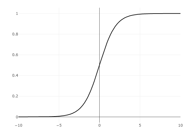
Logistic regression [5] is similar to linear regression except for that it is used to solve a classification problem. There are two core concepts in logistic regression, one is logit and the other is sigmoid function which is shown below.

The form of the logistic regression for the binary response variable $(y_{i})$ goes like

$$\log\frac{P(y_{i}=1|X=x_{i})}{1-P(y_{i}=1|X=x_{i})}=x_{i}\beta,\;\,\text{for}\;i=1,\ldots,n$$

where $x_{i}$ is a feature vector, $\beta$ is the coefficient vector with the intercept, $\frac{P(y_{i}=1|X=x_{i})}{1-P(y_{i}=1|X=x_{i})}$ is odds ratio, and $\log(\frac{P(y_i =1 | X = x_i)}{1-P(y_i = 1 | X = x_i)})$ is named logit. After transpositioning the terms in above equation, we can obtain the following formula.

$$P(y_{i}=1|X=x_{i})=\frac{e^{x_{i}\beta}}{1+e^{x_{i}\beta}}=\frac{1}{1+e^{-x_{i}\beta}},\;\,\text{for}\;i=1,\ldots,n$$

Now, it is obvious that the sigmoid function mentioned at first being used to model the probability of $y_{i}=1$. The coefficient vector $\beta$ is estimated by maximizing likelihood method given $y_{i}$ follows the bernoulli distribution. Moreover, we can transform the likelihood function by taking negative logarithm to obtain logloss (cross entropy). After calculating the partial derivative of logloss over $\beta$, the gradient descent takes into part to find the optimum of $\hat{\beta}$.

Learning Steps:

1. a.

   Update the logloss by numerical method such as gradient descent to obtain the optimal estimated coefficients.

2. b.

   Obtain

   	$\displaystyle\hat{p}_{new,\,c^{{}^{\prime}}}$	$\displaystyle=P(y_{new}=c^{{}^{\prime}}|X=x_{new})=\frac{1}{1+\sum_{k}e^{x_{new}\boldsymbol{\beta_{k}}}},\;\text{where}\;\,c^{{}^{\prime}}\;\,\text{is the pivot.}$
   	$\displaystyle\mathrlap{\hat{p}_{new,\,c}}\phantom{\hat{p}_{new,\,c^{{}^{\prime}}}}$	$\displaystyle=P(y_{new}=c\;|X=x_{new})=\frac{e^{x_{new}\boldsymbol{\beta_{c}}}}{1+\sum_{k}e^{x_{new}\boldsymbol{\beta_{k}}}},\;\,\text{for}\;\,c=1,\ldots,m\;\,\text{and}\;\,c\neq c^{{}^{\prime}}$

   and classify $x_{new}$ as

   $$\hat{y}_{new}=\arg\max_{c=1,\ldots,m}\{\hat{p}_{new,\,c}\}$$

As its name implies, random forest [6] is an ensemble learning method that operates by constructing a multitude of decision trees under random mechanism. A decision tree is drawn upside down with its root at the top. There are $3$ core elements in a decision tree which are internal node, edges, and external (leaf) node representing condition, branches, and decision, respectively. An external node is one without child branches, in contrast, internal node has at least one child branch. Below is a typical structure of a decision tree.

$A,B,C,E,G$ are internal nodes which are root node and $A,A,B,C$’s branches, respectively, and $D,H,I,F,J,K$ are external nodes. Note that the number of external nodes is exactly one more than the number of internal nodes.

Learning Steps:

1. a.

   Select a criterion, gini index or entropy, to measure the goodness of partition (feature + condition) in each internal nodes, where

   $$gini\;index=1-\sum^{m}_{c=1}P_{c}^{2}\in[0,\frac{m-1}{m}]$$

   and

   $$entropy=-\sum^{m}_{c=1}P_{c}\log_{2}(P_{c})\in[0,\log_{2}(m)]$$

   where $P_{c}$ is the proportion of records after a partition that belong to class $c$. In practice, the chosen of the impurity criterion does not influence testing performance much [7].

2. b.

   Tune the hyperparameters such as percentage of sample, percentage of features, maximum depth, etc, for constructing a tree with cross validation applied.

3. c.

   Drop a new record all the way down to an external node, we can assign its class simply by taking a “vote” of all the training data that belonged to that external node when the tree was grown [8]. Since there are several trees in random forest, we have to repeat the process and assign the class for that observation by “majority vote”.

4. d.

   Obtain

   $$\hat{p}_{new,\,c}=\hat{f}_{rf,\;c}(X=x_{new}),\;\,\text{for}\;c=1,\ldots,m$$

   and classify $x_{new}$ as

   $$\hat{y}_{new}=\arg\max_{c=1,\ldots,m}\{\hat{p}_{new,\,c}\}$$

Support vector machine [9] is composed of 4 core elements, the separating hyperplane, the maximum-margin concept, the type of margin (hard or soft-margin) and the kernel function. The goal of SVM is to find a hyperplane that can maximize the margin between two auxiliary hyperplanes being $l_{1}$ and $l_{3}$ in Figure 2.3, and the kernel function takes part in the situation that the original feature space is inseparable. Note that $l_{2}$ is the target hyperplane and it’s simply a line in the 2-dimensional case. $A,B,E,F$ are called support vectors since they support the construction of $l_{1}$ and $l_{3}$. The difference between soft and hard-margin is that whether the tolerance term $\xi$ (so-called slack variable) is included in the optimization, this slack variable is a trade-off term between the violation of hyperplane and the size of margin utilized in soft margin SVM. That is to say, the inclusion of $\xi$ in soft-margin SVM is used to solve the potential overfitting problem derived from hard-margin one. Below is the optimization problem that is tackled by soft-margin SVM.

$$\arg\min_{b,\;w,\;\xi}\frac{1}{2}w^{T}w+C\sum_{i=1}^{n}\xi_{i}$$

$$\text{subject to}\;\;y_{i}(\phi(x_{i})^{T}w+b)\geq 1-\xi_{i}$$

where $\xi_{i}\geq 0,\forall i=1,\ldots,n$, $C$ is a regularization hyperparameter and $\phi(\cdot)$ denotes the kernel trick.

XGBoost [10] is a boosting algorithm which is an ensemble method. It is a sequential one which combines several weak learners into a strong classifier. That is, it sequentially fits the residual from previous learner and produce a better one. The mathematical form of boosting concept is as follows.

$$\hat{y_{i}}^{(t)}=\sum_{k=1}^{t}f_{k}(x_{i})=\hat{y_{i}}^{(t-1)}+f_{t}(x_{i})$$

where $f_{k}$ is $k^{th}$ weak learner which can be either a tree or a linear model.

For further elaboration, let’s have a look on above Figure 2.4, where $A,B,\ldots,G$ are observations. This is a tree with $T=3$ and $q(A)=q(B)=1,q(C)=q(D)=2,$ etc. $w_{q(A)}=w_{q(B)}=0.16$ serving as an addition of previous prediction of $A$ and $B$. Therefore, $\Omega=3\gamma+\frac{1}{2}\lambda(0.0256+0.0144+0.01)$.

Now, we can replace $f_{t}(x_{i})$ and $\Omega(f_{t})$ in $L^{(t)}$ with their explicit forms. Let’s define a sample set $I_{j}=\{i\,|\,(q(x_{i})=j\}$ which is a collection of $i$ when $q(x_{i})$ equals to leaf $j$.

	$\displaystyle L^{(t)}$	$\displaystyle\approx\sum_{i=1}^{n}\left[g_{i}f_{t}(x_{i})+\frac{1}{2}h_{i}f_{t}^{2}(x_{i})\right]+\Omega(f_{t})$
		$\displaystyle=\sum_{i=1}^{n}\left[g_{i}w_{q(x_{i})}+\frac{1}{2}h_{i}w_{q(x_{i})}^{2}\right]+\gamma T+\frac{1}{2}\lambda\sum_{j=1}^{T}w_{j}^{2}$
		$\displaystyle=\sum_{j=1}^{T}\left[(\sum_{i\in I_{j}}g_{i})w_{j}+\frac{1}{2}(\sum_{i\in I_{j}}h_{i}+\lambda)w_{j}^{2}\right]+\gamma T$

For simplicity, let’s denote $G_{j}=\sum_{i\in I_{j}}g_{i}$ and $H_{j}=\sum_{i\in I_{j}}h_{i}$. Since every leaf node is independent to each other, thus $L^{(t)}$ reaches its minimum only when each leaf node reaches its minimum. Furthermore, $w_{j}$ is the only parameter unknown, the optimal $w_{j}$ with respect to $L^{(t)}$ can be obtained with the following method.

	$\displaystyle(\sum_{i\in I_{j}}g_{i})w_{j}+\frac{1}{2}(\sum_{i\in I_{j}}h_{i}+\lambda)w_{j}^{2}$	$\displaystyle=G_{j}w_{j}+\frac{1}{2}(H_{j}+\lambda)w_{j}^{2}$
		$\displaystyle=\frac{1}{2}(H_{j}+\lambda)(w_{j}+\frac{G_{j}}{H_{j}+\lambda})^{2}-\frac{1}{2}\frac{G_{j}^{2}}{H_{j}+\lambda}$

Hence, when $w_{j}=w_{j}^{*}=-\frac{G_{j}}{H_{j}+\lambda}$, the loss function is at its minimum with below form.

$$L^{(t)}\approx-\frac{1}{2}\sum_{i=1}^{T}\frac{G_{j}^{2}}{H_{j}+\lambda}+\gamma T$$

Now, we can define $Gain$ as a measurement for goodness of partition in XGBoost.

$$Gain=\frac{1}{2}\left[\frac{G_{L}^{2}}{H_{L}+\lambda}+\frac{G_{R}^{2}}{H_{R}+\lambda}-\frac{(G_{L}+G_{R})^{2}}{H_{L}+H_{R}+\lambda}\right]-\gamma$$

where subscript $L$ and $R$ denote the left and right node, respectively. By applying Greedy Algorithm, we can find the best combination of feature and value for each nodes in terms of $Gain$ until the pre-determined tree’s depth is met, then prune the nodes with negative gains.

Learning Steps:

1. a.

   Find the best combinations of hyperparameters utilized in XGBoost algorithm including max depth, $\gamma$, $\lambda$, number of trees (estimators), min child weight, percentage of features, etc with the cross validation applied.

2. b.

   Drop a new record all the way down to an external node for all estimators. Calculate the total of the initial prediction and all the corresponding outputs ($w_{j}$) at external nodes, then set a threshold value to classify the new record. Note that for multi-class classification problem, we’ll build $n$ estimators for each class and transform the predictions with softmax function to produce probabilities.

3. c.

   Obtain

   $$\hat{p}_{new,\,c}=\hat{f}_{xgb,\;c}(X=x_{new}),\;\,\text{for}\;c=1,\ldots,m$$

   and classify $x_{new}$ as

   $$\hat{y}_{new}=\arg\max_{c=1,\ldots,m}\{\hat{p}_{new,\,c}\}$$

A neural network [11] consists of several layers and each layer is made of several units which are known as neurons. Below is the figure of a typical fully connected ANN, which is also named as fully connected feedforward neural network.

The input $\{x_{l}\}_{l=1,\ldots,n}$ is transmitted from the input layer to the hidden layer. The hidden layer activates the weighted input and output the activated value. The output layer receives the weighted input from hidden layer and activates again to obtain the final $\hat{y}_{l}$. Each line in the above figure represents a weight $w_{ij}$ being a multiplier of the corresponding neuron, output layer can be obtained from the following equation (note that Figure 2.5 is drawn under $m=3$).

$$p_{lc}(x_{l})=\sigma_{hidden}(b^{\prime}_{c}+\sum^{n_{hidden}}_{j=1}w^{\prime}_{jc}z_{lj}(\sigma_{input}(b_{j}+\sum^{n_{input}}_{i=1}w_{ij}x_{li})),\;\text{where}\;c=1,\ldots,m$$

where $\sigma(\cdot)$ is a non-linear activation function such as the sigmoid function, softmax function, or rectified linear unit and $w,w^{\prime},b,b^{\prime}$ are the parameters needed to be estimated. As for how to learn parameters, a loss function has to be specified, we then update the parameters by conducting optimization procedure such as gradient descent to find the optimal parameter combinations.

Learning Steps:

1. a.

   Build network structure (determine the number of layers, the number of neurons in each layers, and the type of activation functions for each layers).

2. b.

   Specify a loss function, typically, the cross entropy loss is applied for classification problem. It has the following form.

   $$L=-\sum^{m}_{c=1}\sum^{n}_{l=1}y_{lc}\log_{2}(p_{lc})$$

3. c.

   Update weights $W$ and biases $B$ through gradient descent algorithm with backpropagation applied. Note that a suitable learning rate for training is critical to minimize the loss.

4. d.

   Obtain

   $$\hat{p}_{new,\,c}=\hat{f}_{nn,\;c}(X=x_{new}|W^{*},B^{*}),\;\,\text{for}\;c=1,\ldots,m$$

   and classify $x_{new}$ as

   $$\hat{y}_{new}=\arg\max_{c=1,\ldots,m}\{\hat{p}_{new,\,c}\}$$

Let $\Omega\subset{\hbox{I\kern-1.99997ptR}}^{p}$ be a collection of observations which is composed of elements of $m$ different memberships. The memberships are labeled as $1,\ldots,m$. A part of observations $\Omega_{\rm tr}\subset\Omega$, typically called training set, and another part of observations $\Omega_{\rm tt}\subset\Omega$, typically called test set, are prepared from $\Omega$. It is assumed that $\Omega_{{tr}}$ and $\Omega_{{tt}}$ are sufficiently large and these two sets share the same characteristics represented by the whole data space $\Omega$.

After previous elaboration of QMS structure, let’s have a look on its schematic diagram. This diagram is constructed under the settings of $p=4,q=2,m=3$ meaning that the dataset is $4$-dimensional with $3$ labels, $A_{i}$ contains $4\times 2$ parameters, and $b_{i}$ contains $2$ parameters.

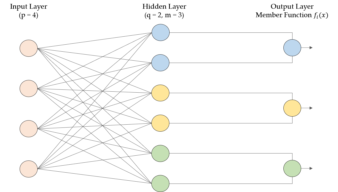
Each line extending from the input layer indicates a weight $a^{(i)}_{jk}$ in $A_{i}$, where $i\in M,j=1,\ldots q,k=1,\ldots,p$, thus, we can see there are $24$ lines equalling to $pqm=4\times 2\times 3$. Note that the weights in $b_{i}$ are not shown in the diagram. Furthermore, the straight lines connect to the output layer indicating a sum of squares operation which allows us to obtain the member function $f_{i}(x)$ for all $i\in M$. Therefore, it is clear that the number of parameters in QMS is controlled by $p,q,m$, and $q$ is the only hyperparameter that can be specified manually.

We propose to train QMS / update the weights of QMS via gradient descent with the technique of Adam[12] applied. Let’s recall the form of loss function $\Phi$.

	$\displaystyle\Phi(f_{1},\ldots,f_{m})$	$\displaystyle=\sum_{j=1}^{m}\left\{\sum_{x\in\,\Omega_{tr}(j)}\sum_{k\in M,\,k\neq j}\max\left\{\alpha_{jk},\frac{f_{j}(x)}{f_{k}(x)}\right\}\right\}$
		$\displaystyle=\sum_{j=1}^{m}\left\{\sum_{x\in\,\Omega_{tr}(j)}\sum_{k\in M,\,k\neq j}\max\left\{\alpha_{jk},\frac{\lVert A_{j}x-b_{j}\rVert^{2}}{\lVert A_{k}x-b_{k}\rVert^{2}}\right\}\right\}$

where $f_{i}(x)=\lVert A_{i}x-b_{i}\rVert^{2}$, $A_{i}\in{\hbox{I\kern-1.99997ptR}}^{q\times p},b_{i}\in{\hbox{I\kern-1.99997ptR}}^{q},x\in{\hbox{I\kern-1.99997ptR}}^{p}$ for all $i\in M$, $q$ is a hyperparameter, $p$ denotes the number of attributes, and $m$ denotes the number of classes, where $p$ and $m$ are predetermined by data. Our goal is to find a classifier with the best combinations of $\{A_{i},b_{i}\}_{i\in M}$ by minimizing $\Phi(f_{1},\ldots,f_{m})$. Below we demonstrate a simple case for above equation under $m=2$ to get insights of it.

	$\displaystyle\Phi(f_{1},f_{2})$	$\displaystyle=\sum_{x\in\Omega_{tr}(1)}\max\left\{\alpha_{12},\frac{f_{1}(x)}{f_{2}(x)}\right\}+\sum_{x\in\Omega_{tr}(2)}\max\left\{\alpha_{21},\frac{f_{2}(x)}{f_{1}(x)}\right\}$
		$\displaystyle=\sum_{x\in\Omega_{tr}(1)}\max\left\{\alpha_{12},\frac{\lVert A_{1}x-b_{1}\rVert^{2}}{\lVert A_{2}x-b_{2}\rVert^{2}}\right\}+\sum_{x\in\Omega_{tr}(2)}\max\left\{\alpha_{21},\frac{\lVert A_{2}x-b_{2}\rVert^{2}}{\lVert A_{1}x-b_{1}\rVert^{2}}\right\}$

As we can find from above example, $A_{1},A_{2},b_{1}$ and $b_{2}$ are the parameter matrices required to be updated. Thus, it is clear that the total number of parameter matrices is $m\times 2$ with the actual number of parameters $qm(p+1)$ which can be derived from the following formula.

$$\text{number of parameters}=qpm+qm=qm(p+1)$$

Therefore, under the case of $m=2$, there are $4$ parameter matrices with $2q(p+1)$ total parameters. After revealing the unknown parameters in QMS-specific loss function, it’s time to deep dive into the mathematical derivation and the training algorithm of QMS.