Over-Conservativeness of Variance-Based Efficiency Criteria and Probabilistic Efficiency in Rare-Event Simulation

To motivate the various notions that we would discuss momentarily, let us consider using crude Monte Carlo to estimate $p$. This means we utilize the unbiased estimator $Z=I_{\mathcal{A}_{\gamma}}$ for $p$, where $I_{\mathcal{A}_{\gamma}}$ denotes the indicator variable on the event $\mathcal{A}_{\gamma}$. Suppose we generate the output $Z$ independently $n$ times, and construct $\hat{p}$ as their sample mean. Intuitively, when $p$ is tiny, this estimator $\hat{p}$ is most likely zero unless $n$ is a huge number, since a long trial length is needed to land at the rare event $\mathcal{A}_{\gamma}$.

To describe the above challenge mathematically, we consider the following criterion. For a given tolerance level $\varepsilon>0$ (e.g., $5\%$), we would like an estimator $\hat{p}$ to satisfy

for a certain $0<\delta<1$ when using a simulation size $n$. In (1), the closeness between $\hat{p}$ and $p$, which represents the error of $\hat{p}$ in estimating $p$, is measured relative to the magnitude of $p$ itself. This is because for tiny $p$, the estimation is only meaningful if the error is small enough relative to this tiny quantity. Linking to crude Monte Carlo, outputting merely $\hat{p}=0$, as likely to happen thereby, would be viewed as incurring a substantial error, i.e., lying in the event $|\hat{p}-p|>\delta p$ in (1). Put in another way, we argue that a huge sample size $n$ is needed for crude Monte Carlo to attain (1). Note that by Chebyshev’s inequality, we get that for any $0<\delta<1$,

Hence, $n\geq\frac{Var(Z)}{\varepsilon\delta^{2}p^{2}}$ implies that $P(|\hat{p}-p|>\delta p)\leq\varepsilon$ for $\varepsilon>0$. This means that $\frac{Var(Z)}{\varepsilon\delta^{2}p^{2}}$ is a sufficient size for $n$ to achieve (1). This quantity depends on the ratio between the standard deviation $\sqrt{Var(Z)}$ and the mean $p$, which is known as the relative error. Here, for crude Monte Carlo the relative error is $\frac{\sqrt{Var(Z)}}{p}=\frac{\sqrt{p(1-p)}}{p}=\sqrt{\frac{1-p}{p}}$ which blows up as $p\to 0$. Consequently, the sufficient size for $n$ also blows up as $p\to 0$. In particular, if $p$ decays exponentially in $\gamma$ – a typical scaling in large deviations, then the required $n$ to achieve (1) also scales exponentially.

The above challenge motivates variance reduction techniques to reduce the sample size requirement. Among the most popular is IS. In this approach, we generate samples from an alternate measure $\tilde{P}$ where $\tilde{P}$ satisfies $PI_{\mathcal{A}_{\gamma}}\ll\tilde{P}$ (i.e., $PI_{\mathcal{A}_{\gamma}}$ is absolutely continuous with respect to $\tilde{P}$), and use $Z=I_{\mathcal{A}_{\gamma}}\frac{dP}{d\tilde{P}}$ as an unbiased output for $p$, where $\frac{dP}{d\tilde{P}}$ is the Radon-Nikodym derivative, or the so-called likelihood ratio, between $P$ and $\tilde{P}$. Though this output is always unbiased thanks to the likelihood ratio adjustment, the performance of the IS estimator in terms of variability heavily depends on the choice of the IS probability measure $\tilde{P}$. In the literature, several efficiency criteria for IS estimators have been developed. A common criterion is asymptotic efficiency (Asmussen and Glynn 2007, Heidelberger 1995, Juneja and Shahabuddin 2006):

For functions $f,g:\mathbb{R}\to\mathbb{R}$, we say $g(\gamma)$ is subexponential in $f(\gamma)$ as $\gamma\to\infty$ if $\lim_{\gamma\to\infty}\frac{\log g(\gamma)}{f(\gamma)}=0$, i.e. $g(\gamma)=\exp(f(\gamma)o(1))$. For functions $f,g,h$, clearly if $\lim_{\gamma\to\infty}\frac{\log g(\gamma)}{f(\gamma)}=\lim_{\gamma\to\infty}\frac{\log h(\gamma)}{f(\gamma)}$, then $\lim_{\gamma\to\infty}\frac{\log(g(\gamma)/h(\gamma))}{f(\gamma)}=0$ and hence $g(\gamma)/h(\gamma)$ is subexponential in $f(\gamma)$ as $\gamma\to\infty$. By taking $g(\gamma)=\tilde{E}(Z^{2})$, $h(\gamma)=p^{2}$ and $f(\gamma)=\log p$, we see that the condition in Definition 2.1 is equivalent to the condition that $\tilde{E}(Z^{2})/p^{2}$ (or $\widetilde{Var}(Z)/p^{2}$) is subexponential in $-\log p$ as $\gamma\to\infty$.

From (2) and its subsequent discussion, asymptotic efficiency implies that the required simulation size $n$ to attain a prefixed relative error grows only subexponentially in $-\log p$. As a stronger requirement, $Z$ is said to have a bounded relative error if $\limsup_{\gamma\to\infty}\frac{\widetilde{Var}(Z)}{p^{2}}<\infty$, which implies that the required simulation size remains bounded no matter how small $p$ is. The criterion of bounded relative error is sometimes too strict to achieve, so we focus on asymptotic efficiency in this paper. More efficiency criteria could be found in Juneja and Shahabuddin 2006, L’Ecuyer et al. 2010, Blanchet and Lam 2012.

In the large deviations setting, the classical notion of dominating points is used to guarantee asymptotic efficiency of IS (Sadowsky and Bucklew 1990). To explain, let us first recall the so-called rate function in the large deviations theory which, intuitively speaking, measures the likelihood of hitting each point on an exponential scale. More specifically, we consider the standard Gartner-Ellis regime as follows (Dembo and Zeitouni 2009, Bucklew 2004). Without loss of generality consider $\gamma>0$. Suppose that $\mathcal{A}_{\gamma}=\{\frac{1}{\gamma}X_{\gamma}\in\mathcal{E}\}$ where $\{X_{\gamma}\}_{\gamma}$ are $\mathbb{R}^{d}$-valued random variables and $\mathcal{E}$ is a fixed Borel set in $\mathbb{R}^{d}$. We define $\mu_{\gamma}(x)=\frac{1}{\gamma}\log E(e^{x^{\top}X_{\gamma}}),x\in\mathbb{R}^{d}$ as the scaled logarithmic moment generating function. We denote $\mathcal{D}(f)=\{x:f(x)<\infty\}$ as the domain of a function $f$. With these, we assume the following: {assumption} $\mu_{\gamma}(x)$ satisfies the following conditions:

1. 1.

   $\mu(x)=\lim_{\gamma\to\infty}\mu_{\gamma}(x)$ exists for any $x\in\mathbb{R}^{d}$, where we allow $\infty$ both as a limit value and as an element of the sequence $\{\mu_{\gamma}(x)\}$;

2. 2.

   $0\in\mathcal{D}(\mu)^{\circ}$;

3. 3.

   $\mu$ is essentially smooth, i.e., $\mathcal{D}(\mu)^{\circ}$ is non-empty, $\mu$ is differentiable everywhere in $\mathcal{D}(\mu)^{\circ}$ and $\mu$ is steep.

Then we define the rate function $I(y)=\sup_{x\in\mathbb{R}^{d}}\{x^{\top}y-\mu(x)\},y\in\mathbb{R}^{d}$ as the Legendre transform of $\mu$. For any set $\mathcal{E}\subset\mathbb{R}^{d}$, we denote $I(\mathcal{E})=\inf_{y\in\mathcal{E}}I(y)$. We make the following assumptions for the set $\mathcal{E}$: {assumption} $\mathcal{E}\subset\mathbb{R}^{d}$ is a Borel set such that $\overline{\mathcal{E}}=\overline{\mathcal{E}^{\circ}}$, $\mathcal{E}^{\circ}\cap\mathcal{D}(I)^{\circ}\neq\emptyset$ and $I(\mathcal{E})>0$.

Under these assumptions, we have the following result (e.g., adapted from Dembo and Zeitouni 2009 Theorem 4.5.3.6):

Assumptions 2.3 and 2.3 are standard light-tailed conditions on $\mathcal{A}_{\gamma}$, which guarantee the considered probability $P(\mathcal{A}_{\gamma})$ to decay exponentially in $\gamma$ with decay rate $I(\mathcal{E})$. The rate function $I(y)$ can be viewed as a measurement on the likelihood of hitting $y$ in the exponential scale. The most likely point to hit among $\mathcal{E}$ is hence given by the minimizer of $I(y)$ over $\mathcal{E}$, resulting in the overall exponential decay rate $I(\mathcal{E})$. Note that, by Theorem 2.2, we have $-\log p=\Theta(\gamma)$ as $\gamma\to\infty$, and hence subexponential (or exponential) in $-\log p$ is equivalent to subexponential (or exponential) in $\gamma$.

Now we present the concept of dominating points and sets:

Dominating points can be understood as the “local minimizers” of the rate function $I$ in the sense that $a_{i}$ is the minimizer of $I$ in $\mathcal{E}\cap\{x\in\mathbb{R}^{d}:s_{a_{i}}^{\top}(x-a_{i})\geq 0\}$. To understand this, first, Condition 1 in Definition 2.3 stipulates that $s_{a_{i}}$ is the gradient of $I(x)$ at the point $a_{i}$. Then, in Condition 2, $a_{i}$ can be seen as the minimizer of $I(x)$ over the set $\{x\in\mathbb{R}^{d}:s_{a_{i}}^{\top}(x-a_{i})\geq 0\}$, a fact that follows from the first-order optimality condition in convex function minimization. Thus, Condition 2 stipulates that any point in the rare-event set $\mathcal{E}$ has an $I$ value not less than one of the $a_{i}$’s. Geometrically, any points in the set $\mathcal{E}$ must lie in the half-space tangentially cut by one of the $a_{i}$’s (i.e., the “backyard” of the $a_{i}$). Figure 1 is an illustration of a rare-event set $\mathcal{E}=\mathcal{E}_{1}\cup\mathcal{E}_{2}$ and the dominating set $\{a_{1},a_{2}\}$. Here, $a_{1}$ is the global minimum rate point in $\mathcal{E}$, but $\mathcal{E}_{2}$ is not covered by $\{x:s_{a_{1}}^{\top}(x-a_{1})\geq 0\}$, so $a_{2}$ is included in the dominating set. Finally, we note that Condition 3 in Definition 2.3 enforces the dominating set to be the minimal set of points such that the geometric properties in Conditions 1 and 2 are satisfied.

Note that dominating points may not be local minimizers of the rate function $I$ in $\mathcal{E}$ (even though they are minimizers in $\mathcal{E}\cap\{x\in\mathbb{R}^{d}:s_{a_{i}}^{\top}(x-a_{i})\geq 0\}$ as discussed above). Nonetheless, the most significant dominating points are indeed global minimizers of $I$ in $\mathcal{E}$. This is presented in the following theorem:

We should also point out that dominating set defined according to Definition 2.3 may not be unique. Advantageously, the theory and estimators we present will flexibly apply to any such dominating set.

We are now ready to describe the main message of this section, which is the established recipe in constructing efficient IS. The standard proposal is to use a mixture of exponentially tilted distributions, where each exponential tilting is with respect to each dominating point. In particular, suppose that $A=\{a_{1},\dots,a_{r}\}$ is a dominating set. Then the IS distribution is $\tilde{P}$ such that

with $\sum_{i=1}^{r}\alpha_{i}=1,\alpha_{i}>0,\forall i$. Here, $e^{s_{a_{i}}^{\top}X_{\gamma}-\gamma\mu_{\gamma}(s_{a_{i}})}dP$ is the exponential tilting towards the dominating point $a_{i}$ and $\alpha_{i}$’s are the mixing weights. The IS (3) is well known to be asymptotically efficient:

While the proof of Proposition 2.5 is standard, we include it in the Appendix for self-containedness. Here, we describe the key intuition in justifying the necessity of mixture. First, the likelihood ratio in the considered mixture IS is

and it satisfies that for any $i$,

In the exponent in the rightmost expression of (4), the second term $\gamma(s_{a_{i}}^{\top}a_{i}-\mu_{\gamma}(s_{a_{i}}))$ is approximately $\gamma I(a_{i})$, and the first term is the “overshoot” of the sampled $X_{\gamma}$ compared to the dominating point $a_{i}$. That is, if $X_{\gamma}$ is in the “backyard” of $a_{i}$, then this term $s_{a_{i}}^{\top}(X_{\gamma}-\gamma a_{i})\geq 0$. The definition of dominating set, especially Condition 2 in Definition 2.3, guarantees any $(1/\gamma)X_{\gamma}$ in $\mathcal{E}$ must have $s_{a_{i}}^{\top}(X_{\gamma}-\gamma a_{i})\geq 0$ for at least one of the $i$’s. Thus, by decomposing the second moment of $Z=I_{\mathcal{A}_{\gamma}}L$ according to the backyards of $a_{i}$’s, we can ensure that the magnitude of the likelihood ratio, when $X_{\gamma}$ lies inside the rare event set, is properly controlled. More precisely, write $\mathcal{E}=\bigcup_{i=1}^{r}\mathcal{E}_{i}$ where each $\mathcal{E}_{i}\subset\{x:s_{a_{i}}^{\top}(x-a_{i})\geq 0\}$. Then the second moment of the IS satisfies

which is approximately bounded by $\sum_{i=1}^{r}e^{-2\gamma I(a_{i})}/\alpha_{i}^{2}$ and hence $e^{-2\gamma I(\mathcal{E})}$ in the exponential scale, thus verifying asymptotic efficiency.

On the other hand, if we miss some dominating points in the construction of the mixture IS, then asymptotic efficiency may fail to be attained. Below we give a simple example to demonstrate this.

In this example, the dominating points are $1$ and $-2$, and $N(\gamma,\gamma)$ is the exponential tilt towards the first dominating point $1$ (for Gaussian distribution, exponential tilting amounts to a mean shift). Here, by considering only this point, it is possible that a generated $X_{\gamma}$ satisfies $(1/\gamma)X_{\gamma}\in(-\infty,-2]$ while the overshoot $s_{1}^{\top}(X_{\gamma}-\gamma 1)$, as explained for (4), takes a very negative value. This scenario contributes significantly to the overall variance and ultimately violates asymptotic efficiency.

Our main insight in this paper is a rebuke of the above viewpoint. More specifically, we argue that missing inferior dominating point, such as the example in Proposition 2.6, can still result in a good IS according to our beginning criterion (1). A core ingredient of this assertion is to question the use of asymptotic efficiency, or more generally variance-based efficiency criteria. Before delving into the theory, let us first present some numerical results to shed light on how much difference it makes to use different numbers of dominating points in the IS mixture. This is the focus of our next section.

We consider the problem of estimating the tail probability involving a sum of random variables, where $Y_{1},Y_{2},...$ are i.i.d and we are interested in

where $S_{m}=\sum_{i=1}^{m}Y_{i}$. We consider $m$ as the rarity parameter $\gamma$ presented in Section 2. Using the notation in the Gartner-Ellis regime, we have $X_{\gamma}=S_{m}$ and $\mathcal{E}=(-\infty,-a]\cup[a,\infty)$. Then $\mu(x)=\log E(e^{xY_{1}})$ and we suppose Assumption 2.3 is satisfied. By Theorem 2.2, when $|EY_{1}|<a$, if $s_{a}$ and $s_{-a}$ satisfy $\nabla\mu(s_{a})=a$ and $\nabla\mu(s_{-a})=-a$, then we have

and

For this problem, Glasserman and Wang 1997 Section 3 provides two estimators, $\hat{\alpha}(m)$ and $\hat{\beta}(m)$. Specifically, we have $\hat{\alpha}(m)=\exp(-s_{a}S_{m}+m\mu(s_{a}))I_{\{|S_{m}|\geq am\}}$ with samples of $Y_{i}$ generated from exponentially tilted distribution using $s_{a}$. The estimator $\hat{\beta}(m)=\exp(-s_{a}S_{m}+m\mu(s_{a}))I_{\{S_{m}\geq am\}}+\exp(-s_{-a}S_{m}^{\prime}+m\mu(s_{-a}))I_{\{S_{m}^{\prime}\leq-am\}}$ with $S_{m}$ and $S_{m}^{\prime}$ constructed from independent sequences of i.i.d. $Y_{i}$’s and $Y_{i}^{\prime}$’s generated from exponentially tilted distributions using $s_{a}$ and and $s_{-a}$ respectively. That is, $\hat{\beta}(m)$ attempts to estimate $P(S_{m}\geq am)$ and $P(S_{m}\leq-am)$ separately using different IS samples and sum up these estimates. Here, $\hat{\alpha}(m)$ only uses one dominating point whereas $\hat{\beta}(m)$ uses both points (note that even though $\hat{\beta}(m)$ does not use the mixture IS scheme in (3), the idea is similar in that it accounts for both dominating points). In our experiment, we follow Glasserman and Wang 1997 to set $Y_{1}=A-B$ with $A\sim N(1.5,1)$, $B\sim Exp(1)$ and $A,B$ independent, and $a=1.5$ (in this case, $s_{a}=(\sqrt{5}-1)/2$, $s_{-a}=-2+\sqrt{2}$, and $I(a)\approx 0.2902$, $I(-a)\approx 0.7044$).

We run numerical experiments with $m=10$, $30$, $50$ and $100$. The results using $10^{4}$ samples are shown in Table 1. By comparing the numbers in the second and third rows, we observe that $\hat{\alpha}(m)$ and $\hat{\beta}(m)$ have very similar empirical performances. However, note that:

In view of Proposition 3.1, $\hat{\alpha}(m)$ is arguably a very poor estimator as it bears an exploding variance. We therefore see an apparent discrepancy between empirical performances and theoretical guidance – The theoretically bad variance does not result in poor empirical performances. Proposition 3.1 is proved in Glasserman and Wang 1997, where the asymptotic efficiency of $\hat{\beta}(m)$ follows from their Proposition 1, while the variance behavior of $\hat{\alpha}(m)$ appears in their Theorem 1.

We consider the problem of estimating the overshoot probability of the finite-horizon maximum of a random walk. We define the probability of interest as

where $S_{m}=\sum_{i=1}^{m}Y_{i}$ and $Y_{i}$’s are Gaussian distributed with mean 0, standard deviation $\sigma$, and pairwise correlation $-0.02$, i.e., $corr(Y_{i},Y_{j})=-0.02$ for any $i,j\in\{1,...,d\}$ with $i\neq j$. Suppose that the rarity parameter is $\gamma=1/\sigma^{2}\to\infty$. We note that we can reformulate this target rare event as $\left\{\frac{1}{\gamma}X_{\gamma}\in\bigcup_{m=1}^{d}\mathcal{H}_{m}\right\}$ where $X_{\gamma}=\gamma(Y_{1},\dots,Y_{d})^{\top}$ and $\mathcal{H}_{m}=\{x\in\mathbb{R}^{d}:\sum_{i=1}^{m}x_{i}\geq a\}$ with $x_{i}$ denoting the $i$th element in $x$. This decomposition allows us to construct an IS estimator using the $d$ dominating points corresponding to each half-space $\mathcal{H}_{m}$. More specifically, in this example, $I(y)=\frac{1}{2}y^{\top}\Sigma^{-1}y$, and the dominating points, ranking from the most to the least significant (i.e., increasing rate function value), are $a_{1}=\frac{a\Sigma e_{d}}{e_{d}^{\top}\Sigma e_{d}},a_{2}=\frac{a\Sigma e_{d-1}}{e_{d-1}^{\top}\Sigma e_{d-1}},\dots,a_{d}=\frac{a\Sigma e_{1}}{e_{1}^{\top}\Sigma e_{1}}$, where $e_{i}$ denotes the vector with 1 in the first $i$ elements and 0 for the rest.

In our experiments, we fix $a$ and vary $\sigma$ for different rarity levels. In addition, we set $d=10$. We generate $10^{4}$ samples from IS distributions using a varying, partial list of dominating points. That is, we choose the IS distributions for $X_{\gamma}$ as $\frac{1}{k}\sum_{i=1}^{k}\phi(x;\gamma a_{i},\gamma\Sigma)$, where $\phi(x;a,b)$ denotes the Gaussian density with mean $a$ and variance $b$, for $k=1,\dots,d$. The performances of these IS estimators are shown in Table 2. We observe that these estimators with different numbers of dominating points all perform similarly. In particular, we present the cases with $\sigma=0.2$ and $\sigma=0.3$ respectively in Figure 2. We observe that in both cases the performances of the IS estimators are almost independent of the number of used dominating points, with the probability estimates all comparable while using more dominating points slightly increases the CI width.

On the other hand, Proposition 2.5 implies that the IS using all dominating points is asymptotically efficient while we have:

Thus, like in Section 3.1, there appears a mismatch between theoretical guidance and empirical observation. The asymptotic inefficiency of simple exponential tilting towards only the most significant dominating point does not result in a poor experimental performance.

We consider a rare-event probability estimation problem from an image classification task. Our goal is to estimate the probability of misclassification when the input of a prediction model is perturbed by tiny noise. This probability estimate is of interest as a robustness measure of the prediction model (Webb et al. 2018). More specifically, suppose that the prediction model $g$ is able to predict the label of input $x_{0}$, i.e. $g(x_{0})=c$ where $c$ is the true label of $x_{0}$. Then $P(g(x_{0}+\varepsilon)\neq c)$ where $\varepsilon$ is a random perturbation can be used to measure the robustness of $g$.

In particular, we consider the classification problem on MNIST dataset which contains 70,000 images of handwritten digits and each image consists of $28\times 28$ pixels. We train a 2-ReLU-layer neural network with 20 neurons in each layer using 60,000 training data, which achieves approximately 95% of testing data accuracy in predicting the digits. We perturb a fixed input (that is correctly predicted) with a Gaussian noise with mean 0 and standard deviation $\sigma$ on each of the 784 dimensions to assess the robustness of the prediction. Note that the rarity of this problem is determined by the value of $\sigma$, and we let the rarity parameter $\gamma=1/\sigma^{2}\to\infty$. The target rare event can be reformulated as $\left\{\frac{1}{\gamma}X_{\gamma}\in\{x:g(x_{0}+x)\neq c)\}\right\}$ where $X_{\gamma}=\gamma\varepsilon$.

We apply mixtures of exponential tiltings as IS estimators for this problem, namely by considering the IS distribution $\frac{1}{k}\sum_{i=1}^{k}\phi(x;\gamma a_{i},\gamma I)$, where $\phi(x;a,b)$ denotes the Gaussian density with mean $a$ and variance $b$ as in Section 3.2, for $k=1,2,\ldots$. Here $a_{i},i=1,2,\ldots$ denote the dominating points. In order to compute these points, we apply the scheme introduced in Huang et al. 2018 and Bai et al. 2022, which sequentially searches for dominating points by minimizing the rate function on the rare-event set that excludes the half-spaces cut from previous more significant dominating points. In the Gaussian case with piecewise linear rare-event set boundary as in our current example, each iteration amounts to finding the highest-density point on a piecewise-linear-boundary set, which can be conducted using mixed integer programming (see Algorithm 1 in the Appendix). Due to the high dimensionality of the input space and the complexity of the neural network predictor, the number of dominating points in this problem is huge. We implemented this sequential searching algorithm and it took a week to find the first 100 dominating points. Since we stopped the algorithm prematurely, the actual number of dominating points can be much larger. We run IS distributions with different numbers of dominating points (ranging from 1 to 41) and magnitudes of $\sigma$ (ranging from $0.1$ to $0.2$) and report the estimated probabilities and CIs. We use $10^{5}$ samples for IS estimators and $10^{7}$ samples for crude Monte Carlo estimators.

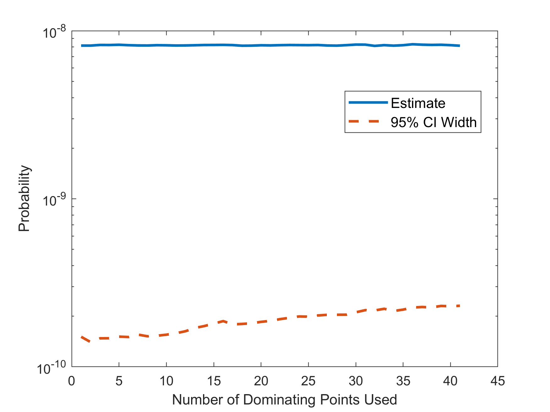
Figures  and show the results. Missing less significant dominating points does not seem to make noticeable differences in this problem. As shown in Figure , when we fix the rarity of the problem, the estimate is not sensitive to the number of dominating points. The CI width has an increasing trend as the number of dominating points gets larger, indicating that additional dominating points can in fact even hurt performances.

In Figure , we vary the rarity of the problem and compare the performances of different IS estimators and crude Monte Carlo. Note that estimates using crude Monte Carlo are unavailable for rarer configurations due to its inefficiency. We observe that the estimates from different IS estimators overlap visually in all considered cases, which indicates that the differences among these estimates are negligible. We also note that these estimates are consistent with the crude Monte Carlo estimates (when available), which shows their correctness.

Nonetheless, once again we have an apparent mismatch between theoretical inefficiency and good empirical performances: