Contact Information Flow and Design of Compliance

Let the robot and environment be described by generalized position $q\in Q=\mathbb{R}^{D}$ with velocity $\dot{q}$. Compliance (in the joint, gripper, or environment) can then be modelled by adding to the standard manipulator equations of motion as [30]

where $M(q)\in\mathbb{R}^{D\times D}$ is the inertia matrix, $\tau(q,\dot{q})\in\mathbb{R}^{D}$ contains the gravitational, Coriolis, and friction forces, spring-like forces $K:\mathbb{R}^{D}\rightarrow\mathbb{R}^{D}$, and input matrix $B(q)\in\mathbb{R}^{D\times K}$ modifies motor torque input $\tau_{m}\in\mathbb{R}^{K}$.

This model will be reduced to a two-mass model in the direction of contact motion, but provides the general statement for contact state and observations.

Contact is modelled as an equality constraint over total configuration, $\phi(q)=0$ [3]. A compliant contact model is used here [5, 4] instead of impulse-based [3] – it is assumed that sufficient compliance is present that collision forces can be represented as a function over configuration $q$.

While inequality constraints $\phi(q)\geq 0$ can capture non-penetration constraints, thereby modelling both free-space and constrained dynamics in a unified way [6], the approach here instead uses a collection of equality constraints, only one of which is active at once. Therefore, the contact state is then a discrete variable $n\in[1,\dots,N]$, where each contact state $n$ has a corresponding constraint $\phi_{n}(q)=0$.

Denote a position measurement at time step $t$ which measures some of the robot/environment positions $\theta_{t}\in\Theta\subset Q$, representing, e.g. that motor positions are measured, but the position of links or environmental inertias are not.

Let the measured torques/forces $f_{t}\in\mathbb{R}^{L}$ be a subset of the forces on compliant elements,

where ${\bf\epsilon}_{t}\sim\mathcal{N}(0,\Sigma_{f})$ is i.i.d. noise capturing electrical or quantisation noise, and $K^{n}_{f}:Q\rightarrow\mathbb{R}^{L}$ the effective sensor stiffness for the mode $n$. Therefore

As force/torque sensors measure displacement - either strain or bulk displacement [31] - practical force measurements can be described with (2).

When the system is fully observed, i.e. $\Theta=Q$, a prior belief $p({n})$ is updated by a measurement $f,\,\theta$ as

where the denominator is a normalization constant.

In the fully observed case, multiple measurements are independent as $\epsilon_{t}$ in (2) is i.i.d., and the full posterior is

This can be updated recursively as a hidden Markov model [32].

In the partially observed case, some positions are not directly measured. This can arise from joint flexibility (motor position is measured, link position is not), or from inertia in the environment. In this case, there are force contributions from the unmeasured inertias which will appear with the forces resulting from the contact mode.

We denote measured position $\theta_{t}$ and unmeasured position $\overline{q}_{t}$, so $q_{t}=[\theta_{t}^{T},\overline{q}_{t}^{T}]^{T}$, making the force observation model $p(f_{t}|\overline{q}_{t},\theta_{t},n)$. A dynamic model such as a discretized version of (1) can be used for inference, where we assume the dynamics $p(\overline{q}_{t+1}|n,\overline{q}_{t},\theta_{t})$ are known (these are derived for linear inertial system in Section 4.2). With these dynamics, a standard recursive estimate can be written [32, Ch. 2.4]

where $p(\overline{q}_{1})$ is a distribution of initial position ${\bf\overline{q}}_{1}$. To calculate (6), a Kalman filter can be used in the linear case [32, Ch. 3.2], and in the nonlinear flexible-joint robot case, various observers of link-side position/velocity are established [33].

The observation model (3) then needs to be marginalized over ${\bf\overline{q}}_{t}$ as

We assume the force observations (2) are linear, i.e. $K^{n}_{f}(q_{t})=K^{n}_{f}(q_{t}-q_{0}^{n})$ where $K^{n}_{f}\in\mathbb{R}^{L\times D}$ and $q_{0}^{n}$ is the rest position of the spring. Denote the posterior belief of $p(q_{t}|n,f_{1:t-1},\theta_{1:t-1})=\mathcal{N}(\mu^{n}_{q},\Sigma^{n}_{q})$, then the force measurement is distributed as

Note that the covariance in ${\bf f}_{t}$ now depends on the uncertainty in the position $\Sigma_{q}^{n}$, the stiffness $K_{f}^{n}$, and force sensor noise $\Sigma_{f}$.

The information gain is proposed as the reduction in uncertainty from $p(n)$ to $p(n|f,\theta)$, i.e. how much a measurement reduces belief entropy. Recall that entropy measures the uncertainty of a discrete random variable $H({\bf n})=-\sum_{n=1}^{N}p(n)\ln(p(n))$ and differential entropy over continuous random variables $h({\bf x})=-\int p(x)\ln p(x)dx$ [34, Ch. 2], we define the information gain as

A larger $\Delta_{I}$ means that the measurement brings more certainty.

Denoting a belief vector $b\in\mathbb{R}^{N}$, where $p(n=m)=b_{m}$, $b_{m}>0$, $\|b\|_{1}=1$, and the distribution of $\bf f$ per mode as

the following relations hold:

where (11) results from writing $I({\bf f},{\bf n}|\theta)$ two ways, $h({\bf f}|\theta)-h({\bf f}|{\bf n},\theta)=H({\bf n}|\theta)-H({\bf n}|{\bf f},\theta)$ [35], (12) is standard multivariate Gaussian entropy with the expectation taken over $\bf n$ [34], and (13) is directly Theorem 2 of [36]. Then, $\Delta_{I}$ can be lower bounded as $\Delta_{I}\geq\underline{\Delta}_{I}$ where

To demonstrate, the information gain bound $\underline{\Delta}_{i}$ with two modes $N=2$, one dimension $L=1$, and a flat prior belief $b_{n}=0.5$ is shown in Figure 2, where $\mu_{1}=0$, $\Sigma_{1}=1$, and $\mu_{2},\,\Sigma_{2}$ are varied. The minimum is reached when $\mu_{2}=0$, $\Sigma_{2}=1$, where the two distributions are identical. As $\Sigma_{2}$ decreases, the information gain increases, as well as when $|\mu_{2}-\mu_{1}|$ increases. Note that the information gain saturates - the maximum reduction in uncertainty is the prior uncertainty $H({\bf n})$.

Interpreting this for the contact mode, when the mean force expected from two contacts vary widely, a force measurement should provide more information gain and the mode uncertainty should decrease quickly. If the mean of the force expected in the two modes is the same, there may be some information gain as long as the covariance is different. However, if the mean and covariance of two contact mode forces are the same, there is no reduction in mode uncertainty.

In the partially-observed case, $\underline{\Delta}_{I}=H({\bf n})-H({\bf n}|{\bf f_{t}},f_{1:t-1},\theta_{1:t})$, modifying the force distribution (10).

In the fully observed case, the positions of $q^{1},q^{2}$ are known and there are no unmeasured inertias. In other words, the robot is stiff, the environment has no inertias, and the contact force model (3) can be directly evaluated. If we consider the information gain at a flat prior $b_{n}=0.5$, (14) can be used with (15) to find

using $\mathcal{N}(\mu_{n}|\mu_{m},\Sigma_{n}+\Sigma_{m})=\mathcal{N}(\mu_{m}|\mu_{n},\Sigma_{n}+\Sigma_{m})$.

Here, we note that the information gain increases as $K_{1}$ does, $|q^{1}-q^{2}|$ grows, or as sensor noise $\Sigma_{f}$ decreases. When we have a stiff environment, deeper contact, or a less noisy sensor, the ability to estimate contact mode increases.

Here we consider when $q^{2}$ is not observed, e.g. $q^{1}$ is motor position and $q^{2}$ is the position of an environment or link inertia. The contact force model (3) cannot be directly evaluated, first $q^{2}$ must be estimated, increasing uncertainty. As time is relevant in the partially observed case, we denote $q^{1}_{t}$ and $q^{2}_{t}$ as the values at time step $t$, and consider that $q^{1}_{t}$ is measured, along with force as in (15). The first-order discretized system dynamics can be written as

where ${\bf w}_{t}\sim\mathcal{N}(0,\Sigma_{w})$ is i.i.d. process noise which is assumed to be a force disturbance, and thus multiplied by $M_{2}^{-1}$.

A Kalman estimator can be written, where, for simplicity, we consider the covariance of $p(q^{2}_{t}|f_{1:t},q^{1}_{1:t})$ as $t\rightarrow\infty$, which is given by the steady-state covariance of $P$, which satisfies the discrete algebraic Riccati equation of

where $A$, $B$ and $B_{w}$ are from (18) and $C=[K_{1},0]$ [32].

While the steady-state covariance $P$ is not necessarily the covariance during transient phases (i.e. when starting from an uncertain initial condition), it has a simple closed-form solution which is differentiable [37].

With this assumption, $p(q^{2}_{t}|f_{1:t-1},q^{1}_{1:t-1})\sim\mathcal{N}(\mu^{2}_{t},P^{+})$, where $P^{+}=APA^{T}+B_{w}\Sigma_{w}B_{w}^{T}$ and the posterior distribution on ${\bf f}_{t}$ can be written as:

updating the contact force distribution in (15).

We consider an admittance-controlled gear assembly task from [16], where the gear assembly has multiple stages, as seen in Figure 1. One failure mode is in-hand slip, which may occur during the gear mating process. We modify the setup by introducing additional foam at the fingertips, between the gripper and gear, and compare the ability to infer the task mode. The parameters of the estimator are available with the experimental data in the above mentioned cloud folder.

A typical mode detection from a trial with in-hand slip can be seen in Figure 4, where the belief entropy (i.e. mode uncertainty) increases substantially during the transitions between the modes. Comparing the total entropy over a number of experiment iterations, we find that decreasing the gripper stiffness increases the total uncertainty, as seen in Figure 5.

The information gain is calculated using the fully-observed information gain (17) with the gripper stiffness as $K_{1}$, and the average taken over $|q^{1}-q^{z}2|\in[0,0.5]$ mm with a flat prior $b_{n}=1/N$. It can be seen that the higher stiffness has higher information gain, corresponding with lower total belief entropy.

A 16 Kg plate is mounted to a large industrial robot as seen in Figure 7, and brought into contact with a compliant magazine, where compliance is introduced in one of three locations: (i) in the joints of the magazine, (ii) on the contact surface, and (iii) under the feet of the magazine. The robot was driven into contact in using admittance control with a desired contact force of 30 N. Pure admittance control is used to collect data for model identification, then contact detection is activated, where a simple force threshold of $6$ N is used (gravitational forces of the plate are compensated).

As seen in Figure 6, the fastest contact detection occurred with compliance on the feet (bottom), where the hard contact and larger effective magazine inertia results in an initial peak in force. Compliance in the joints results in the 2nd fastest contact detection – note that in this case contact was lost as the magazine springs back with the lower $K_{2}$. The slowest contact detection was with compliance at the contact surface, where force increases slowly.

A model for these three compliance cases is then identified following the inertial model in Figure 3, where the measured robot position is $q^{1}$, unmeasured magazine position is $q^{2}$ and the measured force is that on $K_{1}$. These parameters are identified by doing a least-squares fit $\min_{K_{1},M_{2},B_{2},K_{2}}\sum_{t}\|f^{m}_{t}-f_{t}\|$, where $f^{m}_{t}$ is the model output given the observed $q^{1}_{t}$ as input, and can be seen in Table 1, with time plots in Figure 8.

From these models, the $\underline{\Delta}_{I}$ can be calculated in the partially observed case with $q_{t}$ at time $t=0.002$. It can be seen in Table 1 that the compliant feet has the highest information gain, followed by the compliant joints and compliant surface, corresponding to the contact detection performance. Because the $\underline{\Delta}_{I}$ calculation is composed of differentiable operations, the gradient can be numerically calculated with an automatic differentiation toolbox [39], also seen in Table 1. It can be seen that increasing $K_{1}$ and $M_{2}$ make the largest increase in $\underline{\Delta}_{I}$, while $B_{2}$ and $K_{2}$ play a more minor role. The gradient validates an experimental observation: a higher contact inertia $M_{2}$ helps improve contact detection.

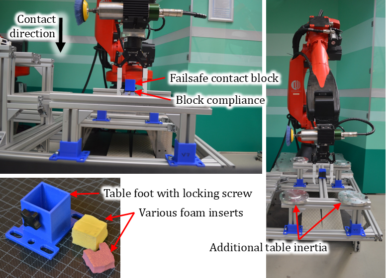
A compliant table, seen in Figure 9, was used to investigate the impact of location and quantity of compliance on the ability to detect contact. By varying the compliance in the feet and contact surface, as well as the inertia of the table, a range of contact responses were achieved as seen in Figure 10. A simple contact detection threshold of $6$ N was applied, and the performance can be seen in the attached video. Model identification was done as above, but a two-inertia model was found to provide better model fit, requiring a straightforward extension to (18) which is omitted due to space constraints but in the published code.

The information gain, calculated with (20) at the state $t=0.002$ after contact, is compared with the time taken to detect the contact in Figure 11. It can be seen that as information gain increases, time to detect contact decreases.

The configurations where contact compliance was removed, and where additional weight was added to the table, had higher information gain and a higher contact velocity could be safely achieved - further detailed plots are available online with the experimental data.

References

- [1] G. Bledt, P. M. Wensing, S. Ingersoll, and S. Kim, “Contact Model Fusion for Event-Based Locomotion in Unstructured Terrains,” in 2018 IEEE International Conference on Robotics and Automation (ICRA), May 2018, pp. 4399–4406.
- [2] M. Vecerik, O. Sushkov, D. Barker, T. Rothörl, T. Hester, and J. Scholz, “A Practical Approach to Insertion with Variable Socket Position Using Deep Reinforcement Learning,” arXiv:1810.01531 [cs], Oct. 2018.
- [3] D. E. Stewart, “Rigid-Body Dynamics with Friction and Impact,” SIAM Review, vol. 42, no. 1, pp. 3–39, Jan. 2000.
- [4] A. M. Castro, A. Qu, N. Kuppuswamy, A. Alspach, and M. Sherman, “A Transition-Aware Method for the Simulation of Compliant Contact With Regularized Friction,” IEEE Robotics and Automation Letters, vol. 5, no. 2, pp. 1859–1866, Apr. 2020.
- [5] M. V. Minniti, R. Grandia, K. Fäh, F. Farshidian, and M. Hutter, “Model predictive robot-environment interaction control for mobile manipulation tasks,” in 2021 IEEE International Conference on Robotics and Automation (ICRA). IEEE, 2021, pp. 1651–1657.
- [6] M. Posa, C. Cantu, and R. Tedrake, “A direct method for trajectory optimization of rigid bodies through contact,” The International Journal of Robotics Research, vol. 33, no. 1, pp. 69–81, 2014.
- [7] Feng Pan and J. M. Schimmels, “Robust procedures for obtaining assembly contact state extremal configurations,” in IEEE International Conference on Robotics and Automation, 2004. Proceedings. ICRA ’04. 2004, vol. 1, Apr. 2004, pp. 972–977 Vol.1.
- [8] J. De Schutter, T. De Laet, J. Rutgeerts, W. Decré, R. Smits, E. Aertbeliën, K. Claes, and H. Bruyninckx, “Constraint-based task specification and estimation for sensor-based robot systems in the presence of geometric uncertainty,” The International Journal of Robotics Research, vol. 26, no. 5, pp. 433–455, 2007.
- [9] M. P. Polverini, A. M. Zanchettin, and P. Rocco, “A constraint-based programming approach for robotic assembly skills implementation,” Robotics and Computer-Integrated Manufacturing, vol. 59, pp. 69–81, 2019.
- [10] W. Meeussen, J. Rutgeerts, K. Gadeyne, H. Bruyninckx, and J. De Schutter, “Contact-state segmentation using particle filters for programming by human demonstration in compliant-motion tasks,” IEEE Transactions on Robotics, vol. 23, no. 2, pp. 218–231, 2007.
- [11] S. Pfrommer, M. Halm, and M. Posa, “ContactNets: Learning of Discontinuous Contact Dynamics with Smooth, Implicit Representations,” arXiv preprint arXiv:2009.11193, 2020.
- [12] J. Rosell, L. Basanez, and R. Suárez, “Contact Identification for robotic assembly tasks with uncertainty,” IFAC Proceedings Volumes, vol. 33, no. 27, pp. 141–146, 2000.
- [13] L. Roveda, “Sensorless environment stiffness and interaction force estimation for impedance control tuning in robotized interaction tasks,” Autonomous Robots, p. 18.
- [14] I. F. Jasim and P. W. Plapper, “Contact-state recognition of compliant motion robots using expectation maximization-based Gaussian mixtures,” in ISR/Robotik 2014; 41st International Symposium on Robotics; Proceedings Of. VDE, 2014, pp. 1–8.
- [15] T. Ren, Y. Dong, D. Wu, and K. Chen, “Collision detection and identification for robot manipulators based on extended state observer,” Control Engineering Practice, vol. 79, pp. 144–153, 2018.
- [16] K. Haninger and D. Surdilovic, “Multimodal Environment Dynamics for Interactive Robots: Towards Fault Detection and Task Representation,” in Proc. IEEE/RSJ Intl Conf on Intelligent Robots and Systems (IROS), 2018, pp. 6932–6937.
- [17] S. Golz, C. Osendorfer, and S. Haddadin, “Using tactile sensation for learning contact knowledge: Discriminate collision from physical interaction,” in 2015 IEEE International Conference on Robotics and Automation (ICRA). IEEE, 2015, pp. 3788–3794.
- [18] P. M. Wensing, A. Wang, S. Seok, D. Otten, J. Lang, and S. Kim, “Proprioceptive Actuator Design in the MIT Cheetah: Impact Mitigation and High-Bandwidth Physical Interaction for Dynamic Legged Robots,” IEEE Transactions on Robotics, vol. 33, no. 3, pp. 509–522, Jun. 2017.
- [19] A. Bicchi and G. Tonietti, “Fast and ”Soft-Arm” Tactics,” IEEE Robotics & Automation Magazine, vol. 11, no. 2, pp. 22–33, Jun. 2004.
- [20] K. Haninger and D. Surdilovic, “Bounded Collision Force by the Sobolev Norm: Compliance and Control for Interactive Robots,” in 2019 IEEE International Conference on Robotics and Automation (ICRA), 2019, pp. 8259–8535.
- [21] S. D. Eppinger and W. P. Seering, “Three dynamic problems in robot force control,” IEEE Transactions on Robotics and Automation, vol. 8, no. 6, pp. 751–758, 1992.
- [22] G. Pratt and M. Williamson, “Series elastic actuators,” in 1995 IEEE/RSJ International Conference on Intelligent Robots and Systems 95. ’Human Robot Interaction and Cooperative Robots’, Proceedings, vol. 1, Aug. 1995, pp. 399–406 vol.1.
- [23] E. A. Bolıvar-Nieto, G. C. Thomas, E. Rouse, and R. D. Gregg, “Convex Optimization for Spring Design in Series Elastic Actuators: From Theory to Practice,” 2021.
- [24] S. Haddadin, K. Krieger, A. Albu-Schäffer, and T. Lilge, “Exploiting elastic energy storage for “blind” cyclic manipulation: Modeling, stability analysis, control, and experiments for dribbling,” IEEE Transactions on Robotics, vol. 34, no. 1, pp. 91–112, 2018.
- [25] K. Haninger, “Minimum directed information: A design principle for compliant robots,” in IEEE International Conference on Robotics and Automation (ICRA), 2021.
- [26] M. Hamaya, R. Lee, K. Tanaka, F. von Drigalski, C. Nakashima, Y. Shibata, and Y. Ijiri, “Learning robotic assembly tasks with lower dimensional systems by leveraging physical softness and environmental constraints,” in 2020 IEEE International Conference on Robotics and Automation (ICRA). IEEE, 2020, pp. 7747–7753.
- [27] P. Tomei, “A simple PD controller for robots with elastic joints,” Automatic Control, IEEE Transactions on, vol. 36, no. 10, pp. 1208–1213, 1991.
- [28] C. Della Santina, M. Bianchi, G. Grioli, F. Angelini, M. Catalano, M. Garabini, and A. Bicchi, “Controlling Soft Robots: Balancing Feedback and Feedforward Elements,” IEEE Robotics Automation Magazine, vol. 24, no. 3, pp. 75–83, Sep. 2017.
- [29] T. J. Debus, P. E. Dupont, and R. D. Howe, “Distinguishability and identifiability testing of contact state models,” Advanced Robotics, vol. 19, no. 5, pp. 545–566, 2005.
- [30] M. W. Spong, “Modeling and control of elastic joint robots,” Journal of dynamic systems, measurement, and control, vol. 109, no. 4, pp. 310–318, 1987.
- [31] N. Kashiri, J. Malzahn, and N. G. Tsagarakis, “On the Sensor Design of Torque Controlled Actuators: A Comparison Study of Strain Gauge and Encoder-Based Principles,” IEEE Robotics and Automation Letters, vol. 2, no. 2, pp. 1186–1194, Apr. 2017.
- [32] S. Thrun, “Probabilistic robotics,” Communications of the ACM, vol. 45, no. 3, pp. 52–57, 2002.
- [33] S. Haddadin, A. De Luca, and A. Albu-Schäffer, “Robot collisions: A survey on detection, isolation, and identification,” IEEE Transactions on Robotics, vol. 33, no. 6, pp. 1292–1312, 2017.
- [34] T. M. Cover, Elements of Information Theory. John Wiley & Sons, 1999.
- [35] A. Kolchinsky and B. D. Tracey, “Estimating mixture entropy with pairwise distances,” Entropy, vol. 19, no. 7, p. 361, 2017.
- [36] M. F. Huber, T. Bailey, H. Durrant-Whyte, and U. D. Hanebeck, “On entropy approximation for Gaussian mixture random vectors,” in 2008 IEEE International Conference on Multisensor Fusion and Integration for Intelligent Systems. IEEE, 2008, pp. 181–188.
- [37] T.-C. Kao and G. Hennequin, “Automatic differentiation of Sylvester, Lyapunov, and algebraic Riccati equations,” arXiv:2011.11430 [cs, math], Nov. 2020.
- [38] K. Haninger, M. Radke, A. Vick, and J. Kruger, “Towards High-Payload Admittance Control for Manual Guidance with Environmental Contact,” IEEE Robotics and Automation Letters, 2022.
- [39] J. A. Andersson, J. Gillis, G. Horn, J. B. Rawlings, and M. Diehl, “CasADi: A software framework for nonlinear optimization and optimal control,” Mathematical Programming Computation, vol. 11, no. 1, pp. 1–36, 2019.