Quantum eraser from duality–entanglement perspective

Introducing the notion of wave-particle duality, Louis de Broglie put forwards one of the most perplexing concepts of quantum physics in 1923 De Broglie 1923. Later, this counterintuitive feature was generalazed as the complementarity principle by Niels Bohr Bohr 1928. To be more specific, according to the complementarity principle a quantum object has physical properties which are equally real but mutually exclusive Bohr 1928. To illustrate, considering an interferometry setting, all information contained in a quantum system is captured by both wave and particle nature of the system; however, measuring one of the properties prohibits the other to be observed Bohr 1928. This setting could be understood by examining a single photon that is subjected to an interferometer. In such a discipline, the particle nature of the light is captured by our knowledge about the photon path Englert et al. 1994; Dürr et al. 1998. In contrast, the wave nature of the light is determined by the visibility of the interference pattern on the screen Englert et al. 1994; Dürr et al. 1998.

The notion of the complementarity principle has been a subject of heated debates since it was first introduced Englert et al. 1994; Przibram et al. 1967; nevertheless, it was not mathematically quantified until 1979, when Wootters and Zurek quantitatively formulated the wave and the particle characteristics of quantum systems Wootters and Zurek 1979. This quantification, was later expressed as an explicit inequality $\mathcal{P}^{2}+\mathcal{V}^{2}\leq 1$ Greenberger and Yasin 1988, where $\mathcal{P}$ stands for the path information (prior path predictability) of a quantum particle, and $\mathcal{V}$ stands for the interference pattern, visibility, addressing the wavelike behavior of the light Glauber 1986; Mandel 1991; Jaeger et al. 1993; Englert 1996; Rab et al. 2017. Since then, there has been a great deal of interest in various aspects of the quantum duality Bera et al. 2015; Qureshi and Siddiqui 2017; Liu et al. 2012; Huang et al. 2013; Basso and Maziero 2020; Englert and Bergou 2000.

Considering the wave-particle duality in Young double-slit experiment, Scully and Drühl realized a profoundly novel feature that enables recovery of the interference pattern via erasing the which-path information Scully and Drühl 1982; a phenomenon that they referred to as ”quantum eraser”. This peculiar effect was later experimented by Kim, et. al. Kim et al. 2000. As a counterintuitive aspect of quantum eraser, one may choose to erase the which-path information even after the photon is registered on the screen, yet restore the interference pattern Aharonov and Zubairy 2005; Kim et al. 2000, shedding new lights on the dramatic departure of quantum world from the classical realm Aharonov and Zubairy 2005; Kim et al. 2000; Zubairy 2020.
More recently, it has been discovered that entanglement plays a significant role in the notion of the wave-particle duality. In fact, it was observed that entanglement controls the duality nature of the quantum systems Jakob and Bergou 2007; de Melo et al. 2007. More specifically, taking quantum entanglement into the consideration, the duality inequality for the double-slit experiment, $\mathcal{P}^{2}+\mathcal{V}^{2}\leq 1$, could be reformulated as the triality relation $\mathcal{P}^{2}+\mathcal{V}^{2}+\mathcal{C}^{2}=1$ Jakob and Bergou 2007; de Melo et al. 2007; Qian et al. 2018. In this equality, $\mathcal{C}$ is the concurrence, as a measure of two-qubit entanglement Wootters 1998. This finding exactly quantifies the relation between the complementarity notion of a quantum system and quantum entanglement. Interestingly, a tight connection between the stereographic geometry and the complementarity-entanglement triality of a quantum system was recently established Maleki 2019, enabling the full geometric proof and the description of the notion of the complementarity-entanglement triality.

In this work, we show that the complementarity-entanglement triality quantified in terms of $\mathcal{P}$, $\mathcal{V}$ and $\mathcal{C}$ captures all the physics of the quantum eraser protocol, in its general setting. In other words, once the concurrence and the quantitative duality relations are taken into account, we can attain the full description of the quantum eraser protocol, providing insights into the fabric of the quantum complementarity, entanglement and quantum eraser, as the basic concepts that bear the key to the fundamental characteristics of the quantum mechanics, and uncovering their relations. As we show below in this work, a partial erasure of the which-path information, and hence, partial recovery of the visibility can exactly be realized and characterized using the triality relation. As one main aspect of our work, we extend our analyses to a broader context where the interactions of the system with the external degrees of freedom (i.e., losses to environment) can also be taken into the consideration, hence, providing a general analysis of the setting.

An elegant experimental realization of the quantum eraser strategy was demonstrated in Kim et al. 2000. The quantum eraser setup that we briefly introduce in this section is investigated by Aharanov and Zubairy in Aharonov and Zubairy 2005 and analyzed in a recent book by Zubairy in Zubairy 2020, which are akin to the setup in Kim et al. 2000. The scheme of the setup, for the quantum eraser protocol, is depicted in Fig. 1 Aharonov and Zubairy 2005; Zubairy 2020. Accordingly, each pinhole in the double-slit experiment is replaced by a four-level atom. The atoms become excited by the single-photon pulses $I_{1}$ and $I_{2}$. The decay of the atoms generates correlated $\gamma$ and $\phi$ photons by either atoms at site 1 or site 2. The energy-level transition diagram and generation of the photon pairs is shown in Fig. 1. In this setting, each register of $\gamma$ photon on the screen is accompanied by a click on the left-hand-side detectors $D_{1}-D_{4}$. Repeating this scattering-detection from the atoms for a large number of times and sorting out the specific registers of the $\gamma$ photon for which a certain detector gets a click, one can recover a destroyed interference pattern by erasing the which-path information. The distribution of the registered $\gamma$ photons on the screen, for the different detection setting of the $\phi$ photons, is depicted in Fig. 2.

To lay out the essence of the quantum eraser in Fig. 1, we start with the state of the photons emitted by the atoms located at sites 1 and 2 as Aharonov and Zubairy 2005; Zubairy 2020

where $\ket{10}_{\gamma}$ stands for the emission of one $\gamma$ photon from site 1 and zero $\gamma$ photon from site 2 (corresponding to the upper path), and similarly $\ket{10}_{\phi}$ stands for the emission of one $\phi$ photon from site 1 and zero $\phi$ photon from site 2 (corresponding to the lower path), etc.

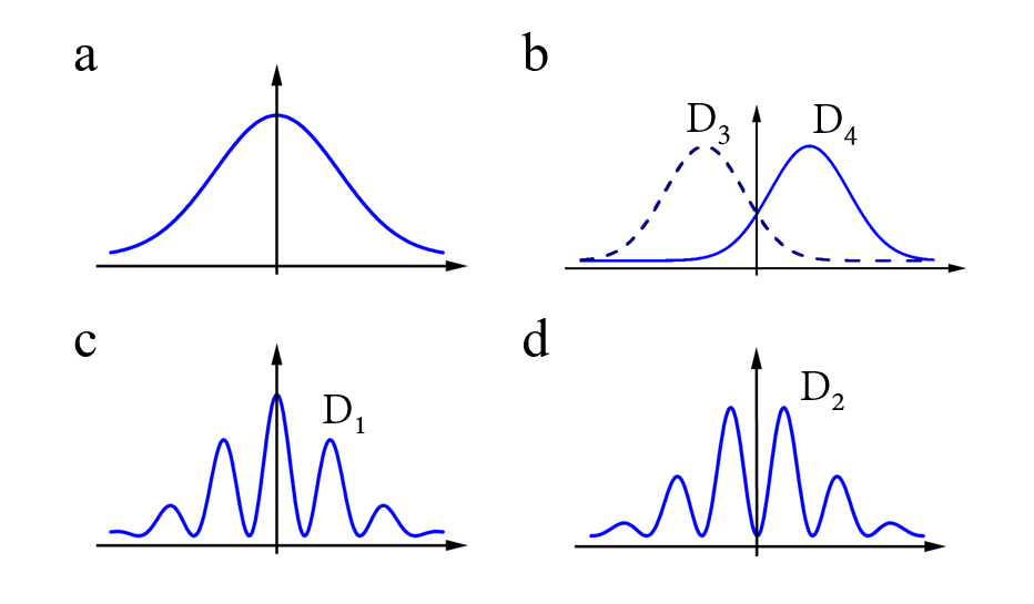
Now, if $B_{1}$ and $B_{2}$ are removed (i.e., if they are completely transmitting beam-splitters (BSs)), a $\phi$ photon will be registered at either $D_{3}$ or $D_{4}$. Considering a click at $D_{3}$, we attain the full which-path information that the photon pair is generated at site 1. Hence, no interference is expected. In this setting, the state $\ket{\Psi}_{0}$ collapses to $\ket{10}_{\gamma}\ket{10}_{\phi}$. A similar consideration is valid for the register of photon in $D_{4}$, where the state $\ket{\Psi}_{0}$ collapses to $\ket{01}_{\gamma}\ket{01}_{\phi}$. In this setting also, as is depicted in Fig. 2(b), there is no interference.

In contrast, when we mount mirrors at $B_{1},B_{2}$ (i.e., if they are perfectly reflecting BSs), there will be a click at either $D_{1}$ or $D_{2}$. The state of the system after passing though the 50:50 beam-splitter $B_{3}$ becomes

When $D_{1}$ clicks the state collapses to $\ket{\gamma_{+}}$, and alternatively, when $D_{2}$ clicks it collapses into $\ket{\gamma_{-}}$, where

We demonstrate in Fig. 2(c,d) the distribution of $\gamma$ photon state $\ket{\gamma_{+}}$ and $\ket{\gamma_{-}}$, where the interference pattern from each detection is attainable. While, if no detection is made on the $\phi$ photons Fig. 2(a) must be attained.

It is worthwhile to mention that an alternative method of attaining which-path information is to setup mirrors at $B_{1}$ and $B_{2}$ and remove $B_{3}$ instead. In this setting, the presence of $B_{3}$ enables the erasure of the which-path information and the recovery of the interference patterns.

Considering the wave-particle duality scenario, we can encode the existence of a single $\gamma$ photon in path 1 as $\ket{\mathbf{0}}:=\ket{10}$, and the existence of a single $\gamma$ photon in path 2 as $\ket{\mathbf{1}}:=\ket{01}$. The single photon subjected to the double-slit could be correlated to some external degrees of freedom, akin to the correlation with the $\phi$ photons in the eraser experiment. The entire system of the photon registered on the screen and the correlated system could be expressed as

$c_{1}$ and $c_{2}$ being the complex coefficients. The wave-particle duality principle could be formulated as $\mathcal{P}^{2}+\mathcal{V}^{2}\leqslant 1$, where $\mathcal{P}$ stands for the path predictability (prior which-path information, that is also referred to as the path distinguishability in some literature Liu et al. 2012; Huang et al. 2013; Qian et al. 2018) of a quantum object which accounts for the particlelike behavior of the photon, and $\mathcal{V}$ represents the interference pattern visibility, addressing the wavelike characteristics of the system Jaeger et al. 1993; Englert 1996.

The wavelike behavior can be quantified via the fringe visibility on the screen as Maleki 2019

where, $p_{D}^{max}$ and $p_{D}^{min}$ are the maximum and minimum probabilities of the photon (photons intensities) registered on the screen, respectively. Alternatively, which-path information can be quantified by Maleki 2019

in which $p_{0}$ and $p_{1}$ represent the probabilities of the photon taking the path 1 or path 2, respectively.

The state in Eq. (4) recasts a two-qubit state via a proper encoding of the computational basis Maleki 2019. With this observation, once the entanglement is taken into the consideration we attain Jakob and Bergou 2007; de Melo et al. 2007; Qian et al. 2018; Maleki 2019

Here, $\mathcal{C}$ is the concurrence as a measure of two-qubit entanglement Wootters 1998. The entanglement quantified in the concurrence framework, is defined through the $R$ matrix as $R=\sqrt{\sqrt{\rho}\bar{\rho}\sqrt{\rho}}$, with $\bar{\rho}=(\sigma_{y}\otimes\sigma_{y})\rho^{*}(\sigma_{y}\otimes\sigma_{y})$. Sorting out the eigenvalues of the matrix $R$ in nonincreasing order, one can determine the concurrence as $\mathcal{C}=\text{max}\{0,\lambda_{0}-\lambda_{1}-\lambda_{2}-\lambda_{3}\}$ Wootters 1998, where $\lambda_{i}$s are the eigenvalues of the matrix $R$ in the deceasing order.

The concurrence of a pure two-qubit state could be determined in terms of the purity of one of the subsystems as $\mathcal{C}^{2}=2[1-\text{Tr}(\rho^{2})]$ Maleki 2019; Wootters 2001, from which we find

Now, we consider a rather general setting for the quantum eraser protocol and lay out its connection to duality–entanglement relation $\mathcal{P}^{2}+\mathcal{V}^{2}+\mathcal{C}^{2}=1$. As we demonstrate below in this work, the physical picture of the quantum eraser experiment could be fully analyzed via duality–entanglement relation. To this aim, we consider the quantum eraser setup that was discussed earlier. However, to lay out a more general setting, we assume that the probability of the generating photon pairs in site 1 and site 2 are not necessarily symmetric, such that $|c_{1}|^{2}$ and $|c_{2}|^{2}$ represent the probability of the pair generation in site 1 and site 2, respectively. The state of the entire system could then be written as

This state simply reduces to Eq. (1) if $c_{1}=c_{2}$. Using this state, we immediately find the reduced density matrix of the $\gamma$ photon by tracing over the $\phi$ photon, from which, we find $\mathcal{P}=\left||c_{1}|^{2}-|c_{2}|^{2}\right|$, $\mathcal{V}=0$, and $\mathcal{C}=2|c_{1}c_{2}|$. Therefore, generation of $\phi$ photon is enough for the vanishing of the fringe visibility. In this case we have $\mathcal{P}^{2}+\mathcal{C}^{2}=1$, as expected. However, detecting $\phi$ photon via $D_{1(2)}$, reduces the $\gamma$ photon state to $\ket{\Psi}=c_{1}\ket{10}_{\gamma}\pm c_{2}\ket{01}_{\gamma}$. In this setting, the entanglement vanishes ($\mathcal{C}=0$), and we find $\mathcal{P}=\left||c_{1}|^{2}-|c_{2}|^{2}\right|$, $\mathcal{V}=2|c_{1}c_{2}|$, leading to $\mathcal{P}^{2}+\mathcal{V}^{2}=1$.

The state in Eq. (1), as well as Eq. (9) are pure states, where no interaction with any other degrees of freedom or losses to environment is taken into consideration. Considering such interactions, the entire state of $\gamma$ and $\phi$ photons will be a mixed state. In a realistic setting the states do not remain pure as the losses into environment are usually unavoidable Kim et al. 2000. To address this kind of more realistic settings, we need to take further degrees of freedom into the account. As an interesting route to incorporate such external degrees of freedom, and more specifically to simulate the effects of decoherence, polarizers could be employed, similar to the approaches taken in Kim et al. 2012; Kim et al. 2009 for simulation of decoherence Escher et al. 2011. With this strategy in mind, we mount the polarizers $S_{1}$ and $S_{2}$ for the photons $\phi_{1}$ and $\phi_{2}$, respectively [see Fig. 3]. Considering $\ket{S_{1}}$ and $\ket{S_{2}}$ as the polarization states of the site 1 and site 2, the overlap of the polarizations of the $\phi$ photons can be given by $q=\bra{S_{1}}{S_{2}}\rangle$, with $0\leqslant|q|\leqslant 1$. Note that when $\ket{S_{1}}$ and $\ket{S_{2}}$ are the same, the polarization degree of freedom has no effect on the quantum eraser setup. The state of the entire system after the $\phi$ photon passes through the polarizer can be written as

The density operator in the $\gamma$ and the $\phi$ photons subspace can be attained via $\rho=\text{Tr}_{S}(\ket{\Psi}_{0}\bra{\Psi}_{0})$, such that

Note that this density matrix recovers the pure state Eq. (9) for $q=1$, while it represents a mixed state for $q\neq 1$, and the entire coherence term vanishes when $q=0$.

Again, in order to lay out a more general setting we assign arbitrary reflectivity and transmitivity to each BS such that the each $B_{i}$ is characterized by the reflection factor $r_{i}$ and the transmition factor $t_{i}$, satisfying $|r_{i}|^{2}+|t_{i}|^{2}=1$. We can recover the original scheme of the quantum eraser, by setting $|t_{1}|=|t_{2}|=1$ for the scenario where $D_{3}$ and $D_{4}$ click. In the opposite, we can set $|r_{1}|=|r_{2}|=1$ for the scenario where $D_{1}$ and $D_{2}$ click.

With this description, after passing through $B_{1}$ and $B_{2}$, the state of the system degenerates into

where $\ket{1000}_{\phi}$ represents the setting that one $\phi$ photon is on path $a$, and no $\phi$ photon exist on paths $b,c$ and $d$, etc.

After passing though $B_{3}$, the entire state of the system can be written as

where $|\psi_{1}\rangle={N_{1}^{-1}}[c_{1}r_{1}r_{3}|10\rangle_{\gamma}|S_{1}\rangle+c_{2}r_{2}t_{3}|01\rangle_{\gamma}\left|S_{2}\right\rangle]$, $|\psi_{2}\rangle={N_{2}^{-1}}[c_{1}r_{1}t_{3}|10\rangle_{\gamma}|S_{1}\rangle-c_{2}r_{2}r_{3}|01\rangle_{\gamma}\left|S_{2}\right\rangle]$, $\left|\psi_{3}\right\rangle=|10\rangle_{\gamma}\left|S_{1}\right\rangle$ and $\left|\psi_{4}\right\rangle=|01\rangle_{\gamma}\left|S_{2}\right\rangle$. Here $N_{i}$ is determined by the normalization of $\ket{\psi_{i}}$, $i=1,2$.

Once this state is given, we can determine the state of the $\gamma$ photon for the different click of the detectors. When $D_{3}$ and $D_{4}$ click, the $\gamma$ photon state collapse to $\ket{\gamma}_{3}=\ket{10}_{\gamma}$ and $\ket{\gamma}_{4}=\ket{01}_{\gamma}$, respectively. While a click on $D_{1}$ reduces the state of the $\gamma$ photon to $\rho_{\gamma}^{(1)}$ and a click on $D_{2}$ reduces the state of the $\gamma$ photon to $\rho_{\gamma}^{(2)}$, such that

The probabilities of the click for each detector is given by $p_{1}=N_{1}^{2}=|c_{1}r_{1}r_{3}|^{2}+|c_{2}r_{2}t_{3}|^{2}$, $p_{2}=N_{2}^{2}=|c_{1}r_{1}t_{3}|^{2}+|c_{2}r_{2}r_{3}|^{2}$, $p_{3}=|c_{1}t_{1}|^{2}$ and $p_{4}=|c_{2}t_{2}|^{2}$.

Now, having these relations in hand, we can analyze the different scenarios for the generalized quantum eraser protocol. The click of the detector $D_{1}$ or $D_{2}$ contributes to the fringe visibility and the erasing of the which-path information. Without loss of generality, we analyze the click in $D_{1}$, where the state collapses into $\rho_{\gamma}^{(1)}$. In this case, the visibility, the which-path information and the entanglement are determined as

leading to $\mathcal{P}^{2}_{1}+\mathcal{V}^{2}_{1}+\mathcal{C}^{2}_{1}=1$. It is worth mentioning that for calculating the entanglement in the state $\ket{\Psi}_{1}$, we consider the computational basis of the first subsystem as $|0\rangle\equiv|10\rangle_{\gamma}$ and $|1\rangle\equiv|01\rangle_{\gamma}$, and the computational basis of the second subsystem as $|0\rangle\equiv|S_{1}\rangle$ and $|1\rangle\equiv|S_{2}\rangle$. We also note that a similar setting could be obtained for the click in $D_{2}$. Now, to recover the conventional case of the quantum eraser protocol discussed earlier, we can take $|c_{1}|=|c_{2}|$, $|r_{1}|=|r_{2}|=1$ and $q=1$; and take $B_{3}$ as a 50:50 BS. In this scenario, $\mathcal{P}_{1}$ and $\mathcal{C}_{1}$ shall be zero, and $\mathcal{V}_{1}=1$, with the collapsed state $\ket{\gamma_{+}}$. Alternatively, the detection of the photons in $D_{3}$ and $D_{4}$ always provides $\mathcal{P}_{1(2)}=1$, hence, zero visibility is available. However, considering Eqs. (13)-(15), we have provided a much more general setting where even partial visibility and partial which-path information could also be quantitatively captured in this setting. Each element in Eq. (15) can vary from zero to one, depending on the specific parameter choices. As a specific setting, the condition $\mathcal{P}_{1}=0$, provides $|c_{1}r_{1}r_{3}|=|c_{2}r_{2}t_{3}|$. where no which-path information exists. Therefore, the full erasure of the path information can be achieved via specific control of the parameters. In this scenario $\mathcal{V}_{1}=|q|$ and $\mathcal{C}_{1}=\sqrt{1-|q|^{2}}$. Alternatively, taking $|c_{1}|=|c_{2}|$ and $|r_{1}|=|r_{2}|=1$ yields $\mathcal{P}_{1}=1$ for $t_{3}=1$ and also for $r_{3}=1$. In this setting, if $B_{3}$ is fully reflective, photons reaching $D_{1}$ always come from site 2, and those reaching $D_{2}$ always come from site $1$, making the full path information available. As is readily seen from Eq. (15) the visibility is proportional to $q$. Therefore, the vanishing of the coherence term ($q=0$) destroys the visibility, regardless of which detector clicks. In general, the upper bound to the visibility can be given by $\mathcal{V}\leqslant q$.

In Fig. 4 we provide different quantum eraser scenarios, where the duality–entanglement relation provides the full description of the settings. Accordingly, Fig. 4(a) provides the effect of the variation of the polarization degree of freedom. When the two polarizations are orthogonal zero fringe visibility is available. This is due to the fact that the entanglement becomes maximum with respect to the polarization degree of freedom. In Fig. 4(b), the scenario is depicted when $|c_{1}|$ varies from 0 to 1. In this case, the which-path information can become zero by adjusting the other parameters (when the visibility and the entanglement are maximum), while $|c_{1}|=0,1$ provides the full which-path information as expected. In Fig. 4(c), the reflection factor of the first BS is varied. As is shown, the maximum of the visibility and the entanglement is attained when the reflectivity is 1. This setting agrees with the which-path information erasing, as the complete reflectivity diminishes the which-path information gain via detector $D_{3}$. In this setting, the photon is sent to $D_{1}$ and $D_{2}$, and hence, the which-path information could be partially erased, and partial visibility could be recovered. Fig. 4(d) presents the duality-entanglement elements in terms of the reflection factor of the third BS. As is shown, we can control all the elements by changing the reflectively of the third BS, where a partial recovery of the interference and entanglement could be manipulated.

In the context of the wave-particle duality, one can also introduce the concept of distinguishability Englert 1996. It can be shown that distinguishability is related to predictability and entanglement through $\mathcal{D}_{1}^{2}=\mathcal{P}_{1}^{2}+C_{1}^{2}$ Qureshi 2021. Considering the state

and Eq. (15), we can introduce the distinguishability as

In Eq. (16), we can define the probabilities $p_{1}=|c_{1}r_{1}r_{3}|^{2}/N_{1}^{2}$ and $p_{2}=|c_{2}r_{2}t_{3}|^{2}/N_{1}^{2}$, and rewrite the distinguishability as

Wave-particle duality is a perplexing feature at the heart of quantum mechanics which refers to the mutually exclusive dual attributes of quantum objects as the wave and the particle. Quantum eraser presenting a counterintuitive aspect of the wave-particle duality enables recovery of the interference pattern via erasing the which-path information. In this work, we showed that quantum eraser can be quantitatively analyzed in terms of wave-particle-entanglement triality equality. In other words, we showed that wave-particle-entanglement triality captures the entire physics of the quantum erasure. As a part of our analyses, we found that a controllable partial erasure of the which-path information is attainable, enabling the partial recovery of the quantum interference. The interesting physics behind the quantum eraser comes from quantum entanglement, which enables the indirect which-path information gain through the detection of the entangled photon. On the other hand, the duality-entanglement relation is also deeply connected to the quantum entanglement, demonstrating the controlling role of quantum entanglement on the duality. As a result, quantum entanglement is the key to unify these two settings and lay out a general formalism for quantum complementarity. Our study, illuminating the deep connection between quantum eraser protocols and wave-particle-entanglement triality, may shed new light on fundamental aspects of quantum interferometry Zubairy 2020, quantum coherence, and quantum steering Maleki and Ahansaz 2020.

This research is supported by the project NPRP 13S-0205-200258 of the Qatar National Research Fund (QNRF).

References

- De Broglie (1923) L. De Broglie, Nature 112, 540 (1923).
- Bohr (1928) N. Bohr, “The quantum postulate and the recent development of atomic theory 1,” (1928).
- Englert et al. (1994) B.-G. Englert, M. O. Scully, and H. Walther, Scientific American 271, 86 (1994).
- Dürr et al. (1998) S. Dürr, T. Nonn, and G. Rempe, Nature 395, 33 (1998).
- Przibram et al. (1967) K. Przibram, E. Schrödinger, A. Einstein, H. A. Lorentz, and M. Planck, Letters on wave mechanics (Vision, 1967).
- Wootters and Zurek (1979) W. K. Wootters and W. H. Zurek, Physical Review D 19, 473 (1979).
- Greenberger and Yasin (1988) D. M. Greenberger and A. Yasin, Physics Letters A 128, 391 (1988).
- Glauber (1986) R. J. Glauber, Annals of the New York Academy of Sciences 480, 336 (1986).
- Mandel (1991) L. Mandel, Optics Letters 16, 1882 (1991).
- Jaeger et al. (1993) G. Jaeger, M. A. Horne, and A. Shimony, Physical Review A 48, 1023 (1993).
- Englert (1996) B.-G. Englert, Physical Review Letters 77, 2154 (1996).
- Rab et al. (2017) A. S. Rab, E. Polino, Z.-X. Man, N. B. An, Y.-J. Xia, N. Spagnolo, R. L. Franco, and F. Sciarrino, Nature Communications 8, 1 (2017).
- Bera et al. (2015) M. N. Bera, T. Qureshi, M. A. Siddiqui, and A. K. Pati, Physical Review A 92, 012118 (2015).
- Qureshi and Siddiqui (2017) T. Qureshi and M. A. Siddiqui, Annals of Physics 385, 598 (2017).
- Liu et al. (2012) H.-Y. Liu, J.-H. Huang, J.-R. Gao, M. S. Zubairy, and S.-Y. Zhu, Physical Review A 85, 022106 (2012).
- Huang et al. (2013) J.-H. Huang, S. Wölk, S.-Y. Zhu, and M. S. Zubairy, Physical Review A 87, 022107 (2013).
- Basso and Maziero (2020) M. L. Basso and J. Maziero, Journal of Physics A: Mathematical and Theoretical 53, 465301 (2020).
- Englert and Bergou (2000) B.-G. Englert and J. A. Bergou, Optics Communications 179, 337 (2000).
- Scully and Drühl (1982) M. O. Scully and K. Drühl, Physical Review A 25, 2208 (1982).
- Kim et al. (2000) Y.-H. Kim, R. Yu, S. P. Kulik, Y. Shih, and M. O. Scully, Physical Review Letters 84, 1 (2000).
- Aharonov and Zubairy (2005) Y. Aharonov and M. S. Zubairy, Science 307, 875 (2005).
- Zubairy (2020) M. S. Zubairy, Quantum Mechanics for Beginners: With Applications to Quantum Communication and Quantum Computing (Oxford University Press, 2020).
- Jakob and Bergou (2007) M. Jakob and J. A. Bergou, Physical Review A 76, 052107 (2007).
- de Melo et al. (2007) F. de Melo, S. Walborn, J. A. Bergou, and L. Davidovich, Physical Review Letters 98, 250501 (2007).
- Qian et al. (2018) X.-F. Qian, A. Vamivakas, and J. Eberly, Optica 5, 942 (2018).
- Wootters (1998) W. K. Wootters, Physical Review Letters 80, 2245 (1998).
- Maleki (2019) Y. Maleki, Optics Letters 44, 5513 (2019).
- Wootters (2001) W. K. Wootters, Quantum Inf. Comput. 1, 27 (2001).
- Kim et al. (2012) Y.-S. Kim, J.-C. Lee, O. Kwon, and Y.-H. Kim, Nature Physics 8, 117 (2012).
- Kim et al. (2009) Y.-S. Kim, Y.-W. Cho, Y.-S. Ra, and Y.-H. Kim, Optics express 17, 11978 (2009).
- Escher et al. (2011) B. Escher, R. de Matos Filho, and L. Davidovich, Nature Physics 7, 406 (2011).
- Qureshi (2021) T. Qureshi, Optics Letters 46, 492 (2021).
- Maleki and Ahansaz (2020) Y. Maleki and B. Ahansaz, Physical Review A 102, 020402 (2020).