A methodology for detection and localization of fruits
in apples orchards from aerial images
Abstract
Computer vision methods based on convolutional neural networks (CNNs) have presented promising results on image-based fruit detection at ground-level for different crops. However, the integration of the detections found in different images, allowing accurate fruit counting and yield prediction, have received less attention. This work presents a methodology for automated fruit counting employing aerial-images. It includes algorithms based on multiple view geometry to perform fruits tracking, not just avoiding double counting but also locating the fruits in the 3-D space. Preliminary assessments show correlations above 0.8 between fruit counting and true yield for apples. The annotated dataset employed on CNN training is publicly available.
1 Introduction
Crop monitoring is essential for anomaly detection, yield prediction and risk assessment in agriculture, basing the farmer’s interventions. A continuous data collection during the fruits’ growth cycle would allow an accurate modeling of its development, identifying anomalies and bottlenecks. Recently, convolutional neural networks [LeCun et al. 2015] have been employed for ground-level, image-based detection for different fruits [Sa et al. 2016], as apples [Häni et al. 2020] and mangoes [Bargoti and Underwood 2017]. However, just a few works [Liu et al. 2019, Häni et al. 2020, Santos et al. 2020] have addressed the data association problem in fruit counting: how to properly integrate the detections found in multiple images for accurate, row-level fruit tracking.
The present work describes a methodology for detecting and locating apples in orchards from aerial images sequences. This methodology allows not only the detection of fruits in the images, but also their association between images, identifying apples already observed previously, an essential requirement for fruit counting. The identified apples are properly mapped in the three-dimensional space, enabling the analysis of the variability in the field. The present methodology was able to produce promising results from aerial images of about 1 cm per pixel, thus being an alternative for autonomous monitoring of entire plots in orchards by unmanned aerial vehicles (UAVs).
2 Materials and methods
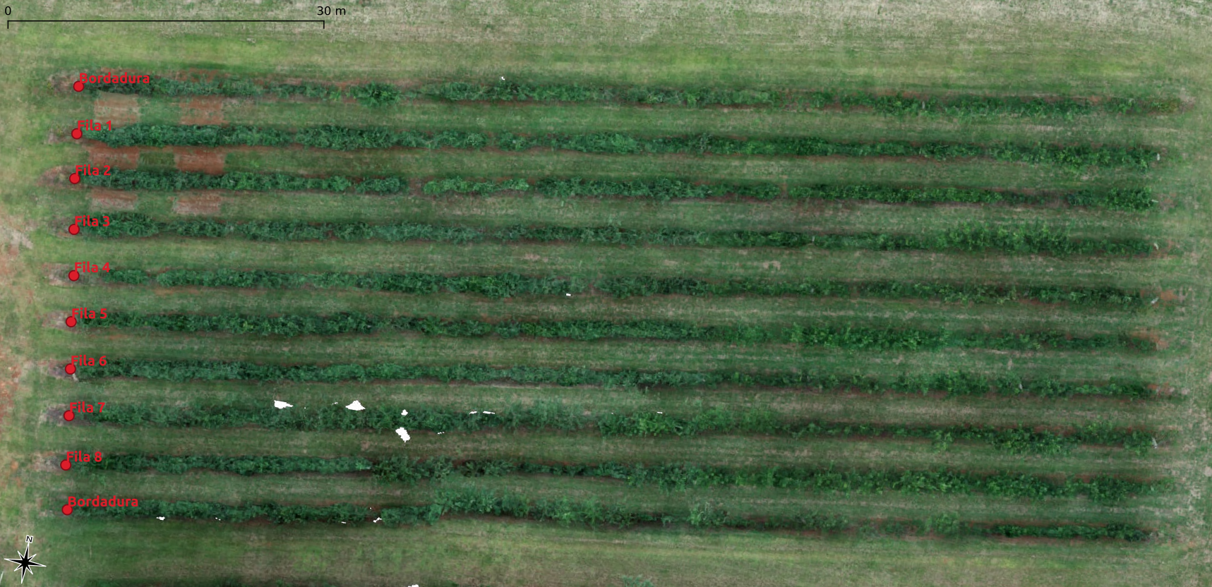
The data employed in the development of the methodology came from a plot located at the Embrapa’s Temperate Climate Fruit Growing Experimental Station at Vacaria-RS (28°30’58.2”S, 50°52’52.2”W). The plot, seen in Figure 1 (a), is composed of 10 rows of apple trees, of which the 8 inner rows contain the plants of interest (the first and last rows are border ones). The rows contain plants of the varieties Fuji (west facing) and Gala (east facing). The images were taken during December 13, 2018. For aerial shots, an UAV (DJI Phantom 4 Pro) performed a 12 m height flight over the orchard’s rows, capturing imagery data in the form of a 4K resolution video ( pixels). The camera tilt is not nadir, allowing a more extensive view of the canopy if compared to a top/nadir one. The terms frame and image will be employed interchangeably in this text.
2.1 Methodology
The methodology consists of three steps. The first one is apple detection performed on each image, using a deep convolutional neural network [LeCun et al. 2015]. The second step estimates the camera position and orientation at each frame, using the structure-from-motion framework from multiple view computer vision [Hartley and Zisserman 2003, Schönberger and Frahm 2016]. The last step, the main contribution in this work, uses projective geometry and directed graphs to represent multiple alternative associations between fruits observed in different frames. Each path in the graph represents an association hypothesis, determining the location of the same fruit in different images, and a greedy algorithm is used to choose the paths.
2.1.1 Apple detection
To this task, we have built an annotated dataset, formed by random selected pixels samples from the frames extracted from the UAV video sequences. The dataset was split in training and test subsets for supervised machine learning, as shown in Table 1. This dataset is publicly available11 1 Available at https://doi.org/10.5281/zenodo.5586329..
| Number of images | Number annotated apples | |
|---|---|---|
| Training | 1025 | 2204 |
| Test | 114 | 267 |
For apple detection, we have employed a Faster R-CNN network [Ren et al. 2017], using a ResNet-50 backbone [He et al. 2016]. We employed the implementation available in PyTorch [Paszke et al. 2019] (see the torchvision library). The details of the training process, including data augmentations techniques, optimizer, batch sizes, number of epochs and hyperparameters can be seen in the publicly available code22 2 Available at https://github.com/thsant/add256-fastercnn. and, due to text size restrictions, they will not be described here.
2.1.2 Relative camera pose estimation
To estimate the camera position at the time of capture for each video frame, we have employed the Structure-from-Motion (SfM) system COLMAP [Schönberger and Frahm 2016]. A SfM system estimates the projection matrix , a matrix, for each image : for each three-dimensional point in the field, its 2-D projection on the image plane of frame can be computed33 3 Points and are in homogenous coordinates, what explains the 1 in their last dimension. by the product
| (1) |
The matrices also allow the computation of the relative position between cameras in the 3-D space by the property . Figure 1 (b) illustrates the position of the UAV camera at the time of each frame capture in the flight over the plot.
 |
 |
| (a) | (b) |
2.1.3 Data association: tracking apples in the frames sequence
Projections matrices and allow the computation of the fundamental matrix [Hartley and Zisserman 2003]. Suppose that a point in the 3-D space is mapped to the 2-D points and on the -th and the -th frames of the video sequence, respectively. The fundamental matrix maps on frame to a epipolar line on frame that contains . In our apple tracking problem, we have , the centroid of the -th apple detected by the neural network on frame . We can employ the fundamental matrix linking frames and to aid us in choosing the most suitable detections to correspond to , as seen in Figure 2.
Consider the centroids of the apples detected by the neural network on the -th frame, . The detection corresponding to apple should be close44 4 Ideally, in a noisy-free, perfect detection scenario, , i.e., . to the line in frame , given by
| (2) |
The fundamental matrix can be computed from the projection matrices by
| (3) |
where is the pseudo-inverse of , and is the epipole, with , i.e., is projection center for the camera in frame [Hartley and Zisserman 2003].

Our proposed apple tracking algorithm employs a graph, , to represent multiple fruit associations hypothesis. Each node corresponds to the centroid of the -th apple detected on a frame . We add an edge iif
| (4) |
being . In other words, we are testing if the distance between the point and the epipolar line is below a threshold . This procedure is performed by the lines 4–9 in Algorithm 1, FruitAssociation. So, an edge in represents a possible association between two detections in different frames. As seen in line 5, for each frame , the following frames are evaluated for associations, what provides robustness to momentaneous misdetections of a fruit by the neural network.
A sequence of edges is a path. Each path represents a possible association hypothesis for a fruit detected in frame and the fruits detected in the following frames. Lines 10-16 in Algorithm 1 implement a path selection process, employing a second algorithm, FruitEstimation3D (Algorithm 2).
Algorithm 2 starts performing a depth-first search (DFS) from node , getting all possible paths starting at . An algorithm based on random sample consensus (RANSAC) [Fischler and Bolles 1981] is employed to estimate the tridimensional point corresponding to a path (an apple’s 3-D position in space). At each iteration, the TriangulationRANSAC algorithm pick three 2-D points, , and (corresponding to nodes , and in a path ) and estimates the 3-D point . The estimation of X is performed by a least-squares minimization algorithm [Hartley and Sturm 1997]. Next, is projected on each frame in the path, defining the points and their corresponding geometrical errors, i.e., the Euclidean distance between and . Nodes in the path whose geometrical error is below the threshold are considered inliers. At each iteration, the RANSAC procedure keeps the point that delivered the largest number of inliers. Algorithm 2 looks for the path presenting the largest rate of inliers , keeping the longest path presenting the largest inlier rate. In other words, the inlier ratio acts as a quality measure for the inter-frame association hypothesis regarding fruit , represented by a path starting from . Once a path is selected, the algorithm remove its edges from (line 16 in Algorithm 1), avoiding those associations to be employed again. However, the nodes are preserved in the graph, allowing fruits occlusions to be considered: fruits that occlude each other can create crossing paths in , i.e., paths sharing nodes.
3 Results and discussion
Figure 3 displays the tracks determined by Algorithm 2 for two different apples. Each line in the figure corresponds to an apple’s track (only the inliers). Note how the look of the fruit and its surroundings varies slightly as the pose (the UAV position) changes from frame to frame. Each track determines the three-dimensional position of an apple: all inliers are used in the final estimation of the fruit’s position in the 3-D space, again by employing the least-squares algorithm [Hartley and Sturm 1997]. Figure 4 displays a total of 9,237 apples found in the plot. Fruits were automatically divided into the ten rows of the field by -means clustering.
Disregarding two rows out of the UAV’s field of view, caused by imprecision in the vehicle positioning system55 5 Precise flights, able to keep the plants in the UAV’s field of view, can be performed by vehicles presenting a precise position control, as a Real-Time Kinematic (RTK) Global Navigation Satellite System (GNSS). Unfortunately, the vehicle used in this work presented an ordinary GNSS system, without the positioning corrections provided by RTK., the observed linear correlation between the counted apples in each row and the row’s yield was 0.11 for Fuji and 0.80 for Gala, considering six rows. However, one of the rows (row 8) looks like a severe outlier: considering just the other five rows, linear correlation is 0.93 for Fuji and 0.88 for Gala. Although promising, the results should be viewed with caution, given that few rows were evaluated, at a single plot. More extensive experiments are yet necessary for a full characterization of uncertainty in yield prediction and the proportion of the fruits that is visible in imagery. It should also be noted that the images were captured in December and the harvest was carried out in February of the following year, which indicates that the methodology has the potential to provide yield estimated in early stages. Indeed, the presented methodology can be employed as a component of a more sophisticated yield prediction system.


4 Conclusions
Fruit detection and tracking can be, in short term, applied to yield prediction and crop monitoring. In the long term, precise detection and 3-D localization can be employed on harvesting by autonomous agents. Detection and tracking allow autonomous agents to estimate their position relative to the fruit, so that accurate handling planning can be performed by the machine. The three-dimensional localization can also characterize the spatial variability of the fruits in the plots, helping on growing management according to precision agriculture practices.
The presented methodology is not restricted to aerial images: the same algorithms could be adapted to images obtained by ground vehicles with embedded cameras. Autonomous aerial vehicles with precise positioning control, such as devices equipped with RTK GNSS, could be used as a row-scanning system able to perform automated field monitoring. New experiments, with a greater variability of plants, management regimes and plant architectures, should be carried out to validate and adapt the methodology for operation in different scenarios, and provide a better characterization of the estimation errors in yield prediction.
Acknowledgments
This work was supported by Brazilian Agricultural Research Corporation (Embrapa) under grant 01.14.09.001.05.04 and by FAPESP under grant (2017/19282-7).
References
- [Bargoti and Underwood 2017] Bargoti, S. and Underwood, J. (2017). Deep fruit detection in orchards. In 2017 IEEE International Conference on Robotics and Automation (ICRA), pages 3626–3633. IEEE.
- [Fischler and Bolles 1981] Fischler, M. A. and Bolles, R. C. (1981). Random sample consensus: a paradigm for model fitting with applications to image analysis and automated cartography. Communications of the ACM, 24(6):381–395.
- [Hartley and Zisserman 2003] Hartley, R. and Zisserman, A. (2003). Multiple View Geometry in Computer Vision. Cambridge University Press, New York, NY, USA, 2 edition.
- [Hartley and Sturm 1997] Hartley, R. I. and Sturm, P. (1997). Triangulation. Computer vision and image understanding, 68(2):146–157.
- [He et al. 2016] He, K., Zhang, X., Ren, S., and Sun, J. (2016). Deep residual learning for image recognition. In Proceedings of the IEEE conference on computer vision and pattern recognition, pages 770–778.
- [Häni et al. 2020] Häni, N., Roy, P., and Isler, V. (2020). A comparative study of fruit detection and counting methods for yield mapping in apple orchards. Journal of Field Robotics, 37(2):263–282.
- [LeCun et al. 2015] LeCun, Y., Bengio, Y., and Hinton, G. (2015). Deep learning. Nature, 521(7553):436–444.
- [Liu et al. 2019] Liu, X., Chen, S. W., Liu, C., Shivakumar, S. S., Das, J., Taylor, C. J., Underwood, J., and Kumar, V. (2019). Monocular Camera Based Fruit Counting and Mapping With Semantic Data Association. IEEE Robotics and Automation Letters, 4(3):2296–2303.
- [Paszke et al. 2019] Paszke, A., Gross, S., Massa, F., Lerer, A., Bradbury, J., Chanan, G., Killeen, T., Lin, Z., Gimelshein, N., Antiga, L., et al. (2019). PyTorch: An imperative style, high-performance deep learning library. In Advances in neural information processing systems, pages 8026–8037.
- [Ren et al. 2017] Ren, S., He, K., Girshick, R., and Sun, J. (2017). Faster r-cnn: Towards real-time object detection with region proposal networks. IEEE Transactions on Pattern Analysis and Machine Intelligence, 39(6):1137–1149.
- [Sa et al. 2016] Sa, I., Ge, Z., Dayoub, F., Upcroft, B., Perez, T., and McCool, C. (2016). Deepfruits: A fruit detection system using deep neural networks. Sensors, 16(8).
- [Santos et al. 2020] Santos, T. T., de Souza, L. L., dos Santos, A. A., and Avila, S. (2020). Grape detection, segmentation, and tracking using deep neural networks and three-dimensional association. Computers and Electronics in Agriculture, 170:105247.
- [Schönberger and Frahm 2016] Schönberger, J. L. and Frahm, J.-M. (2016). Structure-from-motion revisited. In Conference on Computer Vision and Pattern Recognition (CVPR).