ConformalLayers: A non-linear sequential neural network with associative layers
Abstract
Convolutional Neural Networks (CNNs) have been widely applied. But as the CNNs grow, the number of arithmetic operations and memory footprint also increase. Furthermore, typical non-linear activation functions do not allow associativity of the operations encoded by consecutive layers, preventing the simplification of intermediate steps by combining them. We present a new activation function that allows associativity between sequential layers of CNNs. Even though our activation function is non-linear, it can be represented by a sequence of linear operations in the conformal model for Euclidean geometry. In this domain, operations like, but not limited to, convolution, average pooling, and dropout remain linear. We take advantage of associativity to combine all the “conformal layers” and make the cost of inference constant regardless of the depth of the network.
I Introduction
Convolutional Neural Networks (CNNs) are a type of neural network that have become popular in many areas with remarkable accuracy, including Computer Vision. As the network gets, however, higher is the number of operations to perform, and more memory is required for both training and inference.
To make inference, a cheaper operation has become an active topic of research. The primary strategies for accomplishing this are compressing the networks [1, 2, 3, 4, 5, 6], or exploring data organization to fit hardware specificities [7, 8, 9, 10]. But the former strategy leads to modifications to the original architecture. The latter depends on the hardware.
An interesting strategy for simplifying sequential layers of the CNNs would be the combination of adjacent layers by associativity. This idea would not change the network’s architecture and, in the limit, all layers would be combined into a single operator to be applied to the input data. In this paper, the term associativity refer to the mathematical property of a binary operation on a set to satisfy the associative law:
| (1) |
The idea of exploring operations’ associativity to reduce computational costs has been widely explored in other areas, like computer graphics, for example. Unfortunately, composing layers considering existing artificial neural networks is only applicable to sequences of associative operations like convolutions and averages, since typical activation functions turn the layers of sequential networks non-associative.
This work presents a non-linear and differentiable activation function called ReSPro, which stands for Spherical Reflection, Scaling, and Projection. By representing the input data and any map of features produced by the network as points encoded as vectors in the conformal model for Euclidean geometry, ReSPro turns into a sequence of linear transformations in the conformal domain. By adding only one more coefficient to the input data, some linear transformations behave like non-linear, and become suitable as activation function in CNNs. ReSPro and typical operations like convolution, average pooling, dropout, flattening, padding, dilation, and stride can be encoded as rank-2 or rank-3 tensors whose product satisfies the associative law (1). We call ConformalLayers the conformal embedding of sequential layers of CNNs comprised of those operations. By associativity, one sparse matrix and one sparse rank-3 tensor computed after training are enough to encode a sequential CNN made up of any number of conformal layers, making the cost of inference remains constant.
The reduced number of operations required for operating the matrix and the rank-3 tensor resulting from the ConformalLayers with the input data makes our approach well-suited for processing a large number of images, even in devices with limited storage and computational capabilities. To fully explore the advantages of ReSPro and the ConformalLayers, we built a library on top of PyTorch. Such a framework allows the associativity between the sequential layers of CNNs and covers both training and inference processes.
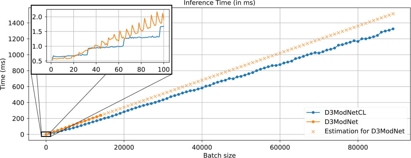
Fig. 1 depicts the differences of inference time of the traditional implementation of a non-associative CNN (D3ModNet) and a similar network implemented using ConformalLayers (D3ModNetCL). The non-associative approach is limited to process 14K images simultaneously on an NVIDIA GTX 1050 Ti (orange line with circles). The ConformalLayers, on the other hand, was able to process 89K images simultaneously on the same hardware (blue line with circles). The orange crosses beyond the limitations of D3ModNet extrapolates its memory and execution times capabilities just for comparison.
Our main contributions can be summarized as:
- •
A new non-linear and differentiable activation function;
- •
The first approach for sequential layers of CNNs where the linear and non-linear layers are associative;
- •
The analysis of the accuracy of conventional CNNs against similar CNNs with ConformalLayers; and
- •
The analysis of the computational performance of conventional CNNs against similar CNNs with ConformalLayers considering the number of layers and batch size.
II Related Work
We group the related works into activation functions, neural network compression, and computationally-efficient CNNs.
Activation Functions
vanishing gradient problem. The sigmoid and hyperbolic tangent are S-shaped activation functions [11]. While the sigmoid may lead to time convergence issues, the hyperbolic tangent mitigates this problem. ReLU [12] provides three main advantages over the hyperbolic tangent: eliminate the problem of vanishing gradient (common in S-shaped functions), add some sparsity to the data, and is computationally simple, although it can map many inputs to zero, preventing the network from learning. GeLU [13] is a non-monotonic non-linear activation function that weights the input by the standard Gaussian cumulative distribution function. Although it is slightly costly, it can provide similar or better results than ReLU. Swish [14] is another non-monotonic activation function that outperforms ReLU-like functions, but with higher computational cost.
To the best of our knowledge, all non-linear activation functions described in the literature are non-associative with linear operations typically used in CNNs. Therefore, they prevent the combination of sequential layers through associativity.
Neural Network Compression
Denton et al. [1] post-process the trained neural networks to iteratively compress each layer and then fixing the accuracy, which presented a speedup at the cost of of accuracy.
Hubara et al. [2] presented a network model using binarization, allowing binary operations instead of products during the inference by the cost of a small percent of accuracy [3].
The lottery ticket hypothesis was postulated by Frankle and Carbin [4]. They state that training a neural network with random weights will most likely provide good results. Still, probably there is a sub-network that is trainable with lower cost and fewer parameters, while providing similar results. Zhou et al. [5] used masking criteria to assess which weights should be pruned in this approach.
By partitioning the set of convolutional filters and using these sets as inputs for an auxiliary neural network, Omidvar et al. [6] generated reusable filters, reducing the number of network parameters. Tetko [15] presented an ensemble of neural networks and -NN which uses the distance between the predicted data and the ground truth to improve the prediction by adjusting the bias on the networks. Both approaches are called “associative” but its important to emphasize that associativity in this paper is related to the property in (1).
The neural network compression techniques discussed here seek to find different networks from those proposed initially or assume less precise data types. We state that it is possible to improve computational performance by combining layers of the network without changing its architecture, as long as an activation function that allows associativity is adopted.
Computationally-Efficient CNNs
YOLO [16] and SqueezeDet [17] are popular real-time CNNs for object detection and classification. While the former is for general purpose, the latter is tailored to autonomous driving.
Alwani et al. [7] leveraged caching aspects in hardware accelerators by observing that each point of a hidden layer depends on a specific region of the input.
MobileNets [8] and EfficientNets [9] are approaches that change the size of a model to fit a resource budget. While the first rely on model depth and image resolution to handle devices with limited capacity, the latter proposes a compound parameter to scale the neural network. In [10], a RNN-based pooling layer is presented to perform data down-sampling as a solution to RAM and energy problems in edge devices.
III ConformalLayers
In this section, we deep dive into the formulation and implementation of the ReSPro function and the ConformalLayers.
III-A ReSPro
Without loss of generality, we consider that the input and output data of the function are finite points in a multidimensional Cartesian space. Each coordinate of these points corresponds to a coefficient of the data. For example, a feature map with pixels and channels is a point with coordinates, which after being transformed by ReSPro maps to . The -to- mapping involves one non-linear and two linear transformations applied to . Fig. 2 illustrates the step-by-step mapping performed by ReSPro. For sake of simplicity, we assume in this example.
Let and be two points lying on the axis (Fig. 2(a)), distant, respectively, and units from the origin, for . In Fig. 2(b), we deliberately added the extra dimension to the Cartesian space and placed the hypersphere (a circle, in this example) with radius and center . In this new space, and . The addition of the dimension to the Cartesian coordinate system is key for defining the non-linear transformation in ReSPro as the spherical reflection of points on . In Fig. 2(b), the spherical reflection maps and to, respectively, and .
Spherical reflection causes points outside the hyperspherical mirror to produce images inside the mirror. The distance of the imaged point to the center of the hypersphere decreases non-linearly as the distance of the original point to the center increases. Notice in Fig. 2(b) that the distance between points and is smaller than the distance between and since is more distant from than . At the limit, points at infinity map to , while points on the hypersphere remain unchanged. By construction, we do not have to care about the reflection of points inside the hyperspherical mirror because is tangent to the space spanned by , and all input points lie in this space (i.e., the coordinate for is zero).
Two linear transformations are applied after spherical reflection. The first is isotropic scaling by a factor of , illustrated in Fig. 2(c), which maps and to and , respectively. The second transformation is the orthogonal projection to the original -dimensional Cartesian space. As can be seen in Fig. 2(d), projects to while projects to . The reasoning for performing scaling followed by projection is to map points that are units away from the origin of the Cartesian space (e.g., ) to points unit away from the origin. The projection also makes the coordinate associated with the extra dimension equal to zero, which can be removed from the resulting point since it is constant.
Formally, ReSPro is a mapping
| (2) |
where are, respectively, the input and output data represented as points, and denotes the -norm of .


Fig. 3 depicts the output of ReSPro for points in with . Notice that the disc shape is due to the region where the function is defined, i.e., .
ReSPro is non-linear, differentiable, invertible, and associative to linear function typically used in CNNs. The verification of the first three properties is straightforward. We demonstrate the last property in Section III-C. In addition, ReSPro is a global activation function. In practical terms, it means that, differently from other activation functions which perform per element transformation, ReSPro activates all the elements simultaneously. This is equivalent to have element-wise activation followed by the normalization to ensure .
III-B Tensor Representation of ReSPro
We use the geometric algebra of the conformal model for Euclidean geometry [18] to perform spherical reflection as orthogonal transformation (hence, a linear transformation) and combine it to isotropic scaling and orthogonal projection. The representational space of the conformal model has two extra dimensions and a degenerate metric [18]. The -dimensional Cartesian space used in Section III-A is embedded in a -dimensional space with basis vectors . The extra dimensions and are geometrically interpretable as the point at the origin and the point at infinity, respectively. In the conformal model, a finite point with coordinates is encoded by the -dimensional vector:
| (3) |
where ⊺ denotes matrix transposition and the scalar does not change the practical interpretation of as the point .
The algebraic manipulation that takes the ReSPro function from its formulation in geometric algebra to tensor algebra is quite involved. Due to space restrictions, it is presented in the Supplementary Material. Here, it is sufficient to show that a -dimensional point encoding input data will be represented by the -dimensional vector:
| (4) |
such that and , for . Vector is mapped to by the ReSPro function as:
| (5) |
such that and , for .
In (4) and (III-B), and are simplified version of (3). They do not include the coefficient related to , since this coefficient is always zero (see Section III-A), nor the coefficient related to , because it can be computed from the other coefficient. The and coefficients are related to the basis vector and act as homogeneous coordinates.
The tensor representation of ReSPro applied to is obtained by rewritten (III-B) as:
| (6) |
where
is a diagonal matrix, and is a rank-3 tensor of size filled with zeros, except for the slice at the bottom, which is the diagonal matrix:
III-C Tensor Representation of ConformalLayers
Recall that in (6) represents a finite point , whose coordinates are the coefficients of some feature map produced by some CNN layer. It is well known that linear function typically used in layers and their configurations can be written in matrix form and applied to vectors by matrix multiplication. For instance, Toeplitz matrices encode -dimensional discrete-time convolutions and can be modified to encode valid cross-correlation [11]; average pooling is the mean filter [19], a particular case of convolution with constant weights; and configurations such as padding, dilation, and stride can be encoded by matrices composed of zeros and ones (see the Supplementary Material). By writing these and other operations in the matrix form, the associativity of the matrix product allows the composition of operations to produce matrices which, when multiplied by a vector , produce the vector representing the output of linear layers. By replacing in (6) by and combining with and , we write:
| (7) |
where is the conformal layer function, a sequence of linear operations applied to , followed by the application of the ReSPro activation function. Here, ⊺ denotes the transposition of the first two dimensions of tensors and matrix transposition.


In CNN architectures, it is typical for linear layers and activation functions to be interspersed. A sequence of conformal layers applied to can be written as:
| (8) |
where . In , the upper index identifies the -th conformal layer, encodes the input data , and encodes the output , whose actual coordinates can be computed as , for .
We expand (8) to model a sequence of conformal layers applied to using tensor form:
| (9) |
where
| (10) |
is a sparse matrix, and
| (11) |
is a tensor of size filled with zeros, except for the slice at the bottom, which is a sparse matrix. The Supplementary Material includes the algebraic manipulation that turns (8) into (9).
Notice that the and components of (9) do not depend on the input data , and they encode a complete sequence of conformal layers. Therefore, after the weights of the CNN be adjusted through the training process, and can be computed once by associativity using (10) and (11), and applied afterward to any to perform inference.
III-D Implementation of ConformalLayers
We have implemented ConformalLayers as an nn.Module of PyTorch 1.811 1 Source code at https://github.com/Prograf-UFF/ConformalLayers/. The cl.ConformalLayers module behaves like an nn.Sequential module, and its current version accepts submodules that mimic the behavior of nn.Conv1d, nn.Conv2d, nn.Conv3d, nn.AvgPool1d, nn.AvgPool2d, nn.AvgPool3d, nn.Dropout, and nn.Flatten, in addition to the cl.ReSPro module. The configuration of existing modules includes stride, zero padding, and dilation whenever necessary.
Fig. 4 shows the algorithm of the forward function implemented by cl.ConformalLayers. During the training process, the cl.ConformalLayers module uses the native PyTorch implementation of supported submodules to compose the network (line 5). The only exception is the cl.ReSPro module, which is implemented according to (III-B), and the computation of the coefficient in all submodules. Once the training process is completed, the cl.ConformalLayers module builds an internal cache containing the sparse matrix (10) and the sparse matrix representing the slice at the bottom of (11). This cache has to be updated only if the user decides to retrain the conformal layers (see lines 4, 9, and 10). As the value of can be different from , the result of applying the sequence of submodules to the input data needs to be divided by to obtain the correct interpretation of the output data (lines 6 and 16). Due to the sparse nature of and , the expression in line 15 is evaluated using only two sparse matrix-vector multiplications, one dot product of vectors, one addition, and one multiplication.
The calculation of sparse tensors used in the computation of and is implemented using the Minkowski Engine library22 2 Minkowski Engine: https://github.com/NVIDIA/MinkowskiEngine as PyTorch 1.8 does not implement the application of its neural network modules on sparse tensors. The trick used to convert a sequence of linear operations into an matrix is transforming a sparse identity tensor by the Minkowski Engine modules that we adapted to behave like PyTorch modules. is built by stacking a sequence of sparse tensors along the first (batch) dimension. Each of the stacked tensors has the volume expected as input to the -th sequence of linear operations and includes a single entry identifying which coefficient of the input data is represented by this tensor. The resulting sparse tensor has size , which correspond to the transposed version of matrix .
The module cl.ReSPro accepts the user to explicitly enter the value of its argument while defining the network architecture or leave it for the cl.ConformalLayers module estimate the value. For doing so, we need to keep the tracking of the maximum distance from the origin the point interpretation of the result of the linear operations in the -th conformal layer may have. Before applying the matrix (which encodes the linear operations), it is reasonable to assume that the -norm of the layer’s input point is , as long as we set the coordinate of the input data to the Euclidean distance of to the origin (line 2 in Fig. 4). By doing so, all input vector will encode a point unit away from the origin, and, by definition, the vector resulting from the application of ReSPro in the previous layer (i.e., , for ) encodes points distant up to unit from the origin.
But after applying , the maximum distance of the point given to the cl.ReSPro module may change from to any value, depending on the composition of . Therefore, our implementation needed to deal with each case, progressively updating the maximum distance as the upper limit for the -norm that each operation may produce. In the end, is set to the upper limit of the distance between points emitted by the last operation in and the origin of the Cartesian space.
For nn.AvgPoolNd, nn.Dropout, and nn.Flatten, the upper limit for the distance of the resulting point to the origin is equal to the upper limit given as input. For nn.ConvNd without bias, the Young’s inequality [20] defines the boundaries of the convolution operator as:
| (12) |
where and denote two discrete signals, and denotes the -norm. In our case, we use , since we have the -norm of the input vector of the layer, , which corresponds to the -norm of the convolution kernel, and for estimating the upper bound for the -norm of the output. The usage of ConformalLayers is transparent to the PyTorch user.
IV Experiments and Results


We have performed experiments to assess classification accuracy, memory footprint, and inference time of CNNs implemented using ConformalLayers and their counterparts using typical non-associative layers. For accuracy evaluation we used MNIST, Fashion-MNIST, and CIFAR-10 datasets. For memory footprint and inference time assessment, we generated large datasets comprised of random RGB images since the classification capacity of the networks are not being compared in these experiments. For Experiments I, II and III we used an Intel Xeon E5-2698 v4 CPU with Ghz with Gb of RAM and 8 GPUs NVIDIA Tesla P100-SXM2 with Gb of memory each. We ran Experiment IV in an Intel Core i7-4770 CPU with Ghz with Gb of RAM and a GPU NVIDIA GTX 1050 Ti with Gb of memory. All the experiments were performed inside Docker containers. The number of visible GPUs was set to one even when more GPUs were available.
For each CNN used for image classification, we performed hyperparameter optimization via a Bayesian approach [21] assuming validation accuracy as metric and Hyperband [22] as stopping criteria, with arguments , , and . Refer to Supplementary Material for the hyperparameter search space, the graphical analysis produced by the hyperparameter optimization procedure, and the hyperparameter values selected for each CNN/dataset pair. In all experiments, we set the ConformalLayers to automatically estimated the values used by the ReSPro activation function.
IV-A Experiment I – Linear Baseline
This experiment aims to measure the performance of three baseline architectures in terms of classification accuracy. The CNNs used in this experiment are very simple to emphasize the effect of the activation function on the result. Fig. 5 illustrates those architectures. The three CNNs expect RGB images as input, include one stage for feature extraction and one fully connected layer with bias to classify the flatted features into one of the classes defined by the MNIST, Fashion-MNIST, and CIFAR-10 datasets. The feature extraction stage of BaseLinearNet is composed of a convolutional layer with bias follower by average pooling. Notice that this architecture includes only linear layers. BaseReLUNet extends BaseLinearNet by including a ReLU activation function after the convolution. Both CNNs described so far are implemented using native PyTorch modules. In contrast, the feature extraction stage of BaseReSProNet is implemented using ConformalLayers, including one convolutional layer with no bias, the ReSPro activation function, and average pooling. The convolutional kernels in all CNNs have size , output channels, no padding, and stride . The pooling kernels have size , no padding and stride .
The classification results are presented in Table I. The BaseReSProNet provides higher accuracy when compared to BaseLinearNet, with improvement ranging from to , and lower accuracy when compared to BaseReLUNet, with decrease from to . The comparison to BaseLinearNet reinforces that our activation function makes BaseReSProNet more interesting than a simple linear architecture. The parameter of ReSPro guarantees the non-linearity needed for model learning. An value much higher than the maximum -norm expected for the input data would cause ReSPro to behave as a linear mapping. According to these experiments, the strategy adopted to automatically estimate prevents BaseReSProNet from behaving like BaseLinearNet. On the other hand, as the complexity of the dataset increases, we noticed that the accuracy improvement of BaseReSProNet decreases fast, when compared to BaseReLUNet. ReLU seems to provide a better accuracy when compared to ReSPro. This difference suggests a drawback of shallow neural networks using ReSPro to model the complexity of the dataset.
IV-B Experiment II – LeNet vs. LeNetCL
| MNIST | Fashion-MNIST | CIFAR-10 | |
|---|---|---|---|
| BaseLinearNet | 92.12% | 82.19% | 40.50% |
| BaseReLUNet | 97.24% | 85.90% | 49.47% |
| BaseReSProNet | 94.29% | 84.01% | 41.86% |
To check if the issue observed on learning the complexity of the dataset is mitigated as we increase the number of layers, we ran an experiment to compared the accuracy of CNNs based on the LeNet-5 architecture [23] (Fig. 6). The LeNet CNN consists of layers configured as proposed in the original architecture. The differences are that max-pooling replaced the original pooling function with learned weight and bias, and ReLU replaced the sigmoid activation function. The other CNN, LeNetCL, implements the feature extraction stage (i.e., layers 1 and 2) using ConformalLayers. Therefore, the use of biases in the convolutions were disabled, and those layers included ReSPro, and average pooling.
Classification results on MNIST, Fashion-MNIST, and CIFAR-10 datasets are reported in Table II. As it can be noticed, LeNetCL shows a significant improvement when compared to BaseReSProNet in Table I, mainly because the neural network is deeper and, therefore, able to model more complex data. In addition, the differences in the classification accuracy obtained with the usual implementation of LeNet-5 and LeNetCL are smaller than the differences between BaseReLUNet and BaseReSProNet in all datasets, ranging from (Fashion-MNIST) to (CIFAR-10).
The relatively small drawback on the accuracy of CNNs built with ReSPro and ReLU is mostly due to the gap between the value and the upper bound of -norm, and may be acceptable in scenarios where the memory footprint and computational cost of typical CNNs limit their application.
IV-C Experiment III – Network Depth vs. Inference Time
In this experiment, we assessed the impact of the depth-independence property of the ConformalLayers on inference time. This property comes from the fact that (9) require fixed amounts of memory and arithmetic operations to perform inference, regardless of the number of layers in the network.
Batches including random RGB images having pixels with intensities sorted from a uniform distribution were used as input in this experiment. We also set the weights of the compared CNNs to uniformly distributed random values since the objective is to measure the computation time of the solutions instead of analyzing their classification capabilities.
Fig. 7 illustrates the architecture of the CNNs used in this experiment. They comprise sequences of convolutional layers with kernels of size , output channels, stride of , and padding of to keep input and output with the same size. We placed an activation function following each convolution layer. After the first layers, both CNNs include two fully connected layers, with bias, that produce vectors with, respectively, and entries. The differences between DkNetCL and DkNet are that the former uses ReSPro as activation function, no bias in the convolutions, and implements the first layers as ConformalLayers. The latter uses native PyTorch modules, ReLU, and includes bias in the convolutions.
The average inference time of executions of DkNetCL and DkNet for different depths is presented in Fig. 8. Our first observation relies on the constant inference times of DkNetCL as we increase the depth of the neural network. DkNet, on the other hand, shows inference time as a linear monotonically crescent curve. For , DkNet is almost faster than DkNetCL. This apparent drawback, however, is quickly overcome as the neural networks become deeper. For , the ConformalLayers-based CNN becomes more profitable than the one using non-associative layers.
We believe that much of the processing time required in the inference performed by networks based on ConformalLayers is due to the computational inefficiency of existing sparse matrix libraries compared to the same procedures implemented to dense matrices. Unfortunately, the size of the matrices involved prevents the use of dense matrices in our solution. But it is noted that recent versions of libraries like PyTorch have paid particular attention to operations with sparse arrays, gradually improving the performance of the available implementations.
IV-D Experiment IV – Batch Size vs. Inference Time
This experiment compares the processing time and the supported number of images processed simultaneously using a ConformalLayers-based solution and its conventional counterpart while performing inference. For this experiment, we defined the D3ModNetCL and D3ModNet networks, which implement the architecture presented in Fig. 9. As in previous experiments, the networks expect RGB images as input and the difference between D3ModNetCL and D3ModNet is in the choice of the activation function, the use of bias in convolutions, and the possibility of applying associativity in the first three layers. Both CNNs have fixed depth, perform average pooling after the activation function, pooling and convolutions have no padding, and FC layers have bias.
The average processing times resulting from executions of each compared CNN are presented in Fig. 1, where one can notice that D3ModNetCL performs inference faster than D3ModNet. The zoomed-in portion of the curves shows an interesting behavior: the inference time of D3ModNetCL increases in steps, where each step has a length of 32 batches. This is related to the size of the thread block of the GPU used in this experiment. In practice, the size of thread blocks defines the number of cycles needed to perform some calculation.

| MNIST | Fashion-MNIST | CIFAR-10 | |
|---|---|---|---|
| LeNet | 98.87% | 90.13% | 59.05% |
| LeNetCL | 97.33% | 89.12% | 53.27% |


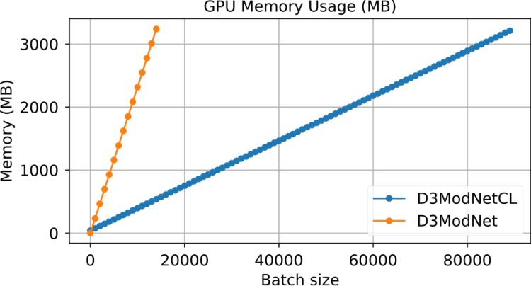
Another interesting observation can be done if we analyze Fig. 1 alongside Fig. 10. The GPU used has GB of memory. As one may notice in Fig. 10, D3ModNet’s memory usage line has a higher slope when compared to D3ModNetCL. As a result, the approach based on non-associative layers consumes the full GPU memory quickly. In contrast, the ConformalLayers-based approach supports larger batches before using all the memory. It is because the feature map resulting from each operation in D3ModNet has to be stored in memory to be passed as input to the next operation. Hence, D3ModNet’s curve in Fig. 1 shows that the maximum batch size for this architecture in this GPU is K, while the D3ModNetCL supports up to K images simultaneously.
We used linear regression in Fig. 1 to extrapolate the memory bottleneck of D3ModNet and estimate its inference time with more than K images. The extrapolation allows the comparison of both approaches under the maximum capacity of D3ModNetCL. Fig. 1 shows that our approach is about times faster than the non-associative CNN. Such improvement and memory saving suggest that the presented technique is feasible for devices with limited capabilities.
V Conclusions and Future Work

We presented the ReSPro, a novel non-linear and differentiable activation function that can be fully encoded as matrices and rank- tensors, whose product satisfies the associative law. In our experiments, we did not notice ReSPro suffering from vanishing or exploding gradient, like other S-shaped functions, probably because it behaves like element-wise activation followed by normalization instead of performing simple element-wise transformations. We also presented a new neural network back end called ConformalLayers. To the best of our knowledge, ConformalLayers is the first non-linear sequential CNN with associative layers. The combination of layers by associativity has several advantages in terms of computational efficiency during inference.
The current implementation of ConformalLayers does not support channel groups nor bias in convolutions, and does not implement transposed convolution and fully connected layers. We are working on adding these features to our framework.
Although this paper presents ConformalLayers as an architecture for sequential CNNs, we believe that we can expand the concept to non-sequential networks. One possibility is, before inference, to traverse the graph defined by the layers of non-sequential CNNs in a depth-first fashion and apply the associativity of the ConformalLayers to the paths found.
We hope that our original ideas lead to new lines of investigation. Possible directions of future exploration include the proposition of other activation functions, and the study of the data encoded by the matrix and rank- tensor .
Acknowledgments
This work was partially supported by CNPq (311.037/2017-8) and FAPERJ (E-26/202.718/2018) agencies.
References
- [1] E. L. Denton, W. Zaremba, J. Bruna, Y. LeCun, and R. Fergus, “Exploiting linear structure within convolutional networks for efficient evaluation,” in NeurIPS, 2014, pp. 1269–1277.
- [2] I. Hubara, M. Courbariaux, D. Soudry, R. El-Yaniv, and Y. Bengio, “Binarized neural networks,” in NeurIPS, 2016, pp. 4114–4122.
- [3] ——, “Quantized neural networks: training neural networks with low precision weights and activations,” J. Mach. Learn. Res., vol. 18, no. 1, pp. 6869–6898, 2017.
- [4] J. Frankle and M. Carbin, “The lottery ticket hypothesis: finding sparse, trainable neural networks,” in ICLR, 2019, pp. 1–13.
- [5] H. Zhou, J. Lan, R. Liu, and J. Yosinski, “Deconstructing lottery tickets: zeros, signs, and the supermask,” in NeurIPS, 2019, pp. 3592–3602.
- [6] H. Omidvar, V. Akhlaghi, H. Su, M. Franceschetti, and R. Gupta, “Associative convolutional layers,” in AISTATS, 2021, pp. 3115–3123.
- [7] M. Alwani, H. Chen, M. Ferdman, and P. Milder, “Fused-layer CNN accelerators,” in MICRO, 2016, pp. 1–12.
- [8] A. G. Howard, M. Zhu, B. Chen, D. Kalenichenko, W. Wang, T. Weyand, M. Andreetto, and H. Adam, “Mobilenets: efficient convolutional neural networks for mobile vision applications,” arXiv: 1704.04861, 2017.
- [9] M. Tan and Q. Le, “Efficientnet: rethinking model scaling for convolutional neural networks,” in ICML, 2019, pp. 6105–6114.
- [10] O. Saha, A. Kusupati, H. V. Simhadri, M. Varma, and P. Jain, “RNNPool: efficient non-linear pooling for RAM constrained inference,” in NeurIPS, 2020, pp. 20 473–20 484.
- [11] I. Goodfellow, Y. Bengio, and A. Courville, Deep Learning. MIT, 2016.
- [12] R. H. Hahnloser, R. Sarpeshkar, M. A. Mahowald, R. J. Douglas, and H. S. Seung, “Digital selection and analogue amplification coexist in a cortex-inspired silicon circuit,” Nature, vol. 405, no. 6789, p. 947, 2000.
- [13] D. Hendrycks and K. Gimpel, “Gaussian error linear units (GELUs),” arXiv: 1606.08415, 2016.
- [14] P. Ramachandran, B. Zoph, and Q. V. Le, “Swish: a self-gated activation function,” arXiv: 1710.05941, 2017.
- [15] I. V. Tetko, “Associative neural network,” Neural Process. Lett., vol. 16, no. 2, pp. 187–199, 2002.
- [16] J. Redmon, S. Divvala, R. Girshick, and A. Farhadi, “You only look once: unified, real-time object detection,” in CVPR, 2016, pp. 779–788.
- [17] B. Wu, F. Iandola, P. Jin, and K. Keutzer, “Squeezedet: unified, small, low power fully convolutional neural networks for real-time object detection for autonomous driving,” in CVPR Workshops, 2017, pp. 129–137.
- [18] L. Dorst, D. Fontijne, and S. Mann, Geometric algebra for computer science: an object-oriented approach to geometry. Elsevier, 2010.
- [19] R. C. Gonzalez and R. E. Woods, Digital image processing, 3rd ed. Pearson, 2008.
- [20] W. H. Young, “On the multiplication of successions of Fourier constants,” Proc. R. Soc. Lond. Series A, Containing Papers of a Mathematical and Physical Character, vol. 87, no. 596, pp. 331–339, 1912.
- [21] J. Bergstra, D. Yamins, and D. Cox, “Making a science of model search: hyperparameter optimization in hundreds of dimensions for vision architectures,” in ICML, 2013, pp. 115–123.
- [22] L. Li, K. Jamieson, G. DeSalvo, A. Rostamizadeh, and A. Talwalkar, “Hyperband: a novel bandit-based approach to hyperparameter optimization,” J. Mach. Learn. Res., vol. 18, no. 1, pp. 6765–6816, 2017.
- [23] Y. Lecun, L. Bottou, Y. Bengio, and P. Haffner, “Gradient-based learning applied to document recognition,” Proc. IEEE, vol. 86, no. 11, pp. 2278–2324, 1998.