ReLAX: Reinforcement Learning Agent eXplainer for Arbitrary Predictive ModelsDOI: XXXXXXX.XXXXXXXConference: Make sure to enter the correct conference title from your rights confirmation emai; June 03–05, 2018; Woodstock, NYPrice: 15.00ISBN: 978-1-4503-XXXX-X/18/06CCS: Computing methodologies Reinforcement learningCCS: Computing methodologies Sequential decision makingCCS: Computing methodologies Machine learningCCS: Computing methodologies Artificial intelligence
Abstract.
Counterfactual examples (CFs) are one of the most popular methods for attaching post-hoc explanations to machine learning (ML) models. However, existing CF generation methods either exploit the internals of specific models or depend on each sample’s neighborhood, thus they are hard to generalize for complex models and inefficient for large datasets. This work aims to overcome these limitations and introduces ReLAX, a model-agnostic algorithm to generate optimal counterfactual explanations. Specifically, we formulate the problem of crafting CFs as a sequential decision-making task and then find the optimal CFs via deep reinforcement learning (DRL) with discrete-continuous hybrid action space. Extensive experiments conducted on several tabular datasets have shown that ReLAX outperforms existing CF generation baselines, as it produces sparser counterfactuals, is more scalable to complex target models to explain, and generalizes to both classification and regression tasks. Finally, to demonstrate the usefulness of our method in a real-world use case, we leverage CFs generated by ReLAX to suggest actions that a country should take to reduce the risk of mortality due to COVID-19. Interestingly enough, the actions recommended by our method correspond to the strategies that many countries have actually implemented to counter the COVID-19 pandemic.
Keywords:
machine learning explainability, explainable AI, counterfactual explanations, deep reinforcement learning.1. Introduction
Recent years have witnessed surprising advances in machine learning (ML), which in turn have led to the pervasive application of ML models across several domains. Unfortunately, though, many ML systems deployed in the wild are treated as “black boxes”, whose complexity often hides the inner logic behind their output predictions. In fact, knowing why an ML model returns a certain output in response to a given input is pivotal for a variety of reasons, such as model debugging, aiding decision-making, or fulfilling legal requirements (EU 2016).
To properly achieve model transparency, a new initiative named eXplainable AI (XAI) has emerged (Samek et al. 2019). A large body of work on XAI has flourished in recent years (Guidotti et al. 2018), and approaches to XAI can be broadly categorized into two classes (Verma et al. 2020): (i) native and (ii) post-hoc. The former leverages ML models that are inherently interpretable and transparent, such as linear/logistic regression, decision trees, association rules, etc. The latter aims at generating ex post explanations for predictions made by opaque or black-box models like random forests and (deep) neural networks.
In this work, we focus on specific post-hoc explanations called counterfactual explanations, which are used to interpret predictions of individual instances in the form: “If A had been different, B would not have occurred” (Stepin et al. 2021)(Wachter et al. 2017). They work by generating modified versions of input samples that result in alternative output responses from the predictive model, i.e., counterfactual examples (CFs).
Typically, the problem of generating CFs is formulated as an optimization task, whose goal is to find the ‘‘closest’’ data point to a given instance, which crosses the decision boundary induced by a trained predictive model.11 1 We voluntarily left this notion of “closeness” underspecified here; a more precise definition of it is provided in Section 3. Depending on the level of access to the underlying predictive model, different CF generation methods have been proposed. More specifically, we can broadly distinguish between three categories of CF generators: (i) model-specific (Kanamori et al. 2020; Karimi et al. 2020b; Karimi et al. 2020a; Russell 2019; Ustun et al. 2019), (ii) gradient-aware (Wachter et al. 2017; Pawelczyk et al. 2020), and (iii) model-agnostic (Dandl et al. 2020). In short, existing CF generators require complete knowledge of the model’s internals (e.g., random forests or neural networks), or they work only with differentiable models, or finally, they depend on each sample’s neighborhood. Thus, they are hard to generalize for more complex models and inefficient for large datasets.
To overcome these limitations, we introduce a novel CF generation method called ReLAX. Specifically, we formulate the problem of crafting CFs as a sequential decision-making task. We then find the optimal CFs via deep reinforcement learning (DRL). The intuition behind ReLAX is the following. The transformation of a given input instance into its optimal CF can be seen as the sequence of actions that an agent must take in order to get the maximum expected reward (i.e., the optimal policy). The total expected reward considers both the desired CF prediction goal (i.e., the CF and the original sample must result in different responses when they are input to the predictive model) and the distance of the generated CF from the original instance. At each time step, the agent has either achieved the desired CF transformation or it needs to: (i) select a feature to modify and (ii) set the magnitude of such change. To generate meaningful CFs, the agent must restrict itself to operate on the set of actionable features only, as not every input feature can always be changed (e.g., the “age” of an individual cannot be modified). Moreover, even if actionable, some features can only be changed toward one direction (e.g., a person can only increase their “educational level”). Plus, the total number of tweaked features, as well as the magnitude of the change, must also be limited, as this would likely result in a more feasible CF. We show that solving the constrained objective to find the optimal CF generator is equivalent to learning the optimal policy of a DRL agent operating in a discrete-continuous hybrid action space.
Our proposed method is a model-agnostic CF generator, as it can be applied to any black-box predictive model. Indeed, in our framework the predictive model is just a “placeholder” resembling the environment which the DRL agent interacts with.
We validate our method on five datasets (four of them used for classification and one for regression), and compare it against several baselines using four standard quality metrics. Experimental results show that ReLAX outperforms all the competitors in every single metric. To further demonstrate the impact of our CF generation method in practice, we show that CFs generated by ReLAX can be leveraged to suggest actions that a country should take to reduce the risk of mortality due to the COVID-19 pandemic.
Overall, the main contributions of this work are as follows:
- •
ReLAX is the first method for generating model-agnostic counterfactual examples based on deep reinforcement learning. It is scalable with respect to the number of features and instances. It can explain any black-box model trained on tabular input data, regardless of its internal complexity and prediction task (classification or regression).
- •
We implement two variants of our method: ReLAX-Global and ReLAX-Local, with the latter obtained via transfer learning from a pretrained version of the former. Both methods generate +60% valid CFs that are about 40% sparser than those produced by state of the art techniques yet take 42% less CF generation time.
- •
To overcome the sparse reward problem due to the large state and action space, we integrate a hierarchical curiosity-driven exploration mechanism into our DRL agent.
- •
We further assess the power of ReLAX on a real-world use case. More specifically, we show that the actions suggested by ReLAX to reduce the risk of mortality due to the COVID-19 pandemic correspond to the strategies that many countries have actually put in practice.
- •
The source code implementation of ReLAX and the datasets (including the one used for the COVID-19 risk of mortality task) are made publicly available.22 2 https://github.com/Mewtwo1996/ReLAX.git
The remainder of the paper is organized as follows. In Section 2, we review related work. In Section 3, we formalize the problem of generating counterfactual explanations, while in Section 4 we present ReLAX, our proposed method to solve this problem using deep reinforcement learning. We validate our approach and discuss the main findings of our work in Section 5. In Section 6, we further demonstrate the practical impact of ReLAX on a real-world use case. Finally, Section 7 concludes the paper.
2. Related Work
2.1. Counterfactual Explanations for Machine Learning Predictions
A comprehensive review of the most relevant work in this area can be found in (Verma et al. 2020)(Guidotti 2022)(Wang et al. 2021)(Poyiadzi et al. 2020)(Lucic et al. 2022b). A possible approach to counterfactual explanation is called Nearest-CT (Le et al. 2020). Instead of generating a synthetic CF for a given input sample, this approach selects the nearest CF data point from the training set. More sophisticated counterfactual explanation methods can be broadly classified into model-specific and model-agnostic; as the names suggest, the former are tailored for a particular ML model (e.g., random forest), whereas the latter are able to generate explanations for any model.
Model-specific. One of the first counterfactual explanation method – FeatTweak – is proposed by Tolomei et al. (Tolomei et al. 2017), which is specifically designed for random forests, and exploits the internal structure of the learned trees to generate synthetic counterfactual instances. Another approach that is conceived for explaining tree ensembles is called FOCUS (Lucic et al. 2022a). It frames the problem of finding counterfactual explanations as an optimization task and uses probabilistic model approximations in the optimization framework. Meanwhile, the rise of deep learning has given way to more complex and opaque neural networks (NNs). In this regard, DeepFool (Moosavi-Dezfooli et al. 2016) – which was originally designed for crafting adversarial examples to undermine the robustness of NNs – has proven effective also as a CF generation method. However, CFs obtained from adversarial techniques often require changing almost all the features of the original instances, making them unrealistic to implement. Thus, Le et al. (Le et al. 2020) propose GRACE: a novel technique that explains NN model’s predictions using sparser CFs, which therefore are suitable also for high-dimensional datasets.
Model-agnostic. Guidotti et al. (Guidotti et al. 2018) introduce LORE, which first trains an interpretable surrogate model on a synthetic sample’s neighborhood generated by a genetic algorithm. Then, LORE derives an explanation consisting of a decision rule and a set of counterfactual rules. More recently, Karimi et al. (Karimi et al. 2020a) propose MACE, which frames the generation of model-agnostic CFs into solving a sequence of satisfiability problems, where both the distance function (objective) and predictive model (constraints) are represented as logic formulae. In addition, Mothilal et al. (Mothilal et al. 2020) present DiCE, a framework for generating and evaluating a diverse and feasible set of counterfactual explanations, which assumes knowledge of the model’s gradients is available, thus not fully model-agnostic.
Our ReLAX method is totally model-agnostic and aims to be as general and flexible as possible. Moreover, different from existing model-agnostic methods, ReLAX is much more efficient to generate optimal CFs. Indeed, ReLAX requires to train a DRL agent that makes use only of the input/output nature of the target predictive model to explain, regardless of its internal complexity or its gradients (as opposed to DiCE). Our method better scales to high-dimensional, large datasets than LORE: the genetic algorithm used to build each synthetic sample’s neighborhood may be unfeasible for large feature spaces. Plus, LORE also requires to train a locally-interpretable decision tree that is tight to each generated neighborhood, and therefore may be prone to overfitting. ReLAX can also seamlessly handle more complex models than MACE (e.g., deeper NNs), which needs to construct a first-order logic characteristic formula from the predictive model and test for its satisfiability. This may be intractable when the formula (i.e., the model to explain) is too large. Finally, in contrast with ReLAX, both LORE and MACE do not consider nor control over the sparsity of the generated CFs; moreover, LORE does not even take into account their actionability.
2.2. Reinforcement Learning with Parameterized Action Space
Many real-world reinforcement learning (RL) problems requires complex controls with discrete-continuous hybrid action space. For example, in Robot Soccer (Masson et al. 2016), the agent not only needs to choose whether to shoot or pass the ball (i.e., discrete actions) but also the associated angle and force (i.e., continuous parameters). Unfortunately, most conventional RL algorithms cannot deal with such a heterogeneous action space directly. The straightforward methods either discretize the continuous action space into a large discrete set (Sherstov and Stone 2005), or convert a discrete action into a continuous action method (Hausknecht et al. 2016), but they significantly increase the problem complexity. To overcome this issue, a few recent works propose to learn RL policies over the original hybrid action space directly. Specifically, they consider a parameterized action space containing a set of discrete actions and corresponding continuous action-parameter . In this way, the action space can be represented as: Masson et al. (Masson et al. 2016) propose a learning framework Q-PAMDP that alternatively learns the discrete action selection via -learning and employs policy search to get continuous action-parameters. Following the idea of Q-PAMDP, Khamassi et al. (Khamassi et al. 2017) treat two actions separately. The only difference is that they use policy gradient to optimize the continuous parameters. Both methods are on-policy and assume that continuous parameters are normally distributed. Also, Wei et al. (Wei et al. 2018) propose a hierarchical approach to deal with the parameterized action space, where the parameter policy is conditioned on the discrete policy. Although efficient, this method is found to be unstable due to its joint-learning nature. Recently, in order to avoid approximation as well as reduce complexity, Xiong et al. (Xiong et al. 2018) introduce P-DQN, which seamlessly combines and integrate both DQN (Mnih et al. 2013) and DDPG (Lillicrap et al. 2016). Empirical study indicates that P-DQN is efficient and robust.
3. Problem Formulation
Let be an input feature space and an output label space. Without loss of generality, we consider both the -ary classification setting, i.e., , and the regression setting, i.e., . Suppose there exists a predictive model , parameterized by , which accurately maps any input feature vector to its label .
The idea of counterfactual explanations is to reveal the rationale behind predictions made by on individual inputs by means of counterfactual examples (CFs). More specifically, for an instance , a CF according to is found by perturbing a subset of the features of , chosen from the set . The general goal of such modification is to transform into so to change the original prediction, i.e., (Wachter et al. 2017). In particular, this depends on whether is a classifier or a regressor. In the former case, the objective would be to transform into so to change the original predicted class into another , such that . Notice that can be either specified upfront (i.e., targeted CF) or it can be any (i.e., untargeted CF). In the case is a regressor, instead, the goal is trickier: one possible approach to specifying the validity of a counterfactual example is to set a threshold and let . However, CFs found via such a thresholding are sensitive to the choice of (Spooner et al. 2021).
Either way, as long as the CF classification or regression goal is met, several CFs can be generally found for a given input . This may lead to a situation where many CFs are in fact unrealistic or useless, as they are too far from the original instance. Therefore, amongst all the possible CFs, we search for the optimal as the “closest” one to . Intuitively, this is to favor CFs that require the minimal perturbation of the original input.
More formally, let be a counterfactual generator, parameterized by , that takes as input and produces as output a counterfactual example . For a given sample of i.i.d. observations drawn from a probability distribution, i.e., , we can measure the cost of generating CFs with for all the instances in , using the following counterfactual loss function:
| (1) |
The first component () penalizes when the CF prediction goal is not satisfied. Let be the set of inputs which do not meet the CF prediction goal, e.g., in the case of classification, . Hence, we can compute as follows:
| (2) |
where is the well-known 0-1 indicator function, which evaluates to 1 iff , 0 otherwise.
The second component is any arbitrary distance function that discourages to be too far away from . For example, , where is the -norm. In this work, inspired by previous approaches, we set equal to -norm (Guidotti et al. 2018).
In addition, serves as a scaling factor to trade off between and . Notice, though, that not every input feature can be lightheartedly modified to generate a valid CF, either because it is strictly impossible to do it (e.g., the “age” of an individual cannot be changed), and/or due to ethical concerns (e.g., the “race” or the “political tendency” of a person). Therefore, we must restrict to the set of actionable features only. Plus, the total number of perturbed features must also be limited, i.e., for some value .
Eventually, we can find the optimal CF generator as the one whose parameters minimize Equation 1, i.e., by solving the following constrained objective:
| (3) | ||||
This in turn allows us to generate the optimal CF for any , as . Finally, the resulting optimal counterfactual explanation can be simply computed as (Tolomei and Silvestri 2021). The overview of a generic counterfactual explanation framework is shown in Figure 1.

4. Proposed Framework: ReLAX
In this work, we propose to find the optimal CF generator for any arbitrary model – i.e., to solve the constrained optimization problem defined in Equation 3 – via deep reinforcement learning (DRL). We call our method Reinforcement Learning Agent eXplainer (ReLAX).
4.1. Markov Decision Process Formulation
We consider the problem of computing the optimal counterfactual example from – i.e., the optimal CF generator defined in Equation 3 – as a sequential decision-making task. More precisely, we refer to the standard reinforcement learning setting, where at each time step an agent: (i) takes an action (i.e., selects a feature of the original sample to tweak and the magnitude of such change) and (ii) receives an observation (i.e., the prediction output by on the input just modified according to the action taken before) along with a scalar reward from the environment. The process continues until the agent eventually meets the specified CF prediction goal and the optimal CF is found.
We formulate this process as a standard Markov Decision Process (MDP) . In the following, we describe each component of this framework, separately.
4.1.1. States ()
At each time step , the agent’s state is , where represents the current modified sample along with the set of features changed so far (). More specifically, is an -dimensional binary indicator vector, where iff the actionable feature has been modified in one of the actions taken by the agent before time . Initially, when , and .
If the prediction goal is met, e.g., , the agent reaches the end of the episode and the process terminates returning as the CF for . Otherwise, the agent must select an action to: (i) pick a feature to change amongst those which have not been modified yet and (ii) decide the magnitude of that change.
4.1.2. Discrete-Continuous Hybrid Actions ()
To mimic the two-step behavior discussed above, we consider a discrete-continuous hybrid action space with a two-tier hierarchical structure.
For an arbitrary step , we maintain the set of feature identifiers that the agent is allowed to modify ; initially, when , as the agent can pick any of the actionable features to change. Then, at each time step , the agent first chooses a high level action from the discrete set . This is to allow each feature to be selected at most in one action. Upon choosing , the agent must further select a low level parameter , which specifies the magnitude of the change applied to feature . It is worth noticing that we can confine the action’s range and direction by directly putting a constraint on the low level parameter . Overall, , and we define our discrete-continuous hybrid action space as follows:
4.1.3. Transition Function ()
Let be the generic action that the agent can take at time . The action deterministically moves the agent from state to state , by operating on and as follows:
| (4) |
The statements and are shorthand for and , respectively. This corresponds to increasing the value of feature by the magnitude , and updating the binary indicator vector accordingly.
4.1.4. Reward ()
The reward is expressed in terms of the objective function defined in Equation 3 and has the following form:
| (5) |
where and is a parameter that controls how much weight to put over the distance between the current modified instance () and the original sample (). In other words, the agent aims to reach a trade-off between achieving the CF prediction goal and keeping the distance of the counterfactual from the original input sample as lower as possible.
4.1.5. Policy ()
We define a parameterized policy to maximize the expected reward in the MDP problem. Our ultimate goal, though, is to find an optimal policy that solves Equation 3. It is worth noticing that finding the optimal policy that maximizes the expected return in this environment is equivalent to minimizing Equation 1, and thereby finding the optimal CF generator . The equivalence between these two formulations is shown below:
Here, defines the maximum steps taken by the agent for each sample and is set to 50,000.
4.2. Policy Optimization
We use the P-DQN framework (Xiong et al. 2018) to find the optimal policy . At each time step, the agent takes a hybrid action to perturb the currently modified , obtained from the original input .

In -learning, one aims at finding the optimal -value function representing the expected discounted reward for taking action at a given state . Inside the -value function, the continuous parameter is associated with the discrete action , which means is the optimal action given state and : . We therefore cast this as a function . Thus, the Bellman equation can be written as:
As with DQN, a deep neural network (DNN) is used to approximate the -value function, and we fit with another deterministic policy network , where and are the parameters of the two DNNs. To find the optimal , we minimize the loss functions below via stochastic gradient descent:
where the is the n-step target (Sutton and Barto 1998). Theoretically, as the error diminishes, the network converges to the optimal -value function and the policy network outputs the optimal continuous action. However, this method is unstable in practice. This is because DQN only samples transition pairs uniformly from the replay buffer. Therefore, we adopt prioritized experience replay (Schaul et al. 2015) to effectively learn from pairs with high expected learning value. As a measurement for learning potential, prioritized experience replay samples transition pairs with probability based on their TD error: , where is a parameter to determine how much prioritization is used. During training, the transition pairs are stored in the replay buffer with their priority; a sum tree data structure is then used to efficiently update the priority and sample pairs from the replay buffer.
4.3. Hierarchical Curiosity-Driven Exploration
In the procedure of generating counterfactual examples, the sparse reward problem is inevitably met due to the large state and action space. Reward shaping is a typical solution that converts the sparse reward to a dense one (Hu et al. 2020)(Grzes and Kudenko 2009); however, it is hard to design the intermediate rewards for all black box models. Hence, we develop a hierarchical curiosity-driven exploration mechanism to P-DQN.
Specifically, we adopt a Random Network Distillation (RND) module (Burda et al. 2018), i.e., a curiosity-driven approach to generate state curiosity by quantifying the next-state novelty, which will be further combined with the external rewards to generate the modified reward . RND transforms the exploring procedure into a supervised learning task by minimizing the mean squared error:
where is the fixed target network and is a trainable predictor network learning to distill the target network. The loss of trained input state () will decrease as the frequency of visited states increases; therefore, of novel states are expected higher.
Considering that the bonus is obtained after reaching the next state and will be combined with the environment reward, the agent tends to follow the existing experiences rather than keeps exploring unknown states by taking various actions. To encourage the exploration of different actions at each state, we introduce the RND module to reflect the frequency of each action. At state , the curiosity of a hybrid action is given by:
where and have the same role as and , respectively.
Here, we leverage state curiosity to enhance high-level index planning in discrete spaces, and is adopted as low-level action curiosity for enthusiastically searching continuous parameters. Finally, we organically incorporate the two-level curiosity loss into the loss functions defined above in Section 4.2:
It is worth remarking that is a function of . By alternatively updating and , the policy network will learn to balance the action’s potential value and novelty.
The overview of our ReLAX framework is depicted in Figure 2.
4.4. Global vs. Local Policy
So far, we have considered one single agent as responsible for generating the CFs for all the instances of a given dataset, and hereinafter we refer to it as ReLAX-Global. This allows us to learn a generalized policy that is able to produce counterfactuals, which are not tailored to a specific input sample. Algorithm 1 describes the training of ReLAX-Global with the hierarchical curiosity-driven exploration technique discussed in Section 4.3 above.
However, in some cases, the CF generation process should capture the peculiarities of each individual original instance. To accomodate such a need, we introduce a variant called ReLAX-Local.
ReLAX-Local trains a dedicated agent for crafting the optimal CF for a single target example. It starts by initializing ReLAX-Local’s policy with a pretrained ReLAX-Global’s policy. Then, using a standard transfer learning approach (Zhuang et al. 2021), ReLAX-Local is fine-tuned on the target samples. This step consists of randomly generating synthetic training data points around the target example, using a method similar to (Guidotti et al. 2018). Specifically, we uniformly sample data points whose -norm from the target example is at most .33 3 Notice that all our input samples are normalized unit vectors.
5. Experiments
5.1. Setup
Datasets and Tasks. We test with five public tabular datasets described in Table 1, used for classification and regression tasks.
| Dataset | N. of Instances | N. of Features | Task |
|---|---|---|---|
| Breast Cancer (bre 1995) | 699 | 10 (numerical) | classification |
| Diabetes (dia 1988) | 768 | 8 (numerical) | classification |
| Sonar (son 1988) | 208 | 60 (numerical) | classification |
| Wave (wav 1988) | 5,000 | 21 (numerical) | classification |
| Boston Housing (bos 1978) | 506 | 14 (mixed) | regression |
Predictive Models. Each dataset is randomly split into 70% training and 30% test portions. For each task and the associated dataset, we train the suitable set of predictive models chosen amongst the following: Random Forest (RF), Adaptive Boosting (AdaBoost), Gradient Boosting (XGBoost), Multi-Layer Perceptron (MLP), and Multi-Layer Perceptron for Regression (MLP-Reg). Both MLP and MLP-Reg are fully-connected feed-forward neural networks with two hidden layers; MLP includes also a logistic (i.e., sigmoid) activation function at the last output layer. Notice that some combinations do not apply, e.g., MLP-Reg is only trained on the Boston Housing dataset. We perform 10-fold cross validation on the training set portion of each dataset to fine-tune the hyperparameters of all the trainable models. Hence, for each task/dataset pair, we re-train all the applicable models with the best hyperparameters on the whole training set, and we measure their performance on the test set previously hold out. To assess the quality of the predictive models, we use accuracy for classification and RMSE for regression. Eventually, we consider only the best performing model(s) for each task/dataset pair. In Table 2, we summarize the main characteristics of each predictive model used in combination with the benchmarking datasets.
| Dataset [Best Model] | Structure | Acc. ()/RMSE () |
|---|---|---|
| Breast Cancer [RF] | {#trees=100} | 0.99 () |
| Diabetes [AdaBoost] | {#trees=100} | 0.79 () |
| Wave [XGBoost] | {#trees=100} | 0.95 () |
| Breast Cancer [MLP] | {#L1=64, #L2=128} | 1.00 () |
| Sonar [MLP] | {#L1=256, #L2=256} | 0.90 () |
| Wave [MLP] | {#L1=100, #L2=200} | 0.97 () |
| Boston Housing [MLP-Reg] | {#L1=50, #L2=128} | 3.36 () |
Counterfactual Generator Baselines. We compare ReLAX with all the CF generator baselines described in Section 2. Nearest-CT is considered the simplest approach. Furthermore, we distinguish between model-specific and model-agnostic methods. The former include: FeatTweak and FOCUS (tree-specific); DeepFool and GRACE (NN-specific). The latter are: LORE, MACE, and DiCE.
Methodology. We compare the set of CF generation methods that are suitable for each dataset/target model shown in Table 2. In particular, model-agnostic techniques (including both variants of our ReLAX) clearly apply to every setting, whereas model-specific approaches can be tested only when the target model matches (e.g., FOCUS can be used only in combination with tree-based models). Eventually, we generate a separate CF for each input sample in the test set of every dataset above, using all the CF generators relevant to the setting at hand, i.e., all the model-agnostic methods along with model-specific ones that apply.
Evaluation Metrics. We evaluate the quality of generated CFs according to the following four standard metrics (Verma et al. 2020): Validity, Proximity, Sparsity, and Generation Time. Validity measures the ratio of CFs that actually meet the prediction goal to the total number of CFs generated:44 4 Some work consider the complementary metric, which is known as Fidelity and is equal to (1-Validity). the higher the validity the better. Proximity computes the distance of a CF from the original input sample; in this work, we use -norm to measure proximity, and therefore the smaller it is the better. Sparsity indicates the number of features that must be changed according to a CF, and therefore is equivalent to the -norm between a CF and the corresponding original input sample. The smaller it is the better, as sparser CFs likely lead to more human-interpretable explanations. Finally, Generation Time computes the time required to generate CFs, which, clearly, should be as small as possible. All the metrics above are averaged across all the test input samples. Moreover, experiments were repeated 5 times and results are expressed as the mean standard deviation.
5.2. Results
Sparsity-Validity Trade-off. In Figure 3, we plot the number of perturbed features (i.e., sparsity) versus the validity of counterfactuals obtained with different CF generation methods, when applied to classification tasks. More specifically, we fix a threshold on the maximum number of features that each CF generator is allowed to perturb and we show: (i) the actual sparsity; and (ii) the validity of the generated CFs. The rationale of this analysis is to show which method is able to achieve the best trade-off between two contrasting metrics: sparsity and validity. Intuitively, the larger is the number of perturbed features, the higher is the chance of obtaining a valid counterfactual. On the other hand, we should privilege sparser CFs, i.e., CFs that modify as less features as possible, since those are possibly more interpretable and feasible to implement.

Results show that both ReLAX-Global and ReLAX-Local achieve the best balance between sparsity and validity. That is, our method outperforms all the baselines in terms of validity and, more importantly, it obtains these results even when we set a very restrictive threshold on sparsity, i.e., when few features are modified. As expected, though, if we soften such a cap on the number of features allowed to change, other methods like LORE may eventually match the performance of ReLAX or even reach higher validity scores. In fact, not controlling for sparsity will make all CF generation methods behave similarly. This is what we observe when we test with DeepFool or the simplest Nearest-CT baseline, which by design tend to generate valid CFs only if a large fraction of the input features get modified. Due to this behavior, both DeepFool and Nearest-CT cannot be visualized in the plots, as they fall outside the range of sparsity values imposed in our experiments. Furthermore, although MACE is model-agnostic, its applicability to neural network target models is problematic due to its large computational cost (Karimi et al. 2020a). Besides, the only implementation of MACE remaining available works only in combination with RF target models, and this is why we used it only in the first setting (Breast Cancer [RF]).
A similar analysis on the sparsity vs. validity trade-off for the Boston Housing regression task is shown in Table 3. In this case, we compare only our two variants of ReLAX since none of the CF generation baselines considered is designed to operate in a regression setting. As expected, the larger is the tolerance used to determine if the prediction goal of the counterfactual example is met the harder is for ReLAX to find a valid counterfactual.
| Validity (Sparsity) | ||
|---|---|---|
| Threshold () | ReLAX-Global | ReLAX-Local |
| 0.20 | () | () |
| 0.40 | () | () |
| 0.60 | () | () |
Finally, analogous conclusions can be drawn if we compare proximity vs. validity (see Table 4): ReLAX is able to strike the best balance also between those two conflicting metrics.
Generation Time. Although validity and sparsity (proximity) are crucial to measure the quality of a CF generation method, efficiency is pivotal as well. Therefore, we compare the average generation time for each model-agnostic CF generator, namely LORE, MACE, and our ReLAX in its two variants. We focus on model-agnostic methods because we want this comparison to be as general as possible. Table 4 shows that our method takes up to 42% less time than other model-agnostic baseline to produce valid counterfactuals, which happen to be also closer to the original instances. This result is even more remarkable if we consider that the counterfactual generation time of ReLAX includes the training of the DRL agent.
| Metric | Dataset [Models] | CF Generation Methods | |||
| ReLAX-Global | ReLAX-Local | LORE | MACE | ||
| Proximity | Breast Cancer [RF, MLP] | [] | [] | [] | [, N/A] |
| Diabetes [AdaBoost] | [] | [] | [] | [N/A] | |
| Sonar [MLP] | [] | [] | [] | [N/A] | |
| Wave [XGBoost, MLP] | [] | [] | [] | [N/A, N/A] | |
| Boston Housing [MLP-Reg] | [] | [] | [N/A] | [N/A] | |
| Generation Time (secs.) | * | ||||
5.3. Hyperparameter Tuning
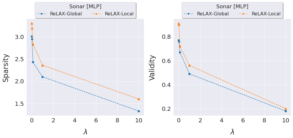
Our CF generation method is associated with a number of controlling parameters. To understand the impact of these parameters, we analyze the behavior of ReLAX on the Sonar dataset with MLP as the target classifier and the maximal sparsity limited to 5 features.
The scaling factor . We first investigate the effect of the scaling factor on the generated CFs, picking it from . As shown in Figure 4, controls the balance between sparsity and validity. Indeed, larger values of force the agent to prefer sparser CFs at the expense of lower validity (see Figure 4 – left), whereas smaller values of result in the opposite (see Figure 4 – right).
The target model’s architecture. We assess the robustness of our CF generation method when applied to different target neural network architectures. More specifically, Table 5 shows the impact of different MLP architectures on the validity and sparsity of counterfactuals generated by ReLAX in comparison with two competitors: GRACE (NN-specific) and LORE (model-agnostic).
| Validity (Sparsity) | |||||
|---|---|---|---|---|---|
| MLP size | Acc. | ReLAX-Global | ReLAX-Local | GRACE | LORE |
| [256, 256] | () | () | () | () | |
| [128, 128] | () | () | () | () | |
| [64, 64] | () | () | () | () | |
We may observe that both GRACE and LORE are quite sensitive to the MLP size, i.e., when the target neural network is getting large the validity and sparsity of CFs generated with those two methods deteriorate significantly. In the case of GRACE, the reason for that detrimental effect is due to the fact that it leverages the gradient of the function approximated by the neural network, which is obviously correlated with the complexity of the MLP structure. Despite model-agnostic, LORE requires to accurately learn a locally-interpretable surrogate model of the target neural network, which may be hard when this becomes too complex. Instead, ReLAX is more robust toward different MLP structures, and its performance is consistent independently of the MLP size. Indeed, the agent underneath ReLAX truly treats the target model as a black box regardless of its internal complexity.
The efficiency of pretraining. Finally, we show how pretrained ReLAX-Global improves the performance of ReLAX-Local. More specifically, we train ReLAX-Local as described in Section 4.4, and compare it with another agent learned from scratch. Unsurprisingly, initializing ReLAX-Local with pretrained ReLAX-Global reduces its CFs generation time, as shown in Table 6.
| Setting | Validity (Sparsity) | Gen. Time (secs.) |
|---|---|---|
| without pretraining | () | |
| with pretraining | () |
6. Case Study: COVID-19 Mortality
The goal of this case study is to demonstrate that counterfactual explanations provided by ReLAX may help countries that suffer from high COVID-19 mortality taking effective actions, economically and medically, to reduce such risk.
To achieve that, we first need to learn a binary classifier that predicts whether the country’s death risk due to COVID-19 is high or not, given the country-level features. Inspired by previous work addressing a similar task (Bird et al. 2020), we gather 17 country-level demographic features from 156 countries across 7 continents (Worldometers 2013; Central Intelligency Agency 2020; World Health Organization 2020; World Health Organization 2017). Furthermore, we label each instance with a binary class denoting the COVID-19 risk of mortality (“high” vs. “normal”), as in (Bird et al. 2020). This dataset is made publicly available.55 5 https://github.com/Mewtwo1996/ReLAX.git
We randomly split our collected dataset into two parts, i.e., used for training and for test. Therefore, we train the following models to learn the binary classifier for predicting COVID-19 mortality risk: SVM, RF, AdaBoost, and XGBoost. After running 10-fold cross validation, the best-performing model turns out to be XGBoost with 500 trees, which achieves accuracy on the test set. We sort the features according to the ranking induced by the XGBoost model, as shown in Figure 5 (left). Then, we generate with our ReLAX algorithm the CFs for the 16 high-risk countries in the test set. It is worth remarking that, although the target binary classifier is learned considering all the features from the whole training set, we force ReLAX to tweak only the subset of actionable features so that effective suggestions can be found by observing the generated CFs. Besides, in order to avoid bizarre recommendations, we constrain the change of (actionable) features toward a “plausible” direction (e.g., it would not make any sense to suggest increasing the unemployment rate of a country).
The ReLAX agent tweaks 1.67 features on average, and the average proximity (i.e., -norm) between the original sample and the corresponding counterfactual example is 1.18. Figure 5 (right) shows the direction of feature changes as suggested by the CFs.
We observe that the CFs suggest five main changes: (i) Decreasing the death rate;66 6 Albeit it may sound odd, reducing the death rate can subsume a broader suggestion for improving the life quality of a country. (ii) Decreasing the unemployment rate; (iii) Increasing the nurse rate per 10,000 people; (iv) Decreasing the urban population rate; and (v) Decreasing the obesity prevalence. Not only those recommendations look sensible, as much as straightforward or even obvious, but their accuracy is also confirmed by the fact that many countries have indeed adopted similar strategies to counter the impact of COVID-19. For example, US approved the visa for more than 5,000 international nurses to strengthen the health workforce.77 7 https://www.npr.org/sections/health-shots/2022/01/06/1069369625/short-staffed-and-covid-battered-u-s-hospitals-are-hiring-more-foreign-nurses Moreover, according to the investigation made by the US Center for Disease Control and Prevention,88 8 https://www.cdc.gov/obesity/data/obesity-and-covid-19.html obese patients with COVID-19 aged 18 years and younger are associated with a 3.07 times higher risk of hospitalization and a 1.42 times higher risk of severe illness. Thus, reducing the obesity prevalence can indeed lower mortality risk. Finally, reducing the unemployment rate and the urban population rate may allow a broader range of people to enhance their social community awareness, take consciousness of the risks of the pandemic, and thus adopt a safe lifestyle.

7. Conclusion and Future Work
In this work, we presented ReLAX, the first method for generating model-agnostic counterfactual examples based on deep reinforcement learning with hierarchical curiosity-driven exploration. We implemented two variants of it: ReLAX-Global and ReLAX-Local. The former learns a generalized agent’s policy from a whole set of training instances, whereas the latter trains a dedicated agent’s policy for crafting the optimal counterfactual of a single target example via transfer learning from a pretrained ReLAX-Global. Extensive experiments run on five public tabular datasets demonstrated that ReLAX significantly outperforms all the considered CF generation baselines in every standard quality metric. Our method is scalable with respect to the number of features and instances, and can explain any black-box model, regardless of its internal complexity and prediction task (i.e., classification or regression). Finally, we show that CFs generated by ReLAX are useful in practice, as they can be used to suggest actions that a country should take to reduce the risk of COVID-19 mortality.
Several research directions are worth exploring in future work. For example: extend ReLAX to generate explanations for non-tabular input data like images, and compare our method against non-counterfactual explanation approaches like SHAP (Lundberg and Lee 2017) or LIME (Ribeiro et al. 2016).
Acknowledgements.
This research was supported by the Italian Ministry of Education, University and Research (MIUR) under the grant "Dipartimenti di eccellenza 2018-2022" of the Department of Computer Science and the Department of Computer Engineering at Sapienza University of Rome.References
- (1)
- bos (1978) 1978. Boston Housing Dataset. [Online]. Available from: https://www.kaggle.com/vikrishnan/boston-house-prices.
- dia (1988) 1988. Diabetes Dataset. [Online]. Available from: https://www.kaggle.com/uciml/pima-indians-diabetes-database.
- son (1988) 1988. Sonar Dataset. [Online]. Available from: https://archive.ics.uci.edu/ml/datasets/connectionist+bench+(sonar,+mines+vs.+rocks).
- wav (1988) 1988. Wave Dataset. [Online]. Available from: https://archive.ics.uci.edu/ml/datasets/waveform+database+generator+(version+1).
- bre (1995) 1995. Breast Cancer Dataset. [Online]. Available from: https://archive.ics.uci.edu/ml/datasets/breast+cancer+wisconsin+(diagnostic).
- Bird et al. (2020) Jordan J. Bird, Chloe M. Barnes, Cristiano Premebida, Anikó Ekárt, and Diego R. Faria. 2020. Country-level Pandemic Risk and Preparedness Classification based on COVID-19 Data: A Machine Learning Approach. PLoS One 15, 10 (2020).
- Burda et al. (2018) Yuri Burda, Harrison Edwards, Amos Storkey, and Oleg Klimov. 2018. Exploration by Random Network Distillation. arXiv preprint arXiv:1810.12894 (2018).
- Central Intelligency Agency (2020) Central Intelligency Agency. 2020. The CIA World Factbook2020.
- Dandl et al. (2020) Susanne Dandl, Christoph Molnar, Martin Binder, and Bernd Bischl. 2020. Multi-Objective Counterfactual Explanations. In Proc. of PPSN (Lecture Notes in Computer Science, Vol. 12269), Thomas Bäck, Mike Preuss, André H. Deutz, Hao Wang, Carola Doerr, Michael T. M. Emmerich, and Heike Trautmann (Eds.). Springer, 448–469. https://doi.org/10.1007/978-3-030-58112-1_31
- EU (2016) EU. 2016. Regulation (EU) 2016/679 of the European Parliament (GDPR). Official Journal of the European Union L119 (2016), 1–88.
- Grzes and Kudenko (2009) Marek Grzes and Daniel Kudenko. 2009. Theoretical and Empirical Analysis of Reward Shaping in Reinforcement Learning. In 2009 International Conference on Machine Learning and Applications. IEEE, 337–344.
- Guidotti (2022) Riccardo Guidotti. 2022. Counterfactual Explanations and How to Find Them: Literature Review and Benchmarking. Data Mining and Knowledge Discovery (2022), 1–55.
- Guidotti et al. (2018) Riccardo Guidotti, Anna Monreale, Salvatore Ruggieri, Dino Pedreschi, Franco Turini, and Fosca Giannotti. 2018. Local Rule-Based Explanations of Black Box Decision Systems. arXiv preprint arXiv:1805.10820 (2018).
- Hausknecht et al. (2016) Matthew Hausknecht, Prannoy Mupparaju, Sandeep Subramanian, Shivaram Kalyanakrishnan, and Peter Stone. 2016. Half Field Offense: An Environment for Multiagent Learning and Ad Hoc Teamwork. In Proc. of ALA Workshop.
- Hu et al. (2020) Yujing Hu, Weixun Wang, Hangtian Jia, Yixiang Wang, Yingfeng Chen, Jianye Hao, Feng Wu, and Changjie Fan. 2020. Learning to Utilize Shaping Rewards: A New Approach of Reward Shaping. Advances in Neural Information Processing Systems 33 (2020), 15931–15941.
- Kanamori et al. (2020) Kentaro Kanamori, Takuya Takagi, Ken Kobayashi, and Hiroki Arimura. 2020. DACE: Distribution-Aware Counterfactual Explanation by Mixed-Integer Linear Optimization. In Proc. of IJCAI, Christian Bessiere (Ed.). ijcai.org, 2855–2862. https://doi.org/10.24963/ijcai.2020/395
- Karimi et al. (2020a) Amir-Hossein Karimi, Gilles Barthe, Borja Balle, and Isabel Valera. 2020a. Model-Agnostic Counterfactual Explanations for Consequential Decisions. In Proc. of AISTATS, Silvia Chiappa and Roberto Calandra (Eds.), Vol. 108. PMLR, 895–905. http://proceedings.mlr.press/v108/karimi20a.html
- Karimi et al. (2020b) Amir-Hossein Karimi, Bodo Julius von Kügelgen, Bernhard Schölkopf, and Isabel Valera. 2020b. Algorithmic Recourse Under Imperfect Causal Knowledge: A Probabilistic Approach. In Proc. of NeurIPS (NeurIPS’20), Hugo Larochelle, Marc’Aurelio Ranzato, Raia Hadsell, Maria-Florina Balcan, and Hsuan-Tien Lin (Eds.). https://proceedings.neurips.cc/paper/2020/hash/02a3c7fb3f489288ae6942498498db20-Abstract.html
- Khamassi et al. (2017) Mehdi Khamassi, George Velentzas, Theodore Tsitsimis, and Costas Tzafestas. 2017. Active Exploration and Parameterized Reinforcement Learning Applied to a Simulated Human-Robot Interaction Task. In 2017 First IEEE International Conference on Robotic Computing (IRC). IEEE, 28–35.
- Le et al. (2020) Thai Le, Suhang Wang, and Dongwon Lee. 2020. GRACE: Generating Concise and Informative Contrastive Sample to Explain Neural Network Model’s Prediction. In Proc. of KDD (KDD’20), Rajesh Gupta, Yan Liu, Jiliang Tang, and B. Aditya Prakash (Eds.). ACM, 238–248.
- Lillicrap et al. (2016) Timothy P. Lillicrap, Jonathan J. Hunt, Alexander Pritzel, Nicolas Heess, Tom Erez, Yuval Tassa, David Silver, and Daan Wierstra. 2016. Continuous Control with Deep Reinforcement Learning. In Proc. of ICLR (ICLR’16), Yoshua Bengio and Yann LeCun (Eds.). http://arxiv.org/abs/1509.02971
- Lucic et al. (2022a) Ana Lucic, Harrie Oosterhuis, Hinda Haned, and Maarten de Rijke. 2022a. FOCUS: Flexible Optimizable Counterfactual Explanations for Tree Ensembles. In Proc. of AAAI (AAAI’22). 5313–5322. https://doi.org/10.1609/aaai.v36i5.20468
- Lucic et al. (2022b) Ana Lucic, Maartje A. Ter Hoeve, Gabriele Tolomei, Maarten De Rijke, and Fabrizio Silvestri. 2022b. CF-GNNExplainer: Counterfactual Explanations for Graph Neural Networks. In Proc. of AISTATS (AISTATS’22, Vol. 151), Gustau Camps-Valls, Francisco J. R. Ruiz, and Isabel Valera (Eds.). PMLR, 4499–4511. https://proceedings.mlr.press/v151/lucic22a.html
- Lundberg and Lee (2017) Scott M Lundberg and Su-In Lee. 2017. A Unified Approach to Interpreting Model Predictions. In Advances in Neural Information Processing Systems 30, I. Guyon, U. V. Luxburg, S. Bengio, H. Wallach, R. Fergus, S. Vishwanathan, and R. Garnett (Eds.). Curran Associates, Inc., 4765–4774. http://papers.nips.cc/paper/7062-a-unified-approach-to-interpreting-model-predictions.pdf
- Masson et al. (2016) Warwick Masson, Pravesh Ranchod, and George Konidaris. 2016. Reinforcement Learning with Parameterized Actions. In Proc. of AAAI (AAAI’16). AAAI Press, 1934–1940.
- Mnih et al. (2013) Volodymyr Mnih, Koray Kavukcuoglu, David Silver, Alex Graves, Ioannis Antonoglou, Daan Wierstra, and Martin Riedmiller. 2013. Playing Atari with Deep Reinforcement Learning. In NIPS Deep Learning Workshop.
- Moosavi-Dezfooli et al. (2016) Seyed-Mohsen Moosavi-Dezfooli, Alhussein Fawzi, and Pascal Frossard. 2016. DeepFool: A Simple and Accurate Method to Fool Deep Neural Networks. In Proc. of CVPR (CVPR’16). IEEE Computer Society, 2574–2582. https://doi.org/10.1109/CVPR.2016.282
- Mothilal et al. (2020) Ramaravind Kommiya Mothilal, Amit Sharma, and Chenhao Tan. 2020. Explaining Machine Learning Classifiers through Diverse Counterfactual Explanations. In Proc. of FAT* (FAT*’20), Mireille Hildebrandt, Carlos Castillo, L. Elisa Celis, Salvatore Ruggieri, Linnet Taylor, and Gabriela Zanfir-Fortuna (Eds.). ACM, 607–617. https://doi.org/10.1145/3351095.3372850
- Pawelczyk et al. (2020) Martin Pawelczyk, Klaus Broelemann, and Gjergji Kasneci. 2020. Learning Model-Agnostic Counterfactual Explanations for Tabular Data. In Proc. of WWW (TheWebConf’20), Yennun Huang, Irwin King, Tie-Yan Liu, and Maarten van Steen (Eds.). ACM / IW3C2, 3126–3132. https://doi.org/10.1145/3366423.3380087
- Poyiadzi et al. (2020) Rafael Poyiadzi, Kacper Sokol, Raul Santos-Rodriguez, Tijl De Bie, and Peter Flach. 2020. FACE: Feasible and Actionable Counterfactual Explanations. In Proc. of AIES (AIES’20). 344–350.
- Ribeiro et al. (2016) Marco Tulio Ribeiro, Sameer Singh, and Carlos Guestrin. 2016. "Why Should I Trust You?": Explaining the Predictions of Any Classifier. In Proc. of KDD (KDD’16). ACM, 1135–1144. https://doi.org/10.1145/2939672.2939778
- Russell (2019) Chris Russell. 2019. Efficient Search for Diverse Coherent Explanations. In Proc. of FAT* (FAT*’19), Danah Boyd and Jamie H. Morgenstern (Eds.). ACM, 20–28. https://doi.org/10.1145/3287560.3287569
- Samek et al. (2019) Wojciech Samek, Grégoire Montavon, Andrea Vedaldi, Lars Kai Hansen, and Klaus-Robert Müller. 2019. Explainable AI: Interpreting, Explaining and Visualizing Deep Learning. Springer.
- Schaul et al. (2015) Tom Schaul, John Quan, Ioannis Antonoglou, and David Silver. 2015. Prioritized Experience Replay. arXiv preprint arXiv:1511.05952 (2015).
- Sherstov and Stone (2005) Alexander A Sherstov and Peter Stone. 2005. Function Approximation via Tile Coding: Automating Parameter Choice. In International Symposium on Abstraction, Reformulation, and Approximation. Springer, 194–205.
- Spooner et al. (2021) Thomas Spooner, Danial Dervovic, Jason Long, Jon Shepard, Jiahao Chen, and Daniele Magazzeni. 2021. Counterfactual Explanations for Arbitrary Regression Models. CoRR abs/2106.15212 (2021). https://arxiv.org/abs/2106.15212
- Stepin et al. (2021) Ilia Stepin, Jose M Alonso, Alejandro Catala, and Martín Pereira-Fariña. 2021. A Survey of Contrastive and Counterfactual Explanation Generation Methods for Explainable Artificial Intelligence. IEEE Access 9 (2021), 11974–12001.
- Sutton and Barto (1998) Richard S. Sutton and Andrew G. Barto. 1998. Reinforcement Learning: An Introduction. MIT Press. http://www.cs.ualberta.ca/˜sutton/book/the-book.html
- Tolomei and Silvestri (2021) Gabriele Tolomei and Fabrizio Silvestri. 2021. Generating Actionable Interpretations from Ensembles of Decision Trees. IEEE Transactions on Knowledge and Data Engineering 33, 4 (2021), 1540–1553. https://doi.org/10.1109/TKDE.2019.2945326
- Tolomei et al. (2017) Gabriele Tolomei, Fabrizio Silvestri, Andrew Haines, and Mounia Lalmas. 2017. Interpretable Predictions of Tree-based Ensembles via Actionable Feature Tweaking. In Proc. of KDD (KDD’17). ACM, 465–474. https://doi.org/10.1145/3097983.3098039
- Ustun et al. (2019) Berk Ustun, Alexander Spangher, and Yang Liu. 2019. Actionable Recourse in Linear Classification. In Proc. of FAT* (FAT*’19), Danah Boyd and Jamie H. Morgenstern (Eds.). ACM, 10–19. https://doi.org/10.1145/3287560.3287566
- Verma et al. (2020) Sahil Verma, John Dickerson, and Keegan Hines. 2020. Counterfactual Explanations for Machine Learning: A Review. arXiv preprint arXiv:2010.10596 (2020).
- Wachter et al. (2017) Sandra Wachter, Brent Mittelstadt, and Chris Russell. 2017. Counterfactual Explanations without Opening the Black Box: Automated Decisions and the GDPR. Harvart Journal of Law & Tech. 31 (2017), 841.
- Wang et al. (2021) Yongjie Wang, Qinxu Ding, Ke Wang, Yue Liu, Xingyu Wu, Jinglong Wang, Yong Liu, and Chunyan Miao. 2021. The Skyline of Counterfactual Explanations for Machine Learning Decision Models. In Proc. of CIKM (CIKM’21). ACM, 2030–2039.
- Wei et al. (2018) Ermo Wei, Drew Wicke, and Sean Luke. 2018. Hierarchical Approaches for Reinforcement Learning in Parameterized Action Space. In 2018 AAAI Spring Symposium Series.
- World Health Organization (2017) World Health Organization. 2017. Prevalence of Obesity among Adults.
- World Health Organization (2020) World Health Organization. 2020. Global Health Workforce Statistics.
- Worldometers (2013) Worldometers. 2013. Current World Population.
- Xiong et al. (2018) Jiechao Xiong, Qing Wang, Zhuoran Yang, Peng Sun, Lei Han, Yang Zheng, Haobo Fu, Tong Zhang, Ji Liu, and Han Liu. 2018. Parametrized Deep Q-networks Learning: Reinforcement Learning with Discrete-Continuous Hybrid Action Space. arXiv preprint arXiv:1810.06394 (2018).
- Zhuang et al. (2021) Fuzhen Zhuang, Zhiyuan Qi, Keyu Duan, Dongbo Xi, Yongchun Zhu, Hengshu Zhu, Hui Xiong, and Qing He. 2021. A Comprehensive Survey on Transfer Learning. Proc. IEEE 109, 1 (2021), 43–76. https://doi.org/10.1109/JPROC.2020.3004555