Auctions between Regret-Minimizing AgentsThanks: This work has been published in Proceedings of the ACM Web Conference 2022 (WWW’22). https://doi.org/10.1145/3485447.3512055.
Abstract
We analyze a scenario in which software agents implemented as regret-minimizing algorithms engage in a repeated auction on behalf of their users. We study first-price and second-price auctions, as well as their generalized versions (e.g., as those used for ad auctions). Using both theoretical analysis and simulations, we show that, surprisingly, in second-price auctions the players have incentives to misreport their true valuations to their own learning agents, while in first-price auctions it is a dominant strategy for all players to truthfully report their valuations to their agents.
1 Introduction
This paper deals with the following common type of scenario: several users engage in a repeated online auction, where each of them is assisted by a learning agent. A typical example is advertisers that compete for ad slots: typically, each of these advertisers enters his key parameters into some advertiser-facing website, and then this website’s “agent” participates on the advertiser’s behalf in a sequence of auctions for ad slots. Often, the auction’s platform designer provides this agent as its advertiser-facing user interface. In cases where the platform’s agent does not optimize sufficiently well for the advertiser (but rather, say, for the auctioneer), one would expect some other company to provide a better (for the advertiser) agent. A typical learning algorithm of this type will have at its core some regret-minimization algorithm [41, 11], such as “multiplicative weights” (see [2] and references therein), “online gradient descent” [73], or some variant of fictitious play [14, 63], such as “follow the perturbed leader” [39, 47]. In particular, for ad auctions, there is empirical data showing that bids are largely consistent with no-regret learning [55, 61].
While one’s first intuition would be that an auction that is well designed for “regular” users would also work well for such agent-assisted users, it turns out that this is often not the case. In this paper we study how basic auction formats perform in terms of revenue and economic efficiency when software agents are doing the repeated bidding for the users. Specifically, we assume that each of the human bidders enters his valuation into a regret-minimizing software agent, and then the agent engages in a long sequence of auctions, attempting to maximize utility for the human user. We present both simulation results and theoretical analysis for several types of auctions: first-price, second-price, and generalized first- and second-price auctions (for multiple ad slots). We study both classic regret-minimizing algorithms like multiplicative weights or follow the perturbed leader, as well as the consequences of the regret-minimization property itself.
Before presenting our results, let us say what exactly we are looking at when studying a long sequence of auctions played by software agents. While one might hope that there is some kind of convergence to fixed bids or distributions, it is well known that regret-minimization dynamics in many games need not converge [21, 42, 62, 6, 5]. For example, in our context, Figure 1(a) shows the dynamics of a simulation of a generalized first-price auction for two slots where the two bidders have the same value. (Throughout the dynamics, both agents bid nearly the same value and thus only a single bid-line is visible.) As one may clearly see, the dynamics do not converge. What we wish to study is the thing that is important to the auctioneer and to the bidders: the long-term distribution of the tuple of bids. For example, Figure 1(b) shows a density map of the empirical pair of bids in this simulation. The empirical distribution of the tuple of bids determines the average winning frequencies and prices, which in turn determine the users’ utilities and the auctioneer’s revenue over the whole sequence of auctions. While there may not always be a theoretical guarantee that this empirical distribution converges either, one may still theoretically analyze properties that it may have in various cases as well as study it through simulations.
It is well known that in any game and for any regret-minimizing dynamics the distribution of tuples of bids approaches a “coarse correlated equilibrium” [39, 41, 72, 11] (CCE), but as the space of CCEs is quite wide, this often does not suffice for an analysis of parameters of interest like the revenue or social welfare. For example, both for the first- and second-price auctions, there exist multiple (full information) CCEs, with different revenues and different social welfare [29]. One of the contributions of this work, presented in Section 4, is the identification of a refinement of the class of CCEs which we term co-undominated, to which alone a large class of regret-minimizing algorithms (“mean-based” ones, as defined in [13]) may converge in any game. In some cases this refinement suffices for an analysis, and for specific regret-minimization algorithms like multiplicative weights we may get an even finer analysis.
While there has been some work on the behavior of no-regret dynamics in auctions [22, 7, 30, 23], we do not know of previous analysis of the average utilities and revenue of standard no-regret dynamics in standard auction formats. The closest paper conceptually to ours is [30], which manages to analyze these for no-regret dynamics that are preceded by a long pure exploration phase by all agents. Here we provide theoretical analysis and simulations for standard regret-minimization algorithms (without a pre-exploration phase), sometimes getting very different results. In a companion paper [48] we discuss the convergence of regret-minimizing agents and analyze the incentives of the users of such agents in a general game-theoretic setting.


1.1 Second-Price Auctions
To demonstrate the difficulty, let us start by looking at the easiest-to-analyze auction: a second-price auction of a single item among two users. It is well known [71, 28] that such an auction is (dominant-strategy) incentive compatible, i.e., that no bidder ever has any incentive to misreport his value to the auctioneer. Such truthful bidding will result in an efficient allocation where the player with the higher value wins and pays a price equal to the value of the lower player.
So now let us look at our scenario, where the two (human) users each report their value to a software agent (one agent for each player), and then the two (software) agents repeatedly engage in auctions, each agent attempting to optimize for its own user according to the value reported to it. (We assume that each auction in the sequence is for the same type of item, and that the values of the players for this type of item are fixed and additive over the items won.) What do we expect to happen in this case? Specifically: Is it in the best interest of users to report their true values to their agents? Will the player with the higher value always win? Will he pay a price equal to the value of the lower player?
While positive answers to these three questions may seem to be trivially true, this turns out not to be the case, and only the second question gets a positive answer, while the answers to the first and third questions are negative.
Theorem 1.
For two bidders with values with multiplicative-weights agents that engage in a sequence of second-price auctions on their behalf with discrete bid levels, the distribution of bids of the high player converges to uniform in the range , while the distribution of the bids of the low player converges to a distribution that has full support on . In particular, in the limit, the high player always wins and pays an average price that is strictly less than the second price.
Figure 2(a) shows the dynamics of multiplicative-weights learning agents in a second-price auction, where the values of the two agents are and , and Figure 2(b) shows the long-term distribution of bids of each of the two agents that indeed behave as the theorem states: the high-value agent always wins – except for a small number of auctions in the initial phase – and the average price he pays is about (which is well below ). This is very much in contrast to the results of [30] that show that if we start with a sufficiently long pure exploration phase in which all agents bid uniformly, then dominant strategies are indeed reached. While the proved and observed lack of convergence to the dominant strategies may be surprising, the explanation is simple: while the dominant strategies do form a Nash equilibrium of the game, there are other (full-information) Nash equilibria of this game where the first player bids arbitrarily above the second price and the second player underbids arbitrarily.11 1 These equilibria are distinct from the known “overbidding equilibria” where the low bidder bids above the high-bidder’s value and occur even if we completely disallow our learning agents to overbid as we do in our simulations. Regret dynamics do not necessarily choose the former and so we do get some distribution over the “low revenue” equilibria.

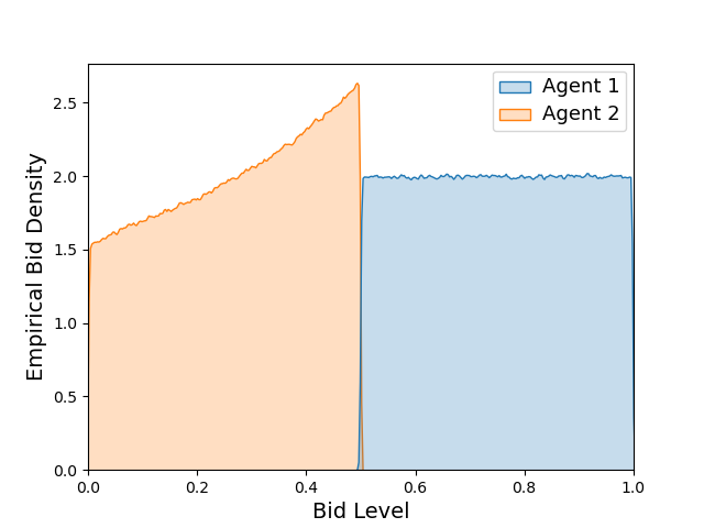

The fact that the average price paid is well below the second price has immediate implications for a human user that has a value that lies between the average price in these dynamics and the actual second price. Such a user will gain from misreporting (exaggerating) his value to his own agent. In this example, a player with value, say, that bids truthfully against a second player with value will always lose, whereas misreporting his value as will lead to these simulated dynamics (as in Figure 2), making him always win and achieve a strictly positive utility on average. One can continue this analysis, viewing the reports of the users to their own agents as defining a “meta-game” between the users, and study the reached equilibrium. In a companion paper [48], we define and study this type of “meta-game” in a general context, and in Section 5 we analyze it for the second-price auction.22 2 Spoiler: there are multiple possible equilibria in which the high player exaggerates his value as much as possible and the low player reports anything below a maximum value that is less than twice the true value of the high player.
In Appendix A.1 we also demonstrate that these types of phenomena happen not only with multiplicative-weights algorithms, but also with other classic regret-minimization learning algorithms such as “follow the perturbed leader” (FTPL). We also show in Section 5 that the same phenomena happen in a generalized second-price (GSP) auction similar to the auctions used by search engines to sell ad slots in search result web pages. One may well wonder whether the advertiser-optimizing software supplied by the search engines indeed optimizes for the advertiser (in the sense of regret minimization), and whether the search engines lose revenue by using such a generalized second-price auction.33 3 Practically, as the number of advertisers may be large, with some distribution on the participants’ values in each auction, the revenue loss should be smaller than in our simulations. Still, it is far from clear that this loss is small.
1.2 First-Price Auctions
We now turn our attention to basic first-price auctions (for a single good). What do we expect to happen in a repeated first-price auction between two regret-minimizing algorithms with values ? Our basic intuition may be that they reach some kind of (full information) equilibrium of the first-price auction. It is well known that the only pure Nash equilibrium is where the low bidder bids his value (up to an ) and the high bidder bids more than that. This means that we would expect the high player to win (almost always) and pay (close to) the second price. Mixed Nash and correlated equilibria of the first-price auction are also known to yield the same outcome (namely, the high player always wins and pays the second price) [29]. Figure 3 strengthens this intuition by showing the dynamics of first-price auctions with values and (Figure 3(a)) and with symmetric values (Figure 3(b)) between two multiplicative-weights algorithms that indeed converge to this outcome.44 4 It should be noted, though, that this convergence in the symmetric case is very slow, perhaps the slowest that we have seen in our simulations.


The missing element in this intuition is that regret-minimization dynamics need not converge to a Nash equilibrium (or even a correlated equilibrium) but may reach an arbitrary coarse correlated equilibrium, and it turns out that the first-price auction also has other coarse correlated equilibria [29], and in many of these coarse correlated equilibria the revenue is well below the second price, and sometimes even the low player wins. While in [29] these coarse correlated equilibria were analyzed in a continuous setting, they also exist with simple discrete bidding levels. For example, consider an auction with ; the reader may verify that the distribution that gives equal weights to the following four pairs of bids is a coarse correlated equilibrium: . It is true in general that for every CCE there exist some regret-minimizing algorithms that converge to it ([54], see also [48]). Specifically, in our setting, consider agents that start by playing a sequence of bids that converge to the desired CCE (according to some fixed-in-advance schedule); each software agent proceeds this way as long as the other agent does, and in the case of any deviation reverts to a standard regret-minimizing algorithm. Thus, regret-minimizing agents need not converge to the ‘‘second-price outcome’’ in general.55 5 Note that if one considers only dynamics of algorithms that minimize conditional (“internal”) regret which are known to approach the polytope of correlated equilibria [31, 32, 41, 11] (rather than minimizing unconditional (“external”) regret), then, since correlated equilibria of the first-price auction yield the second-price outcome [29], the empirical average of such joint dynamics would approach the second-price outcome. We are able to prove, however, that a large class of regret-minimizing algorithms, defined in [13] and called “mean-based” algorithms, may converge only to this second-price outcome. Informally, algorithms from this class cannot put too much probability on actions that previously performed poorly.
Theorem 2.
In a repeated first-price auction between two mean-based regret-minimizing agents with possible bid levels that are a discrete -grid, if the dynamics converge to any single distribution, then the high player wins with probability approaching and pays an average price that converges to the second price (up to ).
Following our simulations, we conjecture that the assumption that the dynamics converge (a notion defined formally in Section 3) is not really required, at least for the multiplicative-weights algorithm.
As opposed to the case of the second-price auction where our results were in contrast to those with an additional pre-exploration phase [30], here we get the same type of result but for natural algorithms, without requiring this additional exploration phase.
A rather direct corollary of the fact that we get the second-price outcome is that from the point of view of the human users that report their values to their regret-minimizing agents, they observe a second-price auction. Since this auction is incentive compatible, we get that there is never any incentive for a user to misreport his value to his own agent (up to a vanishing loss in the long term). Recall that this is in contrast to the case of the second-price auction described above.
1.3 Generalized First-Price Auctions
We now proceed to the more complex generalized first-price (GFP) auction. Specifically, we focus our attention on the following first price two-slot auction: two “ad slots” are being sold in an auction to two bidders. The “top” ad slot has a “click-through rate” of , while the “bottom” ad slot has a click-through rate of . Each of the bidders has a value “per click” and so his value for the bottom slot is exactly half of his value for the top slot.
Our first result is the analysis of the (mixed) Nash equilibrium of this game. While there has been much work on equilibria in related auction settings (e.g., [19, 27, 29, 44]), to the best of our knowledge, this paper is the first to successfully analyze the Nash equilibrium of a generalized first-price auction.
Theorem 3.
Assume w.l.o.g. that . In the unique Nash equilibrium of the two-slot auction described above, the players mix their bids , respectively, according to the following cumulative density functions with support .
The expected payoffs are , and
Running an actual simulation of multiplicative-weights agents participating in such an auction with shows that the agents do not get even close to any uncoupled mixing profile as this Nash equilibrium. Figure 1(a) shows the dynamics of a (typical) simulation. Throughout the dynamics, both agents bid nearly the same and thus only a single bid-line is visible. Figure 1(b) shows the density of the empirical pair of bids. The lack of convergence to a Nash equilibrium is not surprising since we only expect to reach a CCE of the game, not necessarily the Nash equilibrium.
Most of Section 7 is devoted to studying the equilibrium that is actually reached by multiplicative-weights algorithms. We observe via simulations that the bid distribution of the high bidder agrees with the computed distribution of the Nash equilibrium , but that the other player’s bid is strongly correlated with the high player’s bid (rather than independent of it as in the Nash equilibrium). In fact, we see that in the achieved equilibrium the low player either bids (almost) identically to the first player or bids (close to) , where the probability of the latter is proportional to the ratio between the high and low bids. As we show in Section 7, our closed-form formulas agree well with the simulation results, but we do not have a complete theoretical analysis of this and such an analysis seems to be difficult.


The closed-form formulas do allow us, however, to analytically compute the achieved winning probabilities and prices in this auction and thus also the users’ payoffs from different reports in the “meta-game” where the users report their values to their respective agents. In particular, we see that even with true reports, the users’ average utilities are (slightly) higher than in the Nash equilibrium, implying that their agents achieved some sort of implicit collusion. Demonstrating an analysis of strategic reports of the users to their agents, Figures 4(a) and 4(b) show the utilities that users with a true value of would get from strategically reporting different values to their own agent as a reply to two fixed reports ( and )66 6 The value is used here as a proxy for “a very high value”; the results for higher values are similar but harder to eyeball. of the other user. We first see the very close agreement of the closed-form formulas with the actual simulation results. Second, these results demonstrate the equilibrium in the meta-game where one bidder exaggerates his bid as much as possible, while the other one underbids somewhat. Calculating the utilities of the players in this meta-game equilibrium reveals that severe implicit collusion occurs, where the users capture of the total welfare, leaving only to the auctioneer (in contrast to to the auctioneer in the Nash equilibrium and to the auctioneer in the equilibrium reached for truthful reports).
2 Further Related Work
Regret minimization in repeated strategic interactions and in online decision problems has been extensively studied in the literatures of game theory, machine learning, and optimization. Early regret-minimizing algorithms were related to the notion of fictitious play [14, 63] (a.k.a. “follow the leader”), which in its basic form does not guarantee low regret, but whose smoothed variants, such as “follow the perturbed leader” (FTPL) [39, 46, 47, 37] or “follow the regularized leader” (FTRL) [67], are known to guarantee adversarial regret of in decisions. Another common approach to regret minimization is the “multiplicative-weights” algorithm which has been developed and studied in many variants (see [2] and references therein). Similar ideas of regret minimization apply both in settings in which players observe full feedback on their past actions and forgone actions (the experts-advice setting) and in the multi-armed bandit setting, where feedback is available at every step only for the action that was selected at that step, and in which variants of multiplicative weights (such as EXP3 [3, 50]) and other algorithms have been developed.
Regret minimization has also been widely studied in auctions, with two prominent lines of work focusing on the econometric problem of inferring structural parameters of the utilities of the bidders [55, 58, 59, 35], and on the price of anarchy in classic auction formats and in combinatorial auctions when the bidders are no-regret learners [10, 64, 68, 16, 43, 22, 65]. Other works deal with the design of automated bidding algorithms for auctions with more complex factors, such as budget constraints [7, 24], or the utilization of regret minimization ideas for optimizing reserve prices [66, 53, 17], and in [61, 1] regret-minimization algorithms were used to predict bidder behavior. Importantly, [55, 61] provide concrete empirical evidence from large ad auction datasets showing that actual bidder behavior is consistent with no-regret learning.
The standard first-price and second-price auctions have been widely studied in auction theory [49, 52]. Their generalized versions for multiple items have been studied and applied in ad auctions (also called “position auctions”) [28, 70, 12, 45]. Most prior works mainly discussed the Nash equilibria of the auctions or their best-response dynamics, and did not study the dynamics when players use regret-minimization algorithms. One notable exception is [30]; however, as discussed in the introduction, they analyze a different setting in which the actual play of the agents is preceded by a pure exploration phase in which all bidders bid uniformly, which leads to different convergence results than those we show for standard interaction between the algorithms.
Finally, there is a growing body of work studying various aspects of interactions between strategic players and learning algorithms, including learning from strategic data [15, 40, 20, 26, 38, 51, 36], Stackelberg games [34, 9], security games [57, 56, 33], recommendation systems [69, 8], and optimization against regret-minimizing opponents [25, 13]. Notably, we use the formalism of mean-based learning algorithms defined in [13], who also study an auction setting. Their setting, however, is basically different from ours. They consider a game in which a strategic seller seeks revenue-maximizing auction strategies against a regret-minimizing buyer, while we consider fixed auction rules and study the interactions between regret-minimizing buyers and the strategic considerations of their users. Lastly, in a companion paper [48], we formalize a “meta-game” model for general strategic settings in which human users select parameters to input into their learning agents that play a repeated game on their behalf, and we analyze this model for simple games with general regret-minimizing agents. Our discussion in the present paper on the incentives of players to misreport their valuation to their own bidding agents is directly related to this meta-game model.
3 Preliminaries
We consider repeated auction settings in which the same group of bidding agents repeatedly play an auction game with a fixed auction rule and the same set of items are being sold at each repetition of the game. The valuation of every agent, assigned to it by its user, is constant throughout the dynamics, and the utilities are additive. I.e., a bidder with value for an item who wins such items has total value . Player values and bids are assumed to be on an -grid, i.e., to be multiples of a minimum value (e.g., cent). We assume that agents cannot overbid, and in all auction formats if agents place equal bids, ties are broken uniformly at random.
First-price and second-price auctions are defined in the standard way: the auction sells a single item, and denotes the bids of bidders. Bidder with the highest bid (bidding ) wins the auction, and pays a price to the auctioneer. In the first-price auction the winner pays his bid: , and in the second-price auction the winner pays the amount of the next highest bid: . The utility for player with value is then when winning the item, and zero otherwise. For further details on these auction formats see, e.g., [60]. Generalized auctions for multiple items are defined in the relevant sections.
We study agents that use regret-minimization algorithms. The regret of player at time , given a history of bids , is defined as the difference between the optimal utility from using a fixed bid in hindsight and the actual utility: , where is the bid of player at time and denotes the bids of the other players at time . As usual, regret-minimization algorithms are stochastic, and whenever we talk about the limit behavior, we consider a sequence of algorithms77 7 This follows most of the literature that looks at regret-minimizing algorithms with a fixed horizon and looks at a sequence of such algorithms as . Typically, and specifically for the case of multiplicative weights, the “update parameter” depends on but remains fixed over all time steps of the algorithm with horizon . While it is alternatively possible to consider a single regret-minimizing algorithm that has an infinite horizon and uses a decreasing update parameter [4, 18], such a definition does not “play well” with the notion of mean-based algorithms [13] that we use below, and so we do not use it. with and with probability approaching . An agent is said to be “regret-minimizing” if almost surely as . In our simulations we mainly present the multiplicative-weights algorithm, as defined in [2]. The results apply equally both to the Hedge algorithm (often also referred to as multiplicative weights in the literature) and to the linear version of the algorithm. Appendix A presents simulations with additional algorithms.
We use the following notations to describe the empirical dynamics of the agents’ bids. Denote by the space of probability distributions over bid tuples in an auction with discrete bid levels. We use to denote the empirical distribution of bids after rounds in a sequence of auctions, and denote by the empirical frequency of a bid tuple b after round . When we discuss convergence of the dynamics we consider the following definition:
Definition 1.
The dynamics “converge to a distribution” if for every there exists s.t. for every w.p. at least it holds that for every , .
Intuitively, this means that after a sufficiently long time, the time-average distribution stabilizes and remains close to a stationary distribution. Notice that the convergence of the cumulative empirical distribution to a joint distribution does not imply the convergence of the probability of play of any single agent to a distribution on its own actions88 8 Notice also that convergence to a distribution p does allow for the existence of an unlimited number of accumulation points (other than p), as long as all these points together have zero probability in the limit. However, the impact of such accumulation points on the average utilities and revenue is vanishing in the long run. (a stronger notion of convergence studied, e.g., in [6, 30, 23]). See also [48] for a discussion of yet weaker notions of convergence.
4 Co-Undominated Coarse Equilibria
In this section we define a refinement of the concept of coarse correlated equilibria, which we call “co-undominated CCE.” For simplicity, the definitions are given for two-player games; their generalization is straightforward. Intuitively, those are CCEs in which players do not use strategies that are weakly dominated relative to the distributions of the opponents. Formally:
Definition 2.
Let denote subsets of the action spaces of the two players in a two-player game. Action of player is called weakly-dominated-in- by action of player if: , and: .
Definition 3.
Let be a CCE of a (finite) two-player game with action spaces . Denote its support by and ( is a subset of and is a subset of ). A CCE is called co-undominated if no strategy in its support is weakly dominated relative to the support of the other player, i.e., if for every , and every , action is not weakly-dominated-in- by , and similarly for .
We show that these types of equilibria are closely connected to a family of learning algorithms called “mean-based.” For completeness, we cite their definition ([13], Definition ):
Definition 4.
(Mean-based learning algorithm [13]). Let , where is the utility of action at time . An algorithm for the experts problem or the multi-armed bandits problem is -mean-based if it is the case that whenever , then the probability that the algorithm pulls arm in round is at most . We say an algorithm is mean-based if it is -mean-based for some .
The above definition from [13] considers a fixed value . To clarify the definition further when considering a series of -values and the limit , we say that an algorithm family , parametrized by , is mean-based if there exists a series such that as , and each algorithm in the series is -mean-based.
The following lemma connects between mean-based regret-minimization algorithms and co-undominated CCEs. This result is general for any game (not only auctions), and will be useful for our analysis in the following sections.
Lemma 1.
Consider the dynamics of any mean-based regret-minimizing agents playing a repeated finite two-player game. If the dynamics converge to a distribution p, then p is a co-undominated CCE.
Proof.
Consider any finite two-player game played repeatedly by two mean-based regret-minimizing agents, and assume that the dynamics converge to a distribution . First, as is well known, since the agents are minimizing regret, p must be a CCE (otherwise some agent must remain with positive average regret in the limit). Next, assume by way of contradiction that action of player (w.l.o.g.) is weakly dominated by action of player in the support of player , and that is in the support of player . Let us use to denote the utility for player when player bids and player bids , and to denote the utility for player from using the bid at time , given the actual (empirical) action of player at time . Thus, for every action of player with it holds that , and there exists an action of player with such that , and .
Denote , and . Let s.t. and , and take s.t. the algorithm used by player is -mean-based, and , and .
Claim 1: Fix any . In the event that it holds that .
Proof: Notice that if , then . In the event that , it holds that, specifically, . To bound from below, let us consider the case where and all the difference between the two distribution vectors in concentrated on action profiles in which the dominating action has zero utility and the dominated action has a utility of . Thus , and therefore .
Claim 2: Denote . For every with probability more than , it holds that .
Proof: By claim above, for every , in the event that it holds that , and thus from the mean-based property of player , it follows that the probability that action is chosen at time is less than . From the convergence assumption, this holds with probability at least for any . Thus, with high probability (at least ) the empirical average number of times that action is chosen in rounds is not far from its expectation of , which is less than . To bound from above, consider the “worst case” where (until time ). Thus, for , with probability more than it holds that .
We thus have by claim that with probability more than , , and since , we have that , in contradiction to the convergence assumption. Therefore, the dominated action cannot be in the support of player . This holds for the other player as well, and thus the distribution p must be co-undominated. ∎
Remark: Notice that this argument can be extended also to the case where the dynamics converge to p with a strictly positive probability that may be less than .
5 Second-Price and GSP Auctions
We consider agents that play repeated second-price auctions (for a single item) and GSP auctions (for multiple items; see, e.g., [28]). Our analysis starts with the simple second-price auction, which is known to be dominant-strategy incentive compatible; i.e., it is a dominant strategy for all players to bid their true values. We show that in the setting where regret-minimizing agents play the auction on behalf of their users, the outcomes are different from this truthful equilibrium.
Specifically, Theorem 1 shows that when the auction is played between two multiplicative-weights agents, in the limit, although the high player always wins the auction (as in the truthful equilibrium), he pays a price that is strictly less than the second price. Before proceeding to the proof, we consider the following technical restatement of the theorem.
Theorem.
(Restatement of Theorem 1): In the repeated second-price auction with discrete bid levels that are multiples of and players using multiplicative-weights algorithms with values , in the limit the dynamics converge to a joint distribution in which for the “high player” with value , , and , and for the “low player” with value , .
Proof.
First, observe that for the low player, bidding weakly dominates all other bids, and so the probability assigned to this bid does not decrease in any update of the weights. Thus, the probability that the low player bids exactly is at least99 9 For simplicity, we use the standard definition of the algorithm where the weights are initialized uniformly. The result that the high player always wins and pays strictly less than the second price extends to any other initialization that has positive probability for every bid. .
Since the low player bids at least of the time (with high probability), every bid that is less than of player loses the auction at this frequency, while an alternative bid of always wins, yielding positive utility. Thus, every steps the probability that the high player bids or less decreases at least by a constant factor.
Hence, we can deduce that the expected number of times that the high player bids below is a constant, since it is bounded by the sum of a geometric series. In light of this observation, we can look at the bid distribution of the low player. Whenever the high player bids above , the weights of all bids do not change (since all bids would yield zero utility). The weights are updated only in those cases where the high player bids below . Since this happens only a finite number of times, the ratio of probabilities between any two bids of the low player remains bounded by a constant. Thus, every bid of the low player remains with positive probability in the limit (and at any time). Since whenever a bid of the low player would win the auction, every bid would also win the auction, it follows that .
Finally, since all bids above have the same utility at every step (as the payment is the second price), all weight updates of every bid above are exactly equal, and so the distribution of bids of the high player in the limit is uniform between and . ∎
In addition to the above result that explicitly shows that dynamics of multiplicative-weights agents converge to these forms of distributions, our analysis from the previous section allows us to show that for two agents implemented as any mean-based regret minimization algorithms, whenever the dynamics of the agents converge to a coarse correlated equilibrium, it must be an equilibrium in which the agent with the higher valuation always wins.
Lemma 2.
In the repeated single-item second-price auction with discrete bid levels that are multiples of and two players with values , in any co-undominated CCE the player with the higher valuation always wins the auction.
Proof.
Denote the high player with value as player and the low player with value as player . Assume that the players are in a CCE in which there is positive probability that player loses the auction. Thus, there exist such that . If for all ( being the support of player ) it holds that , then weakly dominates , leading to a contradiction with the co-undominated CCE condition. If we assume the contrary, we have that there exists such that . This is impossible since bidding wins the auction and gives utility , while any other bid gives either the same utility or zero. Therefore, in any co-undominated CCE the high player always wins. ∎
These theoretical results are consistent with simulation results, as can be seen in Figure 2 that shows the bid dynamics of two multiplicative-weights agents playing a repeated second-price auction for a single item. The first player has value for the item and the second player has value . In the very beginning, bids are close to uniform and there are some auctions in which player bids higher than player and wins the item with positive utility. However, after a short learning phase player learns to bid higher than the value of player and to always win the auction.


Figure 2(b) shows the empirical bid densities of the two players. It can be seen that the high player bids uniformly between his value and the value of the low player. The basic reason for this is that under the second-price payment rule, all these bids are equivalent. The bids of player are not uniform, but have more weight on higher bids. This is despite the fact that in the long-term dynamics player always loses, getting zero utility, and so all his bids should also be equivalent. The reason for this form of the distribution is that the multiplicative-weights algorithm (and other algorithms like FTPL) keep a “memory” of the history of play: in the initial phase there was a finite number of auctions in which player got positive utility. These winnings were associated with higher bids. Thus, in the initial phase higher bids get higher weight, and after this phase all bids yield exactly the same feedback (of zero utility), and therefore the distribution remains skewed toward the higher bids. This intuition is formalized in the proof of Theorem 1 above.
Figure 5(a) shows a very similar picture also in the generalized second-price auction with multiple items. Interestingly, there is a narrow bid range (centered at the bid in Figure 5(b)) in which the bid supports of both bidders overlap, but, as can be seen by the distribution of bid differences at all times (in green), the bids are correlated such that despite the overlapping bid ranges, the player with the higher valuation still almost always wins the auction.
Now let us consider the point of view of the human users that report their values to their regret-minimizing agents playing a repeated second-price auction on their behalf. Although this auction is known to be incentive compatible, in light of the results shown above on the dynamics of the agents, from the point of view of the human users the second-price outcomes are not obtained, and thus these users do not observe a second-price auction. Hence, in the repeated second-price auction that is implemented with regret-minimizing agents it can be beneficial for players to misreport their true valuations.
To demonstrate this, let us return to our example from the introduction in which two players compete in a repeated second-price auction using multiplicative-weights agents. The first player has value and the second player has value . Figure 2(c) shows the expected utility for player over a period of , auctions from inputting different values into his agent. It can be seen that when is sufficiently high above the value of player , the utility of player is positive and increases for yet higher values; i.e., for a fixed value of the low player, the high player pays a lower price as he declares a higher value. For very high values of the high player, the high player’s agent almost never bids below the low value, and so the distribution of bids of the low player remains very close to uniform. As the high declaration decreases, the probability that the high player’s agent bids below the low value increases, and this is what drives the increase in the probability of the low player’s agent bidding higher values.
It follows that the best reply of the high player in the meta-game is always as high a declaration as possible, as long as the low player’s declaration is below a maximum value that is less than twice the true value of the high player, and under which the dynamics lead to a positive average utility for the high player. The low player (almost) always loses and so all declarations that cause him to lose are equivalent. These can lie anywhere between and the declaration of the high player. The truthful declaration is certainly one possible best reply in the full information game, but notice that there is little to suggest selecting it specifically since it is a best reply only if it leads to a loss, and is in no way a dominant strategy if the value of the other player is not known. We thus can identify a whole set of possible equilibria of the meta-game, but do not see a natural way to select one of these as the outcome of user behavior in the meta-game. Notice that the revenue is close to half of the low declared value (when the high declaration is very high) and thus we cannot give a reasonable prediction of the revenue in equilibrium.
6 First-Price Auctions
In this section we present our analysis of first-price auctions leading to Theorem 2. We begin by showing that in the first-price auction in any co-undominated CCE, all bids of the high-value player are close to the second price. This is formalized in the following lemma.
Lemma 3.
For the first-price auction with discrete bid levels that are multiples of with player values , in any co-undominated CCE, the support of the “high player” with value is in . Additionally, when is small compared to the difference in values , the player with the higher value almost always wins the auction.
To prove Lemma 3, we start by analyzing the symmetric case of bidders with equal values, which is technically slightly different. The proof of the next lemma is deferred to Appendix B.
Lemma 4.
For the single-item first-price auction with equal integer values and bid levels that are multiples of , any co-undominated CCE is supported on .
We now proceed to prove Lemma 3.
Proof.
(Lemma 3): Denote the value of player as and the value of player as and assume w.l.o.g. that . Lemma 4 deals with the symmetric case . Here we will show that when , bids that are not in cannot be in the support of player .
First, for any support of player , any bid is strictly dominated for player by bidding . Thus, in any co-undominated CCE, the high player does not bid above .
Next, let be the lowest bids of the players in the support and let be the highest bids in the support, and assume that . We will consider the following cases:
Case I: . Here player plays a pure strategy and so the CCE condition implies that player must best-reply to it. Thus, for , we must have , which is not an equilibrium, since player would then always lose and thus prefers using a fixed bid . Therefore, it must be that .
Case II: . Here, if then is strictly dominated by ( loses unless player bids , in which case player ’s utility is due to the tie, but then , which this player gets from bidding , is better). Thus, we have .
Case III: . In this case always loses and always gets a utility of . Thus, due to the co-undominated CCE condition, player must get zero utility for every bid in his support and every bid in player ’s support, and so he gets zero utility. This leads to a contradiction since player can bid and have positive utility in every auction.
Case IV: . Here always loses and always gets zero utility. Thus, due to the co-undominated CCE condition, player must get zero utility for every bid in the support. However, player can bid and have a positive utility of in every auction in which player bids , a contradiction.
Hence, the support of the high player must be in . Next, let us show that the high player (with value ) wins the auction with probability approaching when the grid step is small compared to the differences in values. Assume that there is positive probability that player bids and player bids and . We know that , and , and denote . On the one hand, the expected utility for player from bidding in a sequence of auctions is at most . On the other hand, the utility for player from placing a fixed bid of , which always wins the auction, is . Thus, from the CCE condition it follows that , and therefore approaches zero as approaches zero, i.e., as the grid becomes small compared to the difference in values. ∎
Using this result together with Lemma 1 that connects between mean-based learning agents and co-undominated CCEs, we can readily prove Theorem 2.
Proof.
(Theorem 2): Consider a first-price auction with discrete bid levels that are multiples of with players with values that repeatedly play the auction using mean-based regret minimization algorithms. By Lemma 1, if the dynamics converge to a CCE, then it must be a co-undominated CCE. By Lemma 3, in the first price auction in such an equilibrium both players bid close to the low value (up to ), and the player with the higher value wins with probability approaching as . ∎
7 Generalized First-Price Auctions
We analyze GFP auctions where two “ad slots” are being sold to two bidders. The “top” ad slot has a “click-through rate” of , while the “bottom” ad slot has a click-through rate of . That is, a bidder with value that wins the top slot and pays (per click) gets a utility of , and the bidder that gets the bottom slot and pays (per click) gets a utility of . The auction uses the first-price rule: the bidder that bids highest gets the top slot and the low bidder gets the bottom slot, and each pays their bid per click. That is, if the first player has value and bids while the second player has value and bids , then the utility of the first player is if and is if , while the utility of the second player is if and is if . (In the case of a tie, , let us assume that we toss a coin for the top slot, in which case the utility of the first bidder is , and the utility of the second bidder is .) We start with the proof of Theorem 3 on the Nash equilibrium of the GFP auction, and then proceed to analyze the empirically observed distributions obtained by the agents.
7.1 Nash Equilibrium
Proof.
(Theorem 3): Denote the bid density function of player in a Nash equilibrium by and the bid density function of player in a Nash equilibrium by , and denote the respective cumulative density functions by and . First, observe that every bid of the second player is dominated by . Therefore, the support of the distributions is in1010 10 Since is only weakly dominated by , the bid may have positive probability in equilibrium. In principle, if in equilibrium had a finite (atomic) weight on the bid , then the support of would need to be extended to for some . However, our solution for shows that the bid has zero probability and thus the support is sufficient for . . Next, the expected utility to player from bid , assuming that player plays according to , is , where the first term is the expected payoff from winning the first slot in the auction, and the second term is the expected payoff from getting the second slot. The expected utility to player from bid , assuming that player plays according to , is . In equilibrium the derivatives of the utilities must satisfy
With another derivative, we obtain differential equations for and . We also replace the variable names by their original notations:
The solution to these equations is of the form , , where are constants that depend on the boundary conditions. The normalization constraint yields the unique solution . The integrals of these density functions lead to the cumulative densities stated in the theorem.
The utilities to the two players, with values to player 1 and to player 2 such that , in the Nash equilibrium are then given by the following integrals. , . ∎
7.2 Coarse Correlated Equilibria
As discussed in the introduction, the dynamics of multiplicative-weights agents with equal values yield, on average, the Nash equilibrium distribution as stated in Theorem 3; however, unlike in the mixed equilibrium, here bids are highly correlated. Throughout the dynamics, as shown in Figure 1(a), both agents bid nearly the same, and the bids do not converge. The lack of convergence to a Nash equilibrium is not surprising since we expect to reach only a CCE of the game, and not necessarily the Nash equilibrium. So let us analyze the empirically selected CCE.
The fact that the empirical bids are all concentrated on the diagonal may be understood by considering best-reply dynamics, which may be viewed as a primitive ancestor of our no-regret dynamics. The best reply to a bid is always either , or 0 if is more than half the player’s value. Thus, in such dynamics we will tend to see bids that progress like until reaches , at which point the second player will resort to bidding , and then the bids will rise gradually again. This is indeed exactly the dynamics that we see in Figure 1(a). Looking at the empirical distribution of when , it seems to be identical to the distribution derived for the Nash equilibrium. Indeed, we prove that the diagonal distribution where is thus distributed is a CCE of the auction with . The formal statement of this result is deferred to Appendix C. We should note, though, that the above is not the only distribution yielding a CCE and that we cannot theoretically justify why this particular one is the empirical distribution observed. One should also note that the utility obtained by the two agents in this CCE is , which is (slightly) higher than the utility of that two players would obtain in the Nash equilibrium. We might view this as a weak form of implicit collusion between the agents in the auction.


If one looks at no-regret dynamics when , then the empirical distribution obtained is a bit more complex: not only do we see bids on the diagonal, but we also see bids where the low agent bids . This is shown in Figure 6(a) for the case . That is, in most rounds of the repeated auction either the two agents place nearly equal bids or the low agent bids zero. We call such distributions “nearly diagonal.” Empirically we see that the distribution on (the bid of the agent with high value ) remains similar to the “Nash equilibrium-derived” distribution , while the probability of bidding on the diagonal, i.e., of the low agent bidding rather than , decreases like as increases relative to . Figure 6(b) depicts the empirical fraction of non-zero bids placed by the low agent as a function of the declared value of agent when ; the dotted line in the figure shows the comparison to the function .
We thus consider the following to be our “prediction” of the outcome of the agent dynamics. First a value is chosen according to the cumulative distribution and then the high agent (the one with value , where ) bids and the low agent bids with probability and bids otherwise. We emphasize that we do not have a theoretical justification for this prediction and leave the rigorous derivation of the distribution selected by the agent dynamics as an open problem. Figure 6(c) compares the empirical utilities of the players to those implied by the Nash equilibrium and to those implied by our prediction. As we see, while the observed empirical utilities are very far from those in the Nash equilibrium, they agree with our prediction quite well.
7.3 Equilibria of the Meta-game
We now proceed to study the “meta-game” faced by the users, each of whom needs to report his value to his own multiplicative-weights regret-minimization algorithm. Our analysis concerns the case where the true valuations of the players are and and their declarations to their agents are and . Assuming that the agents reach the “equilibrium” predicted by our nearly diagonal distribution model, we can calculate the players’ utilities. Our analysis allows us then to identify the (-)Nash equilibria of the meta-game. The formal details of this analysis are deferred to Appendix C. In the equilibrium of the meta-game, the high player declares an arbitrarily high value and the low player declares a fixed value , and the utilities that they get, respectively, in this equilibrium are and . (If there exists a maximum allowed value for this is exactly an equilibrium, and otherwise it is an -equilibrium, where .) The interesting point of this analysis is that the two players are locked in a type of hawk-dove game: there are two possible equilibrium points depending on which player is the high bidder and which is the low one. Each player prefers to be the high player and to let the other player be the low player. However, if they both declare high values, then they both suffer and get negative utility.
This theoretically predicted behavior is indeed borne out in simulations. Figure 4(a) shows the average payoffs of the two players when player uses a fixed “high” declaration as a function of the declaration of the other player. Figure 4(b) shows the payoffs when player uses the equilibrium declaration as a function of the declaration of player . It can be seen that the nearly diagonal distribution model is consistent with the empirical payoffs, and that the predicted equilibrium of the meta-game is indeed empirically an equilibrium as the best replies of the players behave as predicted: the best-reply of the “low player” is obtained at (marked in red in Figure 4(a)), and the payoff of the “high player” is increasing in the declaration , approaching for high declaration values (Figure 4(b)). These results are robust for different player parameters and several other learning algorithms such as linear or exponential multiplicative weights, FTPL, and FTPL with a recency bias.
To summarize, we succeeded to identify (and empirically validate) the outcome of dynamics of multiplicative-weights agents in this auction with any two values. This allowed us to analyze the equilibrium in the meta-game induced on users that have identical true values. We found two such equilibria where, in each of them, one player takes the role of the high player, declaring the maximum possible value to his agent, and the other player declares a value of fraction of the true value. Significantly, in each of these equilibrium points the users capture of the welfare, leaving only to the auctioneer. This outcome exhibits significant implied collusion between the users and, in fact, suggests that such an auction platform encourages collusion, probably against the interests of the platform designer.
Acknowledgments
This project has received funding from the European Research Council (ERC) under the European Union’s Horizon 2020 Research and Innovation Programme (grant agreement no. 740282).
References
- [1] Alaei, S., Badanidiyuru, A., Mahdian, M., Yazdanbod, S.: Response prediction for low-regret agents. In: International Conference on Web and Internet Economics. pp. 31–44. Springer (2019)
- [2] Arora, S., Hazan, E., Kale, S.: The multiplicative weights update method: a meta-algorithm and applications. Theory of Computing 8(1), 121–164 (2012)
- [3] Auer, P., Cesa-Bianchi, N., Fischer, P.: Finite-time analysis of the multiarmed bandit problem. Machine learning 47(2), 235–256 (2002)
- [4] Auer, P., Cesa-Bianchi, N., Gentile, C.: Adaptive and self-confident on-line learning algorithms. Journal of Computer and System Sciences 64(1), 48–75 (2002)
- [5] Bailey, J.P., Nagarajan, S.G., Piliouras, G.: Stochastic multiplicative weights updates in zero-sum games. arXiv preprint arXiv:2110.02134 (2021)
- [6] Bailey, J.P., Piliouras, G.: Multiplicative weights update in zero-sum games. In: Proceedings of the 2018 ACM Conference on Economics and Computation. pp. 321–338 (2018)
- [7] Balseiro, S.R., Gur, Y.: Learning in repeated auctions with budgets: Regret minimization and equilibrium. Management Science 65(9) (2019)
- [8] Ben-Porat, O., Tennenholtz, M.: A game-theoretic approach to recommendation systems with strategic content providers. In: Proceedings of the 32nd International Conference on Neural Information Processing Systems. pp. 1118–1128 (2018)
- [9] Birmpas, G., Gan, J., Hollender, A., Marmolejo-Cossío, F.J., Rajgopal, N., Voudouris, A.A.: Optimally deceiving a learning leader in stackelberg games. arXiv:2006.06566 (2020)
- [10] Blum, A., Hajiaghayi, M., Ligett, K., Roth, A.: Regret minimization and the price of total anarchy. In: Proceedings of the fortieth annual ACM symposium on Theory of computing. pp. 373–382 (2008)
- [11] Blum, A., Monsour, Y.: Learning, regret minimization, and equilibria. Algoritmic Game Theory (2007)
- [12] Borgs, C., Chayes, J., Immorlica, N., Jain, K., Etesami, O., Mahdian, M.: Dynamics of bid optimization in online advertisement auctions. In: Proceedings of the 16th international conference on World Wide Web. pp. 531–540 (2007)
- [13] Braverman, M., Mao, J., Schneider, J., Weinberg, M.: Selling to a no-regret buyer. In: Proceedings of the 2018 ACM Conference on Economics and Computation. pp. 523–538 (2018)
- [14] Brown, G.W.: Iterative solution of games by fictitious play. Activity analysis of production and allocation 13(1), 374–376 (1951)
- [15] Cai, Y., Daskalakis, C., Papadimitriou, C.: Optimum statistical estimation with strategic data sources. In: Conference on Learning Theory. pp. 280–296. PMLR (2015)
- [16] Caragiannis, I., Kaklamanis, C., Kanellopoulos, P., Kyropoulou, M., Lucier, B., Leme, R.P., Tardos, E.: Bounding the inefficiency of outcomes in generalized second price auctions. Journal of Economic Theory 156, 343–388 (2015)
- [17] Cesa-Bianchi, N., Gentile, C., Mansour, Y.: Regret minimization for reserve prices in second-price auctions. IEEE Transactions on Information Theory 61(1), 549–564 (2014)
- [18] Cesa-Bianchi, N., Lugosi, G.: Prediction, learning, and games. Cambridge university press (2006)
- [19] Chawla, S., Hartline, J.D.: Auctions with unique equilibria. In: Proceedings of the fourteenth ACM conference on Electronic commerce. pp. 181–196 (2013)
- [20] Chen, Y., Liu, Y., Podimata, C.: Learning strategy-aware linear classifiers. Advances in Neural Information Processing Systems 33, 15265–15276 (2020)
- [21] Daskalakis, C., Frongillo, R., Papadimitriou, C.H., Pierrakos, G., Valiant, G.: On learning algorithms for nash equilibria. In: International Symposium on Algorithmic Game Theory. pp. 114–125. Springer (2010)
- [22] Daskalakis, C., Syrgkanis, V.: Learning in auctions: Regret is hard, envy is easy. In: 2016 ieee 57th annual symposium on foundations of computer science (focs). pp. 219–228. IEEE (2016)
- [23] Deng, X., Hu, X., Lin, T., Zheng, W.: Nash convergence of mean-based learning algorithms in first price auctions. arXiv preprint arXiv:2110.03906 (2021)
- [24] Deng, Y., Mao, J., Mirrokni, V., Zuo, S.: Towards efficient auctions in an auto-bidding world. In: Proceedings of the Web Conference 2021 (2021)
- [25] Deng, Y., Schneider, J., Sivan, B.: Strategizing against no-regret learners. Advances in Neural Information Processing Systems 32, 1579–1587 (2019)
- [26] Dong, J., Roth, A., Schutzman, Z., Waggoner, B., Wu, Z.S.: Strategic classification from revealed preferences. In: Proceedings of the 2018 ACM Conference on Economics and Computation. pp. 55–70 (2018)
- [27] Dütting, P., Fischer, F., Parkes, D.C.: Expressiveness and robustness of first-price position auctions. Mathematics of Operations Research 44(1), 196–211 (2019)
- [28] Edelman, B., Ostrovsky, M., Schwarz, M.: Internet advertising and the generalized second-price auction: Selling billions of dollars worth of keywords. American economic review 97(1), 242–259 (2007)
- [29] Feldman, M., Lucier, B., Nisan, N.: Correlated and coarse equilibria of single-item auctions. In: International Conference on Web and Internet Economics. pp. 131–144. Springer (2016)
- [30] Feng, Z., Guruganesh, G., Liaw, C., Mehta, A., Sethi, A.: Convergence analysis of no-regret bidding algorithms in repeated auctions. arXiv preprint arXiv:2009.06136 (2020)
- [31] Foster, D.P., Vohra, R.V.: Calibrated learning and correlated equilibrium. Games and Economic Behavior 21(1-2), 40 (1997)
- [32] Fudenberg, D., Levine, D.K.: Conditional universal consistency. Games and Economic Behavior 29(1-2), 104–130 (1999)
- [33] Gan, J., Guo, Q., Tran-Thanh, L., An, B., Wooldridge, M.: Manipulating a learning defender and ways to counteract. In: Proceedings of the 33rd International Conference on Neural Information Processing Systems. pp. 8274–8283 (2019)
- [34] Gan, J., Xu, H., Guo, Q., Tran-Thanh, L., Rabinovich, Z., Wooldridge, M.: Imitative follower deception in stackelberg games. In: Proceedings of the 2019 ACM Conference on Economics and Computation. p. 639–657. EC ’19 (2019)
- [35] Gentry, M.L., Hubbard, T.P., Nekipelov, D., Paarsch, H.J., et al.: Structural econometrics of auctions: A review. now publishers (2018)
- [36] Ghalme, G., Nair, V., Eilat, I., Talgam-Cohen, I., Rosenfeld, N.: Strategic classification in the dark. Proceedings of the 38th International Conference on Machine Learning 139, 3672–3681 (2021), https://proceedings.mlr.press/v139/ghalme21a.html
- [37] Grigoriadis, M.D., Khachiyan, L.G.: A sublinear-time randomized approximation algorithm for matrix games. Operations Research Letters 18(2), 53–58 (1995)
- [38] Haghtalab, N., Immorlica, N., Lucier, B., Wang, J.Z.: Maximizing welfare with incentive-aware evaluation mechanisms. arXiv preprint arXiv:2011.01956 (2020)
- [39] Hannan, J.: Approximation to bayes risk in repeated play. In: Contributions to the Theory of Games (AM-39), Volume III, pp. 97–139. Princeton University Press (1957)
- [40] Hardt, M., Megiddo, N., Papadimitriou, C., Wootters, M.: Strategic classification. In: Proceedings of the 2016 ACM conference on innovations in theoretical computer science. pp. 111–122 (2016)
- [41] Hart, S., Mas-Colell, A.: A simple adaptive procedure leading to correlated equilibrium. Econometrica 68(5), 1127–1150 (2000)
- [42] Hart, S., Mas-Colell, A.: Simple adaptive strategies: from regret-matching to uncoupled dynamics, vol. 4. World Scientific (2013)
- [43] Hartline, J., Syrgkanis, V., Tardos, E.: No-regret learning in bayesian games. Advances in Neural Information Processing Systems 28, 3061–3069 (2015)
- [44] Hoy, D., Jain, K., Wilkens, C.A.: A dynamic axiomatic approach to first-price auctions. Proceedings of the fourteenth ACM conference on Electronic commerce pp. 583–584 (2013)
- [45] Jansen, B.J., Mullen, T.: Sponsored search: an overview of the concept, history, and technology. International Journal of Electronic Business 6(2), 114–131 (2008)
- [46] Kalai, A., Vempala, S.: Geometric algorithms for online optimization. In: Journal of Computer and System Sciences. Citeseer (2002)
- [47] Kalai, A., Vempala, S.: Efficient algorithms for online decision problems. Journal of Computer and System Sciences 71(3), 291–307 (2005)
- [48] Kolumbus, Y., Nisan, N.: How and why to manipulate your own agent. arXiv preprint arXiv:2112.07640 (2021), https://arxiv.org/abs/2112.07640
- [49] Krishna, V.: Auction theory. Academic press (2009)
- [50] Langford, J., Zhang, T.: Epoch-greedy algorithm for multi-armed bandits with side information. Advances in Neural Information Processing Systems (NIPS 2007) 20, 1 (2007)
- [51] Levanon, S., Rosenfeld, N.: Strategic classification made practical. In: Meila, M., Zhang, T. (eds.) Proceedings of the 38th International Conference on Machine Learning. vol. 139, pp. 6243–6253 (2021), https://proceedings.mlr.press/v139/levanon21a.html
- [52] Milgrom, P.R., et al.: Auction theory. In: Advances in economic theory: Fifth world congress. vol. 1, p. 32. Cambridge University Press Cambridge (1987)
- [53] Mohri, M., Munoz, A.: Optimal regret minimization in posted-price auctions with strategic buyers. In: Advances in Neural Information Processing Systems. pp. 1871–1879 (2014)
- [54] Monnot, B., Piliouras, G.: Limits and limitations of no-regret learning in games. The Knowledge Engineering Review 32 (2017)
- [55] Nekipelov, D., Syrgkanis, V., Tardos, E.: Econometrics for learning agents. In: Proceedings of the Sixteenth ACM Conference on Economics and Computation. pp. 1–18 (2015)
- [56] Nguyen, T., Xu, H.: Imitative attacker deception in stackelberg security games. In: IJCAI. pp. 528–534 (2019)
- [57] Nguyen, T.H., Wang, Y., Sinha, A., Wellman, M.P.: Deception in finitely repeated security games. In: Proceedings of the AAAI Conference on Artificial Intelligence (2019)
- [58] Nisan, N., Noti, G.: An experimental evaluation of regret-based econometrics. In: Proceedings of the 26th International Conference on World Wide Web. p. 73–81. International World Wide Web Conferences Steering Committee (2017), https://doi.org/10.1145/3038912.3052621
- [59] Nisan, N., Noti, G.: A ”quantal regret” method for structural econometrics in repeated games. In: Proceedings of the 2017 ACM Conference on Economics and Computation (2017)
- [60] Nisan, N., et al.: Introduction to mechanism design (for computer scientists). Algorithmic game theory 9, 209–242 (2007)
- [61] Noti, G., Syrgkanis, V.: Bid prediction in repeated auctions with learning. In: Proceedings of the Web Conference 2021. pp. 3953–3964 (2021)
- [62] Papadimitriou, C., Piliouras, G.: From nash equilibria to chain recurrent sets: An algorithmic solution concept for game theory. Entropy 20(10), 782 (2018)
- [63] Robinson, J.: An iterative method of solving a game. Annals of mathematics pp. 296–301 (1951)
- [64] Roughgarden, T.: The price of anarchy in games of incomplete information. In: Proceedings of the 13th ACM Conference on Electronic Commerce. pp. 862–879 (2012)
- [65] Roughgarden, T., Syrgkanis, V., Tardos, E.: The price of anarchy in auctions. Journal of Artificial Intelligence Research 59, 59–101 (2017)
- [66] Roughgarden, T., Wang, J.R.: Minimizing regret with multiple reserves. ACM Transactions on Economics and Computation (TEAC) 7(3) (2019)
- [67] Shalev-Shwartz, S., et al.: Online learning and online convex optimization. Foundations and trends in Machine Learning 4, 107–194 (2011)
- [68] Syrgkanis, V., Tardos, E.: Composable and efficient mechanisms. In: Proceedings of the forty-fifth annual ACM symposium on Theory of computing (2013)
- [69] Tennenholtz, M., Kurland, O.: Rethinking search engines and recommendation systems: a game theoretic perspective. Communications of the ACM 62(12), 66–75 (2019)
- [70] Varian, H.R.: Position auctions. international Journal of industrial Organization 25(6), 1163–1178 (2007)
- [71] Vickrey, W.: Counterspeculation, auctions, and competitive sealed tenders. The Journal of finance 16(1), 8–37 (1961)
- [72] Young, H.P.: Strategic learning and its limits. OUP Oxford (2004)
- [73] Zinkevich, M.: Online convex programming and generalized infinitesimal gradient ascent. In: Proceedings of the 20th international conference on machine learning. pp. 928–936 (2003)
Appendix
Appendix A Additional Simulations
Our simulations show similar convergence results for different variants of multiplicative weights and FTPL algorithms. The following figures show the bid dynamics in second-price and first-price auctions when the first agent has a value of and the second agent has a value of , for the Hedge algorithm and FTPL. We also look at simulations with a variant of FTPL with a recency bias that uses a geometric discount on the (perturbed) history of play. In all these different dynamics, in the second-price auction the high player always wins the auction and pays a price that is, on average, well below the actual second price of , and in the first-price auction the high player always wins and pays the second price.
A.1 Second-Price Auctions


A.2 First-Price Auctions


Appendix B First-Price Auctions
Proof.
(Lemma 4): Let be the lowest bids of the players in the support and let be the highest bids in the support. Consider the following cases:
Case I: (or symmetrically ). In this case player plays a pure strategy and so the CCE condition implies that the second player must best-reply to it. Therefore unless , we must have , which is not an equilibrium unless . Thus and .
Case II: . Here, if then is strictly dominated by ( loses unless player bids , in which case player ’s utility is due to the tie, but then , which this player gets from bidding , is better). Thus .
Case III: w.l.o.g. . Then always loses and always gets utility . Thus, due to the co-undominated CCE condition, player must get utility for every bid in his support and every bid in player ’s support, and so he gets zero utility. We thus must have since otherwise a fixed bid of for player would beat staying in the given CCE, leading to a contradiction. ∎
Appendix C Generalized First-Price Auctions
Here we provide further details of our analysis of GFP auctions. We state and prove Theorem 4, showing that the diagonal bid distribution with the Nash equilibrium marginal distributions (as were shown in Theorem 3) is indeed a CCE of the auction game. We then continue with the formal details of our analysis of the Nash equilibria of the meta-game between the users of regret-minimizing agents that repeatedly play the auction for the nearly diagonal bid distribution.
C.1 Diagonal Coarse Correlated Equilibrium
Next we formally show, in Theorem 4, that the diagonal distribution discussed in the introduction is indeed a CCE. In this equilibrium both bidders place equal bids in every auction that are distributed according to the Nash density function . We begin with a lemma that formalizes the CCE condition for the case of diagonal distributions , and then proceed to the proof of the theorem.
Lemma 5.
Consider the GFP auction with two items with click-through rates played by two players with values-per-click . Assume w.l.o.g. that , and assume that ties are broken uniformly at random. A diagonal bid distribution , with support and density and cumulative distribution , is a coarse correlated equilibrium of the auction game if and only if the following two inequalities hold: , and .
Proof.
First, in the case where both players play according to , i.e., the bids are where , the utility of the player with value from bidding is and the utility of the player with value is . The expected utilities are then given by the integrals on the left-hand side of the two inequalities.
In a coarse correlated equilibrium these expected utilities, of the players must be greater than or equal to the maximum expected utility that each player could obtain by playing a fixed bid, assuming that the other player bids according to the distribution . Notice that for the player with the high value , any bid gives lower utility than bidding (assuming that the other player plays according to ), and for the player with the low value , any bid is strictly dominated by bidding 0. Therefore, it is sufficient to look only at fixed bids for both players.
The expected utility of the player with value from bidding a fixed bid is: , and the expected utility of the player with value from bidding a fixed bid is . Taking the maximum, we obtain the expressions of the right-hand side of the two inequalities. ∎
Theorem 4.
Consider a GFP auction as in Lemma 5, with ==. The diagonal distribution with support , and (and density ), is a CCE of the auction, with an expected payoff of to each player. Additionally, there are other diagonal CCEs with same support and different expected payoffs.
Proof.
By Lemma 5, the CCE condition for the symmetric case , is: This condition is identical for each of the players. Integrating the left-hand side of the inequality and substituting in the right-hand side, we obtain That is, with the distribution , the right-hand side is constant: any fixed bid played against this distribution gives a utility of . Since , the inequality holds for every fixed bid.
Other diagonal CCEs with the same support can be shown in a similar way. For example, the diagonal uniform distribution is a CCE with an expected payoff of , and the diagonal linear distribution is a CCE with an expected payoff of . These are obtained directly by substituting the distributions into the inequality stated above. ∎
C.2 Equilibrium of the Meta-Game
Next, we turn to consider the meta-game of the auction game, and to derive the equilibrium of this meta-game. The declared values provided by the players and used by the agents are denoted by and , and we assume w.l.o.g. that , and in cases where it is needed to check whether a player would prefer to declare otherwise we will do so explicitly. The analysis is based on the assumption that the agents converge to the nearly diagonal distribution discussed in the introduction where the “high agent,” with value , places bid distributed according to the Nash distribution , and the other agent bids with probability and otherwise bids . This is validated empirically, as discussed in Section 7. We begin with the definition of a nearly diagonal distribution.
Definition 5.
A distribution on is called nearly diagonal if its support is on the diagonal, , and on the -axis, .
The following lemma formalizes our prediction for the empirical play of two agents with values , and shows the utilities obtained by players with equal values who misreport their values to their agents as under convergence to this distribution.
Lemma 6.
Consider the two-player GFP auction with two slots with click-through rates , where the true value-per-click for each of the two players is . The values that users declare to their agents are for player and for player , and assume w.l.o.g. that . In a nearly agonal distribution where with support and w.p. and otherwise, the expected utilities of the players are .
Proof.
Player bids zero with probability ; in these cases, player wins the top slot and gets a utility of . In the other cases (i.e., with probability ), both players bid the same, and player has a utility of . The expected utility of player is thus
Player bids zero with probability and has in these cases a utility of , or bids with probability and then has a utility of . The expected utility to player is thus
Substituting in the expressions we obtained for and gives the result stated. ∎
The next result specifies the equilibria of the meta-game, in which users select values to report to their regret-minimizing agents.
Proposition 1.
Consider the GFP auction as in Lemma 6. Denote the declared values of agents and by and , respectively. Assume w.l.o.g. that , and that the agents of these players converge to the nearly diagonal distribution as in Lemma 6.
If there is a maximum value declaration , then the meta-game with these dynamics has two Nash equilibria in which the players declare or . If the value declarations are not bounded, then for any every declaration profile in which one player declares and the other player declares a value is an -Nash-equilibrium of the meta-game.
Proof.
According to Lemma 6, in the nearly diagonal distribution defined in the proposition, the expected utilities of the players (assuming ) are
To find an equilibrium, we first require that the utility to player be maximal: . A maximum is obtained at . Next, we look at the derivative for the “high player”: . As it turns out, this derivative is positive for every , and specifically, it is positive also for . Therefore, if one player declares , then the other player prefers to declare as high a value as possible.
Let and assume (w.l.o.g. about switching the names of players and ) that player declares and that player declares . We have shown already that player has lower utility if he declares any declaration lower than that is still above (since the derivative of the utility is positive), and that player has less utility if he declares any other declaration that is still less than or equal to (since this is not his maximum point). We now need to show that no player prefers to unilaterally switch positions, i.e., that player would not prefer to declare below , and that player would not prefer to declare above . This can be seen directly from the utility functions derived above. On the one hand, when player declares (and player declares ), player has utility . On the other hand, if player declares or less (thus taking the role of the low player), then he has utility at most . Hence the high player (player ) would not prefer to declare less than , whether this is below or above (but he would prefer to declare values higher than if this is possible, as shown above).
Next, when player declares , he has utility more than . If player declares above player , i.e., above , he has negative utility and therefore he would not prefer to take the role of the high player, and his best reply, given that player declares , is . If is the maximum possible declaration in the meta-game, then is also the best reply of player , given that player declares . That is, when there is a maximum declaration , the two declaration profiles in which one player declares and the other declares are Nash equilibria of the meta-game.
If declarations are not bounded from above, let , and let . Assume w.l.o.g. that player is the high player and declares , and player is the low player and declares . We have already shown that in this profile player is best-replying to player , but player would prefer to increase his declaration. To show an -equilibrium, we claim that player cannot increase his utility by more than from any other declaration. From the expression of the utility stated above it follows that the utility of player from declaring , assuming player does not change , is . Since is monotonically increasing with (given that remains fixed) and in the limit player ’s utility is , player cannot increase his gains (compared with his gains when declaring ) by more than with any declaration. Therefore, every declaration profile and (and specifically, also ), or vice versa, is an -Nash equilibrium of the meta-game. ∎