跳到论文正文
W Papers独立论文阅读器 arXiv:2110.11673 论文正文 计算阅读时间 · 0%
引用这篇论文根据当前论文元数据生成,正式投稿前建议核对。


License: arXiv.org perpetual non-exclusive license
arXiv:2110.11673v2 [quant-ph] 27 Oct 2021

QUANTUM ENTANGLEMENT IN THE ONE-DIMENSIONAL ANYONIC HUBBARD MODEL

Ramadas N, V V Sreedhar

Chennai Mathematical Institute, PLOT H1, SIPCOT IT Park, Siruseri, Chennai, 603103 India

PACS Numbers : 03.65.Ud, 75.10.Jm, 05.30.Pr
Keywords: Anyons, Hubbard Model, Quantum Entanglement

Abstract

Issues related to quantum entanglement in systems of indistinguishable particles, as discussed in the information theoretic approach, are extended to anyonic statistics. Local and non-local measurements discussed in this framework are carefully analysed in the two-site anyonic Hubbard model which provides a concrete case-study. The von Neumann entropy, the single-particle density matrix, the pair correlation function, and the pseudo-momentum distribution function are worked out paying special attention to the dependence on the statistics parameter.

1 Introduction

Interest in the study of anyons – particles in low spatial dimensions with more general quantum statistics than bosons and fermions – has been revived in the recent times because of their purported role in topological quantum computation [1] [2] [3].

In a recent paper, the authors presented a way to characterise the entanglement between anyons by studying the dependence of the von Neumann entropy on the parameter characterising anyonic statistics in one dimension [4]. The model considered, first introduced by Leinaas and Myrheim [5], deals with the quantum mechanics of two indistinguishable point particles on the real line. Anyonic behaviour follows from identifying the correct configuration space, and employing Robin boundary conditions at the singular points. The parameter in the definition of the Robin boundary conditions, which interpolates between bosons and fermions, plays the role of the statistics parameter.

The results were obtained by suitably generalising, to the case of anyons, the information-theoretic approach to quantum entanglement of bosons and fermions, pioneered by Compagno and Lo Franco [6], who applied it to the study of quantum entanglement between two qubits in a one-dimensional asymmetric double-well potential.

The second quantization picture of the information-theoretic ideas, also outlined by Castellini, Compagno and Lo Franco [7], is especially useful in going beyond bosons and fermions. The results of [4] follow as a direct consequence of the generalised commutation relations satisfied by the anyon field operators in the Leinaas-Myrheim model [8]. When the statistics parameter tends to zero or infinity, the limiting cases corresponding to bosons and fermions, it was found that the two-particle states of the Leinaas-Myrheim model had exactly the same entanglement properties as the qubits in the asymmetric double well.

A more direct study of the model of qubits in the asymmetric double-well is desirable because it would shed light not only on the entanglement between the spin degrees of freedom, but also between the spatial modes, and hence on anyonic statistics resulting from the exchange of positions. This would require a thorough analysis of the solutions of the coupled Schrödinger equations (more precisely, Pauli equations) for two spin-half particles in the asymmetric double-well potential, and a suitable application of boundary conditions. Needless to say, this is a cumbersome exercise.

The essential physics of this system is easily captured in a much simpler model viz., the two-site Hubbard model [9] . This model is defined by a Hamiltonian which describes the dynamics of electrons on a one-dimensional lattice. In the simplified two-site model, the left and right lattice sites correspond to the left and right minima of the double-well potential. The term in the Hamiltonian representing the hopping of an electron from one site to the nearest neighbour site corresponds to tunneling between the two minima. The on-site potential terms in the Hamiltonian correspond to the depth of the minima in the double-well, and the spin degrees of freedom of the electrons are the qubits. By switching between commutation and anti-commutation relations for the creation and annihilation operators, one can easily go from bosons to fermions. Moreover, generalisation to anyonic statistics is a straightforward exercise comprising of using the appropriate generalised commutation relations for the creation and annihilation operators. Because it is two-site model, it is amenable to exact diagonalisation. We can also couple the particles to external fields. As a by-product of the exact diagonalisation, we can compute the statistics parameter dependence of the one-particle density matrix, the pair correlation function, and the quasi-momentum distribution of anyons. Although we will not be doing so in this paper, it is also straightforward to generalise the methods in this paper to allow for an arbitrary number of particles hopping on a lattice of an arbitrary number of sites, as also for qudits and other higher-spin particles.

The remainder of this paper is organised as follows. In Sec. 2 we briefly review the information theoretic approach to entanglement of indistinguishable particles developed by Compagno and Lo Franco [6], discuss the notions of local and nonlocal measurements, and offer some additional insight into their ideas by connecting them to more familiar notions of singular value decomposition used in the Schmidt decomposition [10] for distinguishable particles.

In Sec. 3, we introduce an anyonic generalisation of the usual Hubbard model in one dimension and solve the two-site case, by exact diagonalisation, for its eigenvalues and eigenvectors. The model is also discussed in the presence of an external field.

In Sec. 4, we apply the information theoretic approach to entanglement of indistinguishable particles to the states of the two-site anyonic Hubbard model. In particular, it is shown that the von Neumann entropy of anyons varies with time, and the statistics parameter, in the presence of an external field. We also discuss entanglement extraction, introduced, and applied to the qubit states in the asymmetric double-well potential, by Compagno and Lo Franco in [6], and examine the corresponding results in the two-site anyonic Hubbard model.

In Sec. 5 we present a calculation of the one-particle density matrix and the pair correlation function in the two-site anyonic Hubbard model with special emphasis on their dependence on the statistics parameter.

In Sec. 6, we present results for the quasi-momentum distribution functions of anyons as a function of the statistics parameter.

We conclude by presenting a summary and outlook of the results, and a set of appendices containing the calculational details.

2 Information Theoretic Approach to Quantum Entanglement

In quantum mechanics, various measures are used to quantify entanglement between subsystems of a composite system. For distinguishable particles, there are well-defined entanglement measures. For indistinguishable particles, however, one needs to exercise care in defining these measures. Many approaches [6] [11] [12] [13] [14] [15][16][17][18] have been developed to deal with this issue, of which we prefer to use the method of Compagno and Lo Franco based on ideas from information theory [6]. We briefly review the information theoretic approach to indistinguishable particles here. Some interesting experimental results pertaining to this formalism can be found in [19] [20].

In the usual way, indistinguishable particles are labeled first as if they were distinguishable, and then their wavefunctions are symmetrized or anti-symmetrized with respect to the labels to get the wavefunctions of bosons or fermions. These labels cause confusion while defining entanglement of indistinguishable particles. Therefore, an approach which does not label indistinguishable particles is desirable. In the information-theoretic approach, the state of indistinguishable particles is treated holistically, as a single entity.

It is useful to illustrate the above points in the simple case of a two-particle state |ϕ,ψ⟩\ket{\phi,\psi}. It is important to stress here that ϕ,ψ\phi,\psi do not refer to particle labels. The fact that there are two arguments in the ket suggests that we are dealing with a two-particle state.

Assume a physical process where the two-particle state |ϕ,ψ⟩\ket{\phi,\psi} is transformed to the state |φ,ζ⟩\ket{\varphi,\zeta}. Since the particles are indistinguishable, the two-particle probability amplitude for the process is given by the inner product

⟨φ,ζ|ϕ,ψ⟩:=⟨φ|ϕ⟩​⟨ζ|ψ⟩+η​⟨φ|ψ⟩​⟨ζ|ϕ⟩\displaystyle\begin{aligned} \braket{\varphi,\zeta|\phi,\psi}:=\braket{\varphi|\phi}\braket{\zeta|\psi}+\eta\braket{\varphi|\psi}\braket{\zeta|\phi}\end{aligned} (1)

where η=±1\eta=\pm 1, corresponding to bosons or fermions.

A connection with single-particle states |ϕ⟩\ket{\phi} and |ψ⟩\ket{\psi} requires the introduction of the inner product between between two-particle and one-particle states which, in the present case, is defined by

⟨ψ|⋅|φ1,φ2⟩:=⟨ψ|φ1,φ2⟩=⟨ψ|φ1⟩​|φ2⟩+η​⟨ψ|φ2⟩​|φ1⟩\displaystyle\begin{aligned} \braket{\psi|\cdot|\varphi_{1},\varphi_{2}}:=\braket{\psi|\varphi_{1},\varphi_{2}}=\braket{\psi|\varphi_{1}}\ket{\varphi_{2}}+\eta\braket{\psi|\varphi_{2}}\ket{\varphi_{1}}\end{aligned} (2)

The above equation gives a one-particle state by projecting the two-particle state |φ1,φ2⟩\ket{\varphi_{1},\varphi_{2}} on to the one-particle state |ψ⟩\ket{\psi}. This inner product between states with different dimensionality can be used to define partial trace and thus the reduced density matrix.

Consider now a general, normalized N−N-particle state |Φ⟩\ket{\Phi}. One can define the inner product between |Φ⟩\ket{\Phi} and a single-particle state |ψ⟩\ket{\psi} as follows: Consider a basis {|k⟩}\{\ket{k}\} of the single- particle Hilbert space. The normalized (N−1)(N-1)-particle state obtained by projecting |Φ⟩\ket{\Phi} onto |k⟩\ket{k} is given by

|ϕk⟩=⟨k|Φ⟩⟨Φ|Πk(1)|Φ⟩\displaystyle\begin{aligned} \ket{\phi_{k}}=\frac{\braket{k|\Phi}}{\sqrt{\braket{\Phi|\Pi^{(1)}_{k}|\Phi}}}\end{aligned} (3)

where Πk(1)=|k⟩​⟨k|\Pi^{(1)}_{k}=\ket{k}\bra{k}. The probability to get a state |k⟩\ket{k} after projection is

pk=1N​⟨Φ|Πk(1)|Φ⟩\displaystyle p_{k}=\frac{1}{N}\braket{\Phi|\Pi^{(1)}_{k}|\Phi} (4)

The reduced density matrix is given by

ρ(N−1)=∑kpk​|ϕk⟩​⟨ϕk|\displaystyle\rho^{(N-1)}=\sum_{k}p_{k}\ket{\phi_{k}}\bra{\phi_{k}} (5)

After obtaining the reduced density matrix one can calculate the von Neumann entropy with the standard formula

S[ρ(N−1)]=−Tr(ρ(N−1)lnρ(N−1))=−∑iλilnλi\displaystyle S[\rho^{(N-1)}]=-\text{Tr}\left(\rho^{(N-1)}\ln\rho^{(N-1)}\right)=-\sum_{i}\lambda_{i}\ln\lambda_{i} (6)

where λi\lambda_{i} is an eigenvalue of the reduced density matrix.

2.1 Second Quantization

The above method can be recast in the language of second quantization which is useful to generalize the method for studying anyons. Let aka_{k} be the annihilation operator such that ak†​|0⟩=|k⟩a^{\dagger}_{k}\ket{0}=\ket{k}. The inner product between the single particle state |k⟩\ket{k} and the NN-particle state |Φ⟩\ket{\Phi} is

ak​|Φ⟩≡⟨k|⋅|Φ⟩\displaystyle a_{k}\ket{\Phi}\equiv\bra{k}\cdot\ket{\Phi} (7)

Using the above expression, the formula for the reduced density matrix in the second quantization formalism is

ρ(N−1)​(Φ)=1𝒩​∑kak​|Φ⟩​⟨Φ|​ak†\displaystyle\rho^{(N-1)}\left(\Phi\right)=\frac{1}{\mathcal{N}}\sum_{k}a_{k}\ket{\Phi}\bra{\Phi}a^{\dagger}_{k} (8)

where 𝒩=⟨Φ|∑kak†​ak|Φ⟩\mathcal{N}=\braket{\Phi|\sum_{k}a^{\dagger}_{k}a_{k}|\Phi}.

2.2 Local and Nonlocal Measurement

In composite systems of distinguishable particles, entanglement is identified by performing local measurements on individual particles. In the case of indistinguishable particles, since it is not possible to address individual particles, a suitable definition of local one-particle measurement is required. Compagno and Lo Franco [6] give the following definition of local one-particle measurement:

Definition. A local one-particle measurement for systems of identical particles is the measurement of a property of one particle performed on a localized region of space M (site or spatial mode) where the particle has nonzero probability of being found.

The entanglement, determined by local measurements according to the above definition, can be quantified via the entropy of the reduced density matrix obtained by the localized partial trace. Here, the localized partial trace, in the language of second quantization, is obtained by equation (8), with the sum over the index kk limited to the subset kMk_{M} corresponding to the subspace ℬM(1)\mathcal{B}^{(1)}_{M} of one-particle basis states localized in MM:

ρM(N−1)​(Φ)=1𝒩M​∑k∈ℬM(1)ak​|Φ⟩​⟨Φ|​ak†\displaystyle\rho^{(N-1)}_{M}\left(\Phi\right)=\frac{1}{\mathcal{N}_{M}}\sum_{k\in\mathcal{B}^{(1)}_{M}}a_{k}\ket{\Phi}\bra{\Phi}a^{\dagger}_{k} (9)

where 𝒩M=⟨Φ|∑k∈ℬM(1)ak†​ak|Φ⟩\mathcal{N}_{M}=\braket{\Phi|\sum_{k\in\mathcal{B}^{(1)}_{M}}a^{\dagger}_{k}a_{k}|\Phi}. The entropy is then found by the usual formula

EM​(Φ)=S⁡[ρM(N−1)​(Φ)]=−Tr​(ρM(N−1)​(Φ)​log⁡(ρM(N−1)​(Φ)))\displaystyle\begin{aligned} E_{M}(\Phi)=S[\rho^{(N-1)}_{M}\left(\Phi\right)]=-\text{Tr}\left(\rho^{(N-1)}_{M}\left(\Phi\right)\log\left(\rho^{(N-1)}_{M}\left(\Phi\right)\right)\right)\end{aligned} (10)

A nonlocal measurement, on the other hand, consists in performing the partial trace using a non-local one-particle basis ℬM′(1)\mathcal{B}^{(1)}_{M^{\prime}}, where M′M^{\prime} is a non-local spatial region. The entanglement can be quantified using the entropy, as before, but the corresponding reduced density matrix is obtained by performing the partial trace using the non-local one-particle basis in M′M^{\prime}. It is possible that even though the local measurements performed on certain states of the system indicate that the particles are not entangled, an ‘induced entanglement’ can be observed if we perform a non-local measurement on the same state. This fact confirms that the entanglement of indistinguishable particles is sensitive to the non-local character of the measurement. In the present work we will explore both types of entanglement by performing partial traces using local as well as non-local one-particle bases in the model we are studying.

2.3 Basis Transformations and Partial Trace

An important property of the above approach, not sufficiently emphasised in the original paper, but noted elsewhere [21], is as follows: the above definition of the reduced density matrix is independent of the choice of the single-particle basis used in the partial trace computation.

Proof: Consider a unitary transformation UU in the one-particle subspace ℬM(1)\mathcal{B}^{(1)}_{M} and the basis transformation

ak†=∑k~Uk​k~​bk~†,|k⟩∈ℬM(1)\displaystyle a^{\dagger}_{k}=\sum_{\tilde{k}}U_{k\tilde{k}}b^{\dagger}_{\tilde{k}},\quad\ket{k}\in\mathcal{B}^{(1)}_{M} (11)

Corresponding to the one-particle basis states |k⟩∉ℬM(1)\ket{k}\notin\mathcal{B}^{(1)}_{M}, we may choose ak†=bk~†a^{\dagger}_{k}=b^{\dagger}_{\tilde{k}}. One can then show

ρM(N−1)​(Φ)=1𝒩M​∑k∈ℬM(1)ak​|Φ⟩​⟨Φ|​ak†=1𝒩M​∑k~∈ℬM(1)bk~​|Φ⟩​⟨Φ|​bk~†\displaystyle\rho^{(N-1)}_{M}\left(\Phi\right)=\frac{1}{\mathcal{N}_{M}}\sum_{k\in\mathcal{B}^{(1)}_{M}}a_{k}\ket{\Phi}\bra{\Phi}a^{\dagger}_{k}=\frac{1}{\mathcal{N}_{M}}\sum_{\tilde{k}\in\mathcal{B}^{(1)}_{M}}b_{\tilde{k}}\ket{\Phi}\bra{\Phi}b^{\dagger}_{\tilde{k}} (12)

where 𝒩M=⟨Φ|∑k∈ℬM(1)ak†​ak|Φ⟩=⟨Φ|∑k~∈ℬM(1)bk~†​bk~|Φ⟩\mathcal{N}_{M}=\braket{\Phi|\sum_{k\in\mathcal{B}^{(1)}_{M}}a^{\dagger}_{k}a_{k}|\Phi}=\braket{\Phi|\sum_{\tilde{k}\in\mathcal{B}^{(1)}_{M}}b^{\dagger}_{\tilde{k}}b_{\tilde{k}}|\Phi}. The details are given in Appendix A.

2.4 Singular Value Decomposition

To get further insight into the Compagno-Lo Franco method, we can try to recast it in a form reminiscent of the Schmidt decomposition for bipartite systems of distinguishable particles. As may be expected, we use the singular value decomposition and derive an alternative expression for the von Neumann entropy.

Consider a system of two distinguishable particles to begin with. The total Hilbert space is HA⊗HBH_{A}\otimes H_{B}. A two particle pure state |ϕ⟩\ket{\phi} in this space can be expanded as |ϕ⟩=∑i,jϕi,j​|iA⟩⊗|jB⟩\ket{\phi}=\sum_{i,j}\boldsymbol{\phi}_{i,j}\ket{i_{A}}\otimes\ket{j_{B}} where {|iA⟩}\{\ket{i_{A}}\} is an orthonormal basis of HAH_{A} and {|jB⟩}\{\ket{j_{B}}\} is an orthonormal basis of HBH_{B}. The reduced density matrix of the particle AA is given by

ρA=TrB​(|ϕ⟩​⟨ϕ|)=∑j⟨jB|⋅|ϕ⟩​⟨ϕ|⋅|jB⟩\displaystyle\begin{aligned} \rho_{A}=\text{Tr}_{B}(\ket{\phi}\bra{\phi})=\sum_{j}\bra{j_{B}}\cdot\ket{\phi}\bra{\phi}\cdot\ket{j_{B}}\end{aligned} (13)

In terms of the coefficient matrix ϕ\boldsymbol{\phi}, the reduced density matrix of the particle AA is ρA=ϕ​ϕ†\rho_{A}=\boldsymbol{\phi}\boldsymbol{\phi}^{\dagger}. Similarly, the reduced density matrix of the particle BB is ρB=(ϕ†​ϕ)∗\rho_{B}=\left(\boldsymbol{\phi}^{\dagger}\boldsymbol{\phi}\right)^{*}. The von Neumann entropy of the reduced density matrix ρA\rho_{A} is given by

S[ρA]=−Tr(ρAlogρA)=−∑iλ(A)ilogλ(A)i\displaystyle\begin{aligned} S[\rho_{A}]=-\text{Tr}\left(\rho_{A}\log\rho_{A}\right)=-\sum_{i}\lambda^{(A)}_{i}\log\lambda^{(A)}_{i}\end{aligned} (14)

where λi(A)\lambda^{(A)}_{i} is an eigenvalue of the reduced density matrix ρA\rho_{A}.

Suppose we perform the singular value decomposition of the matrix ϕ\boldsymbol{\phi} as ϕ=U​D​V†\boldsymbol{\phi}=UDV^{\dagger}, where UU and VV are unitary matrices and DD is a diagonal matrix. Then

ρA=ϕ​ϕ†=U​D​V†​V​D†​U†=U​D​D†​U†.\displaystyle\begin{aligned} \rho_{A}=\boldsymbol{\phi}\boldsymbol{\phi}^{\dagger}=UDV^{\dagger}VD^{\dagger}U^{\dagger}=UDD^{\dagger}U^{\dagger}.\end{aligned} (15)

From the above relation, it is clear that UU diagonalizes ρA\rho_{A} and the eigenvalues of ρA\rho_{A} are related to the singular values σi\sigma_{i} of ϕ\boldsymbol{\phi} as

λi(A)=|σi|2\displaystyle\lambda^{(A)}_{i}=|\sigma_{i}|^{2} (16)

This gives an expression for entropy in terms of the singular values of ϕ\boldsymbol{\phi}

S[ρA]=−∑i|σi|2log(|σi|2)\displaystyle S[\rho_{A}]=-\sum_{i}|\sigma_{i}|^{2}\log(|\sigma_{i}|^{2}) (17)

With a similar argument we can also show that S[ρB]=−∑i|σi|2log(|σi|2)S[\rho_{B}]=-\sum_{i}|\sigma_{i}|^{2}\log(|\sigma_{i}|^{2}) and conclude S⁡[ρA]=S⁡[ρB]S[\rho_{A}]=S[\rho_{B}].

In the case of distinguishable particles, the singular value decomposition helps to perform the Schmidt decomposition of a pure state and measure entanglement using the Schmidt rank. The method discussed above relates the von Neumann entropy to the Schmidt coefficients [10]. However, the same definition of Schmidt decomposition cannot be used in the case of indistinguishable particles as the total Hilbert space of the system is not a product of Hilbert spaces of the constituent systems. But, the von Neumann entropy can still be related to the singular values of the coefficient matrix ϕ\boldsymbol{\phi}, as we will show next.

In the Compagno - Lo Franco method, the definition of the reduced density matrix obtained by a partial trace in the basis of the one-particle subspace ℬM(1)\mathcal{B}^{(1)}_{M} is

ρM(1)​(Φ(2))=1𝒩M​∑k∈ℬM(1)ak​|Φ(2)⟩​⟨Φ(2)|​ak†\displaystyle\rho^{(1)}_{M}\left(\Phi^{(2)}\right)=\frac{1}{\mathcal{N}_{M}}\sum_{k\in\mathcal{B}^{(1)}_{M}}a_{k}\ket{\Phi^{(2)}}\bra{\Phi^{(2)}}a^{\dagger}_{k} (18)

where |Φ(2)⟩\ket{\Phi^{(2)}} is a two-particle state.

Suppose we consider the matrix elements of the reduced density matrix ρM(1)​(Φ(2))\rho^{(1)}_{M}\left(\Phi^{(2)}\right) which are given by

(ρM(1)​(Φ(2)))m,n=⟨m|ρM(1)​(Φ(2))|n⟩=1𝒩M​∑k∈ℬM(1)⟨0|​am​ak​|Φ(2)⟩​⟨Φ(2)|​ak†​an†​|0⟩=∑k∈ℬM(1)𝝋m​k​𝝋n​k∗\displaystyle\begin{aligned} \left(\rho^{(1)}_{M}\left(\Phi^{(2)}\right)\right)_{m,n}&=\braket{m|\rho^{(1)}_{M}\left(\Phi^{(2)}\right)|n}\\ &=\frac{1}{\mathcal{N}_{M}}\sum_{k\in\mathcal{B}^{(1)}_{M}}\bra{0}a_{m}a_{k}\ket{\Phi^{(2)}}\bra{\Phi^{(2)}}a^{\dagger}_{k}a^{\dagger}_{n}\ket{0}\\ &=\sum_{k\in\mathcal{B}^{(1)}_{M}}\boldsymbol{\varphi}_{mk}\boldsymbol{\varphi}_{nk}^{*}\qquad\end{aligned} (19)

where 𝝋m​k=⟨0|​am​ak​|Φ(2)⟩𝒩M\boldsymbol{\varphi}_{mk}=\frac{\bra{0}a_{m}a_{k}\ket{\Phi^{(2)}}}{\sqrt{\mathcal{N}_{M}}}, |m⟩\ket{m} and |n⟩\ket{n} are one-particle basis states and the indices m,n=1,..,dm,n=1,..,d where dd is the dimension of the single-particle Hilbert space. In terms of the matrix 𝝋\boldsymbol{\varphi} the reduced density matrix is

ρM(1)​(Φ(2))=𝝋​𝝋†\displaystyle\rho^{(1)}_{M}\left(\Phi^{(2)}\right)=\boldsymbol{\varphi}\boldsymbol{\varphi}^{\dagger} (20)

Note that since k≤dk\leq d, 𝝋\boldsymbol{\varphi} is a rectangular matrix in general.

Similar to the case of distinguishable particles, one may perform the singular value decomposition of 𝝋\boldsymbol{\varphi} and obtain the eigenvalues of the reduced density matrix as λi=|σi|2\lambda_{i}=|\sigma_{i}|^{2}, where σi\sigma_{i} are the singular value of the matrix 𝝋\boldsymbol{\varphi}. This gives the expression for entropy in terms of the singular values of 𝝋\boldsymbol{\varphi}

EM(Φ(2))=S[ρM(1)(Φ(2))]=−∑i|σi|2log(|σi|2)\displaystyle E_{M}(\Phi^{(2)})=S[\rho^{(1)}_{M}\left(\Phi^{(2)}\right)]=-\sum_{i}|\sigma_{i}|^{2}\log(|\sigma_{i}|^{2}) (21)

Thus, with the knowledge of singular values of 𝝋\boldsymbol{\varphi} we can calculate the entropy. This approach may be useful while computing eigenvalues numerically where the singular value decompositiom may be superior to eigenvalue decomposition. However, for our purposes we will use the original definition to compute the entropy.

3 The Anyonic Hubbard Model

The Hubbard Hamiltonian [9] describes the physics of electronic correlations in narrow energy bands. The model has been extensively studied in low dimensions; exact solutions of the model in higher dimensions are not known [22].

In its general form, the the model is described by the Hamiltonian

HF=−∑i,j,sκi,jfi,s†fj,s+∑i,j,k,l,s,s′Ui,j,k,lfi,s†fj,s′†fk,s′fl,s′−μ∑i,sf†i,sfi,s\displaystyle\begin{aligned} H_{F}=-\sum_{i,j,s}\kappa_{i,j}f_{i,s}^{\dagger}f_{j,s}+\sum_{i,j,k,l,s,s^{\prime}}U_{i,j,k,l}f_{i,s}^{\dagger}f_{j,s^{\prime}}^{\dagger}f_{k,s^{\prime}}f_{l,s^{\prime}}-\mu\sum_{i,s}f^{\dagger}_{i,s}f_{i,s}\end{aligned} (22)

where s,s′=↑,↓s,s^{\prime}=\uparrow,\downarrow denote the spin and i,j,k,l=1,2,..,Li,j,k,l=1,2,..,L denote the lattice sites. fj,s†​(fj,s)f_{j,s}^{\dagger}(f_{j,s}) denotes a fermion creation(annihilation) operator creating(annihilating) a particle with spin ss at a lattice site jj. μ\mu is the chemical potential. The hopping matrix elements are given by

κi,j=∫d3​x​ϕ∗​(x−Ri)​(h1)​ϕ​(x−Rj)\displaystyle\begin{aligned} \kappa_{i,j}=\int d^{3}x\phi^{*}(x-R_{i})\left(h_{1}\right)\phi(x-R_{j})\end{aligned} (23)

and the interaction parameters are

Ui,j,k,l=∫d3​x​d3​y​ϕ∗​(x−Ri)​ϕ∗​(y−Rj)​(U⁡(x,y))​ϕ​(y−Rk)​ϕ​(x−Rl)\displaystyle\begin{aligned} U_{i,j,k,l}=\int d^{3}xd^{3}y\phi^{*}(x-R_{i})\phi^{*}(y-R_{j})\left(U(x,y)\right)\phi(y-R_{k})\phi(x-R_{l})\end{aligned} (24)

where h1h_{1} is the one-particle Hamiltonian and U⁡(x,y)U(x,y) is the two-body interaction [22]. RR denotes a lattice vector and ϕ⁡(x−R)\phi(x-R) the Wannier function.

The original Hubbard model assumes that the off-site interactions are negligible compared to the onsite interaction Ui,i,i,iU_{i,i,i,i} and also retains only the nearest neighbor hopping matrix elements. For our purposes, we find it useful to retain the nearest neighbor off-site interactions and work with the Hamiltonian

HF=−κ∑⟨i,j⟩∑sa†i,saj,s+U∑ini↑ni↓+V∑⟨i,j⟩∑s,s′ni,snj,s′+J∑⟨i,j⟩∑s,s′a†i,sa†j,s′ai,s′aj,s−μ∑i,sni,s\displaystyle\begin{aligned} H_{F}=-\kappa\sum_{\braket{i,j}}\sum_{s}a^{\dagger}_{i,s}a_{j,s}+U\sum_{i}n_{i\uparrow}n_{i\downarrow}+V\sum_{\braket{i,j}}\sum_{s,s^{\prime}}n_{i,s}n_{j,s^{\prime}}+J\sum_{\braket{i,j}}\sum_{s,s^{\prime}}a^{\dagger}_{i,s}a^{\dagger}_{j,s^{\prime}}a_{i,s^{\prime}}a_{j,s}-\mu\sum_{i,s}n_{i,s}\end{aligned} (25)

where κ,U,\kappa,U, and μ\mu denote the hopping parameter, the strength of the on-site interaction, and the chemical potential, respectively. VV and JJ denote nearest-neighbour off-site interactions. Note that all the parameters in this model assume real values. Also, the number operator is given by the usual expression, ni,s=ai,s†​ai,sn_{i,s}=a^{\dagger}_{i,s}a_{i,s}. The anyon creation (aj,s†a^{\dagger}_{j,s}) and annihilation (aj,sa_{j,s}) operators satisfy the following algebra

aj,s​ak,s′+ei​ν​sgn⁡(j−k)​ak,s′​aj,s=0aj,s​ak,s′†+e−i​ν​sgn⁡(j−k)​ak,s′†​aj,s=δj,k​δs,s′\displaystyle\begin{aligned} a_{j,s}a_{k,s^{\prime}}+e^{i\nu\sgn(j-k)}a_{k,s^{\prime}}a_{j,s}&=0\\ a_{j,s}a_{k,s^{\prime}}^{\dagger}+e^{-i\nu\sgn(j-k)}a_{k,s^{\prime}}^{\dagger}a_{j,s}&=\delta_{j,k}\delta_{s,s^{\prime}}\end{aligned} (26)

where the sign function sgn⁡(x)=−1\sgn(x)=-1 when x<0x<0, sgn⁡(x)=0\sgn(x)=0 when x=0x=0, and sgn⁡(x)=1\sgn(x)=1 when x>0x>0. This algebra becomes fermionic when ν=0\nu=0, and represents hardcore bosons, which behave like as bosons offsite and fermions onsite, in the limit ν=π\nu=\pi.

3.1 The Two-site Anyonic Hubbard Model: Exact diagonalization

The Hamiltonian of the two-site Anyonic Hubbard model is given by

H=−κ∑⟨i,j⟩∑sa†i,saj,s+U∑ini↑ni↓+V∑⟨i,j⟩∑s,s′ni,snj,s′+J∑⟨i,j⟩∑s,s′a†i,sa†j,s′ai,s′aj,s−μ∑i,sni,s\displaystyle\begin{aligned} H=-\kappa\sum_{\braket{i,j}}\sum_{s}a^{\dagger}_{i,s}a_{j,s}+U\sum_{i}n_{i\uparrow}n_{i\downarrow}+V\sum_{\braket{i,j}}\sum_{s,s^{\prime}}n_{i,s}n_{j,s^{\prime}}+J\sum_{\braket{i,j}}\sum_{s,s^{\prime}}a^{\dagger}_{i,s}a^{\dagger}_{j,s^{\prime}}a_{i,s^{\prime}}a_{j,s}-\mu\sum_{i,s}n_{i,s}\end{aligned} (27)

where i,j=1,2i,j=1,2.

Note that the Hamiltonian commutes with the total number operator N=∑i,sni,sN=\sum_{i,s}n_{i,s} and the total spin in the ZZ-direction Sz=∑i(ni,↑−ni,↓)S_{z}=\sum_{i}\left(n_{i,\uparrow}-n_{i,\downarrow}\right); these are conserved quantities. Hence, the structure of the Hamiltonian is block diagonal where each block corresponds to fixed values of NN and SzS_{z}. Accordingly, we choose the following basis for the Fock space :

{|0⟩,|1↑⟩,|2↑⟩,|1↓⟩,|2↓⟩,|1↑,2↑⟩,|1↑,1↓⟩,|2↑,2↓⟩,|1↑,2↓⟩,|1↓,2↑⟩,|1↓,2↓⟩,|1↑,1↓,2↑⟩,|1↑,2↑,2↓⟩,|1↑,1↓,2↓⟩,|1↓,2↑,2↓⟩,|1↑,1↓,2↑,2↓⟩}\displaystyle\begin{aligned} \{\ket{0},\ket{1\uparrow},\ket{2\uparrow},\ket{1\downarrow},\ket{2\downarrow},\ket{1\uparrow,2\uparrow},\ket{1\uparrow,1\downarrow},\ket{2\uparrow,2\downarrow},\ket{1\uparrow,2\downarrow},\ket{1\downarrow,2\uparrow},\\ \ket{1\downarrow,2\downarrow},\ket{1\uparrow,1\downarrow,2\uparrow},\ket{1\uparrow,2\uparrow,2\downarrow},\ket{1\uparrow,1\downarrow,2\downarrow},\ket{1\downarrow,2\uparrow,2\downarrow},\ket{1\uparrow,1\downarrow,2\uparrow,2\downarrow}\}\end{aligned} (28)

where, in general, |j1​s1,j2​s2,..,jN​sN⟩=aj1,s1†​aj2,s2†​…​ajN,sN†​|0⟩\ket{j_{1}s_{1},j_{2}s_{2},..,j_{N}s_{N}}=a^{\dagger}_{j_{1},s_{1}}a^{\dagger}_{j_{2},s_{2}}...a^{\dagger}_{j_{N},s_{N}}\ket{0}. In this basis the Hamiltonian can be written in the block diagonal form

H=H0,0⊕H1,12⊕H1,−12⊕H2,1⊕H2,0⊕H2,−1⊕H3,12⊕H3,−12⊕H4,0\displaystyle\begin{aligned} H=H_{0,0}\oplus H_{1,\frac{1}{2}}\oplus H_{1,-\frac{1}{2}}\oplus H_{2,1}\oplus H_{2,0}\oplus H_{2,-1}\oplus H_{3,\frac{1}{2}}\oplus H_{3,-\frac{1}{2}}\oplus H_{4,0}\end{aligned} (29)

where

H0,0=[0]H1,12=H1,−12=[−μ−κ−κ−μ]H2,1=H2,−1=[2​(V−J​cos⁡(ν)−μ)]H2,0=[U−2​μ0−κκ0U−2​μ−κ​ei​νκ​ei​ν−κ−κ​e−i​ν2​(V−μ)−2​J​cos⁡(ν)κκ​e−i​ν−2​J​cos⁡(ν)2​(V−μ)]H3,12=H3,−12=[U+4​V−2​J​cos⁡(ν)−3​μκ​e−i​νκ​ei​νU+4​V−2​J​cos⁡(ν)−3​μ]H4,0=[2​(U+4​V−2​J​cos⁡(ν)−2​μ)]\displaystyle\begin{aligned} H_{0,0}&=[0]\\ H_{1,\frac{1}{2}}&=H_{1,-\frac{1}{2}}=\begin{bmatrix}-\mu&-\kappa\\ -\kappa&-\mu\\ \end{bmatrix}\\ H_{2,1}&=H_{2,-1}=\begin{bmatrix}2(V-J\cos(\nu)-\mu)\end{bmatrix}\\ H_{2,0}&=\begin{bmatrix}U-2\mu&0&-\kappa&\kappa\\ 0&U-2\mu&-\kappa e^{i\nu}&\kappa e^{i\nu}\\ -\kappa&-\kappa e^{-i\nu}&2(V-\mu)&-2J\cos(\nu)\\ \kappa&\kappa e^{-i\nu}&-2J\cos(\nu)&2(V-\mu)\\ \end{bmatrix}\\ H_{3,\frac{1}{2}}&=H_{3,-\frac{1}{2}}=\begin{bmatrix}U+4V-2J\cos(\nu)-3\mu&\kappa e^{-i\nu}\\ \kappa e^{i\nu}&U+4V-2J\cos(\nu)-3\mu\\ \end{bmatrix}\\ H_{4,0}&=\begin{bmatrix}2(U+4V-2J\cos(\nu)-2\mu)\\ \end{bmatrix}\end{aligned} (30)

Four eigenvalues of the Hamiltonian are readily obtained by reading them off from 1×11\times 1 blocks of the matrix. The rest of them can be found by solving the 2×22\times 2 blocks and the 4×44\times 4 block. The eigenvalues and eigenvectors of the Hamiltonian are listed in the Appendix B.

3.2 The Anyonic Hubbard Model in External Fields

Applying an external field to the system allows us to control certain physical properties and thus the behavior of the system. In our case, we apply an external electric field to the system which modifies the two-site Hamiltonian.

Let 𝐑j\mathbf{R}_{j} and 𝐑j+1\mathbf{R}_{j+1} be the position coordinates of the the jjth and the (j+1)(j+1)th site respectively with respect to a fiducial reference point OO (Figure 1). A particle hopping from one site to another site corresponds to the creation of an anti-particle at the former site, and a particle at the latter site. In the presence of an external field, the two sites should then be linked by a flux (Wilson) line ei​λj,j+1e^{i\lambda_{j,j+1}} joining the two sites, where

λj,j+1=ec​∫𝐑j𝐑j+1d​xα​Aα​(x→,t)\lambda_{j,j+1}={e\over c}\int_{\mathbf{R}_{j}}^{\mathbf{R}_{j+1}}dx_{\alpha}A^{\alpha}(\vec{x},t) (31)
aaO𝐑j\mathbf{R}_{j}𝐑j+1\mathbf{R}_{j+1}
Figure 1: The one-dimensional anyonic Hubbard model on a chain. aa is the lattice spacing.

We choose the vector potential to be 𝑨⁡(t)=𝛀​t​θ​(t)\boldsymbol{A}(t)=\boldsymbol{\Omega}t\theta(t), where θ⁡(t)\theta(t) is the unit step function and choose the gauge where the scalar potential Φ=0\Phi=0. The electric field is given by 𝛀=−d𝑨(t)/dt\boldsymbol{\Omega}=-d\boldsymbol{A}(t)/dt. With the inclusion of the Wilson line in the Hamiltonian, the hopping parameter becomes time-dependent and complex. However, the other interaction parameters in the Hamiltonian do not change. The modified hopping parameter is given by κ⁡(t)=−κ​e−i​𝑨​(t).(𝑹1−𝑹2)=−κ​ei​Ω​t\kappa(t)=-\kappa e^{-i\boldsymbol{A}(t).(\boldsymbol{R}_{1}-\boldsymbol{R}_{2})}=-\kappa e^{i\Omega t} if we assume the first lattice site to be to the left of second lattice site and κ\kappa is real [23]. The modified Hamiltonian is

H⁡(t)=−κ∑s(ei​Ω​ta†1,sa2,s+e−i​Ω​ta†2,sa1,s)+U∑ini↑ni↓+V∑⟨i,j⟩∑s,s′ni,snj,s′+J∑⟨i,j⟩∑s,s′a†i,sa†j,s′ai,s′aj,s−μ∑i,sni,s\displaystyle\begin{aligned} H(t)&=-\kappa\sum_{s}\left(e^{i\Omega t}a^{\dagger}_{1,s}a_{2,s}+e^{-i\Omega t}a^{\dagger}_{2,s}a_{1,s}\right)+U\sum_{i}n_{i\uparrow}n_{i\downarrow}\\ &+V\sum_{\braket{i,j}}\sum_{s,s^{\prime}}n_{i,s}n_{j,s^{\prime}}+J\sum_{\braket{i,j}}\sum_{s,s^{\prime}}a^{\dagger}_{i,s}a^{\dagger}_{j,s^{\prime}}a_{i,s^{\prime}}a_{j,s}-\mu\sum_{i,s}n_{i,s}\end{aligned} (32)

where i,j=1,2i,j=1,2. We note that if we write the Hamiltonian in the block diagonal form, only the blocks containing the hopping parameter are modified. Consider the block

H2,0​(t)=[U−2​μ0−κ​e−i⁡(ν−Ω​t)κ​e−i⁡(ν−Ω​t)0U−2​μ−κ​e−i​Ω​tκ​e−i​Ω​t−κ​ei⁡(ν−Ω​t)−κ​ei​Ω​t2​(V−μ)−2​J​cos⁡(ν)κ​ei⁡(ν−Ω​t)κ​ei​Ω​t−2​J​cos⁡(ν)2​(V−μ)]\displaystyle\begin{aligned} H_{2,0}(t)&=\left[\begin{array}[]{cccc}U-2\mu&0&-\kappa e^{-i(\nu-\Omega t)}&\kappa e^{-i(\nu-\Omega t)}\\ 0&U-2\mu&-\kappa e^{-i\Omega t}&\kappa e^{-i\Omega t}\\ -\kappa e^{i(\nu-\Omega t)}&-\kappa e^{i\Omega t}&2(V-\mu)&-2J\cos(\nu)\\ \kappa e^{i(\nu-\Omega t)}&\kappa e^{i\Omega t}&-2J\cos(\nu)&2(V-\mu)\\ \end{array}\right]\end{aligned} (33)

If we perform a unitary transformation by the unitary operator W1=diag​{e−i​Ω​t,ei​Ω​t,1,1}W_{1}=\text{diag}\{e^{-i\Omega t},e^{i\Omega t},1,1\} the Hamiltonian is converted to H~2,0=W1†​H2,0​(t)​W1−i​W1†​W˙1\tilde{H}_{2,0}=W_{1}^{\dagger}H_{2,0}(t)W_{1}-iW_{1}^{\dagger}\dot{W}_{1}, which in the matrix form is

H~2,0=[U−2​μ+Ω0−κ​e−i​νκ​e−i​ν0U−2​μ−Ω−κκ−κ​ei​ν−κ2​(V−μ)−2​J​cos⁡(ν)κ​ei​νκ−2​J​cos⁡(ν)2​(V−μ)]\displaystyle\begin{aligned} \tilde{H}_{2,0}=\left[\begin{array}[]{cccc}U-2\mu+\Omega&0&-\kappa e^{-i\nu}&\kappa e^{-i\nu}\\ 0&U-2\mu-\Omega&-\kappa&\kappa\\ -\kappa e^{i\nu}&-\kappa&2(V-\mu)&-2J\cos(\nu)\\ \kappa e^{i\nu}&\kappa&-2J\cos(\nu)&2(V-\mu)\\ \end{array}\right]\end{aligned} (34)

Since H~2,0\tilde{H}_{2,0} is time-independent, the time evolution operator can be written down as W2=e−i​H~2,0​tW_{2}=e^{-i\tilde{H}_{2,0}t}. (We set ℏ=1\hbar=1 for convenience.) Therefore, the total time evolution operator is given by W~=W1​W2\tilde{W}=W_{1}W_{2}. Similarly the unitary operators corresponding to the 2×22\times 2 blocks

H1,12=H1,−12=[−μ−κ​ei​Ω​t−κ​e−i​Ω​t−μ],H3,12=H3,−12=[U+4​V−2​J​cos⁡(ν)−3​μκ​e−i⁡(ν−Ω​t)κ​ei⁡(ν−Ω​t)U+4​V−2​J​cos⁡(ν)−3​μ]\displaystyle\begin{aligned} H_{1,\frac{1}{2}}&=H_{1,-\frac{1}{2}}=\begin{bmatrix}-\mu&-\kappa e^{i\Omega t}\\ -\kappa e^{-i\Omega t}&-\mu\\ \end{bmatrix}\\ ,\quad H_{3,\frac{1}{2}}&=H_{3,-\frac{1}{2}}=\begin{bmatrix}U+4V-2J\cos(\nu)-3\mu&\kappa e^{-i\left(\nu-\Omega t\right)}\\ \kappa e^{i\left(\nu-\Omega t\right)}&U+4V-2J\cos(\nu)-3\mu\\ \end{bmatrix}\end{aligned} (35)

can be found by performing a unitary transform with the matrix W3=W_{3}= diag {1,e−i​Ω​t}\{1,e^{-i\Omega t}\}. This will give the following transformed Hamiltonians

H~1,12=H~1,−12=[−μ−κ−κ−μ−Ω],H~3,12=H~3,−12=[U+4​V−2​J​cos⁡(ν)−3​μκ​e−i​νκ​ei​νU+4​V−2​J​cos⁡(ν)−3​μ−Ω]\displaystyle\begin{aligned} \tilde{H}_{1,\frac{1}{2}}&=\tilde{H}_{1,-\frac{1}{2}}=\begin{bmatrix}-\mu&-\kappa\\ -\kappa&-\mu-\Omega\\ \end{bmatrix}\\ ,\quad\tilde{H}_{3,\frac{1}{2}}&=\tilde{H}_{3,-\frac{1}{2}}=\begin{bmatrix}U+4V-2J\cos(\nu)-3\mu&\kappa e^{-i\nu}\\ \kappa e^{i\nu}&U+4V-2J\cos(\nu)-3\mu-\Omega\\ \end{bmatrix}\end{aligned} (36)

Again the transformed Hamiltonians are time-independent and the time evolution operators can be found as before. Finally, the total time evolution operator W⁡(t)W(t) can be constructed by taking a direct sum of the time evolution operators corresponding to each block.

4 Entanglement Entropy

In this section, we study the entanglement entropy in the two-site Anyonic Hubbard Model. We consider two-particle states and find the corresponding reduced density matrix and entropy using the information theoretic approach oulined earlier. Since the exact eigenstates of the Hamiltonian are known in this case, we study the entropy corresponding to the following two-particle eigenstates

|ϕ2,1⟩=|1↑,2↑⟩|ϕ2,2⟩=−e−i​ν​|1↑,1↓⟩+|2↑,2↓⟩|ϕ2,3⟩=|1↑,2↓⟩+|1↓,2↑⟩|ϕ2,4⟩=4​κ​e−i​νΥ−v2​|1↑,1↓⟩+4​κΥ−v2​|2↑,2↓⟩−|1↑,2↓⟩+|1↓,2↑⟩|ϕ2,5⟩=−4​κ​e−i​νΥ+v2​|1↑,1↓⟩−4​κΥ+v2​|2↑,2↓⟩−|1↑,2↓⟩+|1↓,2↑⟩|ϕ2,6⟩=|1↓,2↓⟩\displaystyle\begin{aligned} \ket{\phi_{2,1}}&=\ket{1\uparrow,2\uparrow}\\ \ket{\phi_{2,2}}&=-e^{-i\nu}\ket{1\uparrow,1\downarrow}+\ket{2\uparrow,2\downarrow}\\ \ket{\phi_{2,3}}&=\ket{1\uparrow,2\downarrow}+\ket{1\downarrow,2\uparrow}\\ \ket{\phi_{2,4}}&=\frac{4\kappa e^{-i\nu}}{\Upsilon-v_{2}}\ket{1\uparrow,1\downarrow}+\frac{4\kappa}{\Upsilon-v_{2}}\ket{2\uparrow,2\downarrow}-\ket{1\uparrow,2\downarrow}+\ket{1\downarrow,2\uparrow}\\ \ket{\phi_{2,5}}&=-\frac{4\kappa e^{-i\nu}}{\Upsilon+v_{2}}\ket{1\uparrow,1\downarrow}-\frac{4\kappa}{\Upsilon+v_{2}}\ket{2\uparrow,2\downarrow}-\ket{1\uparrow,2\downarrow}+\ket{1\downarrow,2\uparrow}\\ \ket{\phi_{2,6}}&=\ket{1\downarrow,2\downarrow}\\ \end{aligned} (37)

where, Υ=(16​κ2+v22)\Upsilon=\sqrt{\left(16\kappa^{2}+v_{2}^{2}\right)} and v2=−2​J​cos⁡(ν)+U−2​Vv_{2}=-2J\cos(\nu)+U-2V.

The entanglement, as discussed before, can be determined using local as well as non-local measurements. In the case of the two-site Anyonic Hubbard Model, the local projective measurements correspond to measuring properties of the particles at the first or the second lattice site, while a non-local measurement involves both lattice sites. Accordingly, we choose the local one-particle bases ℬ1={|1↑⟩,|1↓⟩}\mathcal{B}_{1}=\{\ket{1\uparrow},\ket{1\downarrow}\} and ℬ2={|2↑⟩,|2↓⟩}\mathcal{B}_{2}=\{\ket{2\uparrow},\ket{2\downarrow}\} to perform localized partial traces at site 1 and site 2, respectively, while the non-local basis ℬ12={|1↑⟩,|1↓⟩,|2↑⟩,|2↓⟩}\mathcal{B}_{12}=\{\ket{1\uparrow},\ket{1\downarrow},\ket{2\uparrow},\ket{2\downarrow}\} is chosen to perform the non-local partial trace.

The list of reduced density matrices after performing the partial trace onto various one-particle subspaces is given in the Appendix C. The corresponding entropy can be found by the standard formula 6.

In the case of local projective measurements at site 1, we observe that the entropy E1​(ϕ2,1)=0E_{1}\left(\phi_{2,1}\right)=0 and E1​(ϕ2,6)=0E_{1}\left(\phi_{2,6}\right)=0. That is, particles in the states |ϕ2,1⟩\ket{\phi_{2,1}} and |ϕ2,6⟩\ket{\phi_{2,6}} are not entangled. However, the entropy is equal to unity for all the other four states: E1​(ϕ2,2)=E1​(ϕ2,3)=E1​(ϕ2,4)=E1​(ϕ2,5)=1E_{1}\left(\phi_{2,2}\right)=E_{1}\left(\phi_{2,3}\right)=E_{1}\left(\phi_{2,4}\right)=E_{1}\left(\phi_{2,5}\right)=1. Similar results are obtained corresponding a local projective measurement at site 2. In this case E2​(ϕ2,1)=E2​(ϕ2,6)=0E_{2}\left(\phi_{2,1}\right)=E_{2}\left(\phi_{2,6}\right)=0 and E2​(ϕ2,2)=E2​(ϕ2,3)=E2​(ϕ2,4)=E2​(ϕ2,5)=1E_{2}\left(\phi_{2,2}\right)=E_{2}\left(\phi_{2,3}\right)=E_{2}\left(\phi_{2,4}\right)=E_{2}\left(\phi_{2,5}\right)=1.

When the partial trace is made onto the non-local one-particle subspace ℬ12\mathcal{B}_{12}, the values of entropy are E12​(ϕ2,1)=E12​(ϕ2,6)=1E_{12}\left(\phi_{2,1}\right)=E_{12}\left(\phi_{2,6}\right)=1 and E12​(ϕ2,2)=E12​(ϕ2,3)=2E_{12}\left(\phi_{2,2}\right)=E_{12}\left(\phi_{2,3}\right)=2, while

E12​(ϕ2,4)=E12​(ϕ2,5)=−2​(14−κΥ)​log⁡(14−κΥ)−2​(14+κΥ)​log⁡(14+κΥ)\displaystyle\begin{aligned} E_{12}\left(\phi_{2,4}\right)=E_{12}\left(\phi_{2,5}\right)=-2\left(\frac{1}{4}-\frac{\kappa}{\Upsilon}\right)\log\left(\frac{1}{4}-\frac{\kappa}{\Upsilon}\right)-2\left(\frac{1}{4}+\frac{\kappa}{\Upsilon}\right)\log\left(\frac{1}{4}+\frac{\kappa}{\Upsilon}\right)\end{aligned} (38)

The entropy corresponding to the states |ϕ2,4⟩\ket{\phi_{2,4}} and |ϕ2,5⟩\ket{\phi_{2,5}} shows dependence upon the statistical parameter. This dependence is plotted in Figure 2 by fixing the values of other interaction parameters conveniently.

Refer to caption
Figure 2: Entropy E12​(ϕ2,5)E_{12}(\phi_{2,5}) is plotted against the statistics parameter ν\nu (κ=1,U=4,V=1,J=0.25\kappa=1,U=4,V=1,J=0.25 and μ=0.5\mu=0.5).

4.1 Entanglement in an External Field

In section 3.2, we saw that introducing an external electric field makes the Hamiltonian time-dependent. The problem can be exactly solved and time evolution operator found in the two-site model. This allows us to study entropy as a function of the statistical parameter, time, and the external field strength.

To illustrate the above statement, we consider the non-local partial trace onto the one-particle subspace ℬ12\mathcal{B}_{12}. We choose the initial states at time t=0t=0 to be |ϕ2,2⟩\ket{\phi_{2,2}} and |ϕ2,5⟩\ket{\phi_{2,5}}. These two states can be evolved in time to the states |ϕ2,2​(t)⟩=W⁡(t)​|ϕ2,2⟩\ket{\phi_{2,2}(t)}=W(t)\ket{\phi_{2,2}} and |ϕ2,5​(t)⟩=W⁡(t)​|ϕ2,5⟩\ket{\phi_{2,5}(t)}=W(t)\ket{\phi_{2,5}} respectively, in the presence of the external electric field Ω\Omega.

In Figure 3 we plot the variation of entropy with respect to time for different values of the statistics parameter and the electric field strength.

Refer to caption
Figure 3: Plots showing time evolution of the entropy for different values of the statistics parameter (κ=1,U=4,V=1,J=0.25,μ=0.5\kappa=1,U=4,V=1,J=0.25,\mu=0.5 ) and the external field strength (value shown in the inset) corresponding to the states |ϕ2,2​(t)⟩\ket{\phi_{2,2}(t)} and |ϕ2,5​(t)⟩\ket{\phi_{2,5}(t)}.

Note that the entropy corresponding to the initial state |ϕ2,2⟩\ket{\phi_{2,2}} is independent of the statistics parameter when the external perturbation is absent. However, when the system evolves under the application of an external field, the entropy starts to vary as a function of the statistics parameter.

The time-variation of entropy in the presence of an external field may allow us to control the entanglement in the system by tuning the external field. This may have potential applications.

4.2 Entanglement Extraction

Extraction procedures allow one to exploit entanglement intrinsic to identical particle systems. A procedure to extract entanglement between the two qubits in the anharmonic double well was outlined in [6]. In this section, will discuss the extraction procedure in the context of the two-site Anyonic Hubbard model.

Consider, for example, a two particle state |Φi(2)⟩=|1↑,1↓⟩\ket{\Phi_{i}^{(2)}}=\ket{1\uparrow,1\downarrow}. In the absence of the external field, the entropy corresponding to the state is E1​(Φi(2))=1E_{1}(\Phi_{i}^{(2)})=1 – it is maximally entangled. Since single particles cannot be individually addressed, this identical particle entanglement is unexploitable by local operations and classical communication (LOCC).

In the presence of an external electric field Ω\Omega, however, the input state evolves in to a state of the form

|Φo(2)⟩=c1​(t)​|Φ1(2)⟩+c2​(t)​|Φ12(2)⟩+c3​(t)​|Φ2(2)⟩\displaystyle\begin{aligned} \ket{\Phi_{o}^{(2)}}=c_{1}(t)\ket{\Phi^{(2)}_{1}}+c_{2}(t)\ket{\Phi^{(2)}_{12}}+c_{3}(t)\ket{\Phi^{(2)}_{2}}\end{aligned} (39)

where |Φ1(2)⟩=|1↑,1↓⟩,|Φ2(2)⟩=|2↑,2↓⟩\ket{\Phi^{(2)}_{1}}=\ket{1\uparrow,1\downarrow},\ket{\Phi^{(2)}_{2}}=\ket{2\uparrow,2\downarrow} and |Φ12(2)⟩=(|1↑,2↓⟩−|2↑,1↓⟩)/2\ket{\Phi^{(2)}_{12}}=\left(\ket{1\uparrow,2\downarrow}-\ket{2\uparrow,1\downarrow}\right)/\sqrt{2}. The coefficients c1​(t),c2​(t)c_{1}(t),c_{2}(t) and c3​(t)c_{3}(t) depends upon the external field strength and can be tuned by adjusting the external field strength and time. In Appendix D, we discuss how to obtain these coefficients.

The states |Φ1(2)⟩\ket{\Phi^{(2)}_{1}} and |Φ2(2)⟩\ket{\Phi^{(2)}_{2}} have the same entanglement as the state |Φi(2)⟩\ket{\Phi_{i}^{(2)}}, but this entanglement remains unexploitable by LOCC since both the particles occupy the same lattice sites in these states. But, in the state |Φ12(2)⟩\ket{\Phi^{(2)}_{12}}, the two particles are at distinct sites. The state |Φ12(2)⟩\ket{\Phi^{(2)}_{12}} is maximally entangled and the entanglement is (probabilistically) established between two particles at distinguishable sites. This entanglement is thus an exploitable resource in the LOCC paradigm.

5 Correlation Functions

In this section, we will compute the static correlation functions of anyons in the two-site model at finite temperature. Our main interest is in studying how the correlation functions depend upon the statistics parameter.

The two-point correlation function, also known as the one-particle density matrix, measures the amplitude for removing a particle from a site j2j_{2} with spin s2s_{2} and replacing it at site j1j_{1} with spin s1s_{1}. It is given by the formula

gj1,s1;j2,s2(1)=1Z​tr⁡(aj1,s1†​aj2,s2′​e−β​H)\displaystyle\begin{aligned} g^{(1)}_{j_{1},s_{1};j_{2},s_{2}}=\frac{1}{Z}\tr\left(a_{j_{1},s_{1}}^{\dagger}a_{j_{2},s_{2}^{\prime}}e^{-\beta H}\right)\end{aligned} (40)

where Z=tr⁡(e−β​H)Z=\tr\left(e^{-\beta H}\right) is the partition function. Since the exact solution is known in the case of the two-site model, the correlation function is evaluated exactly. The results are given in Appendix F. To show the dependence on the statistics, we plot the correlation function against the statistics parameter ν\nu in Figure 4.

Refer to caption
Refer to caption
Figure 4: Plots showing dependence of two-point correlation functions on the statistical parameter (κ=1,U=4,V=1,J=0.25,μ=0.5,β=1\kappa=1,U=4,V=1,J=0.25,\mu=0.5,\beta=1).

Similarly, the pair correlation function describes the relative probability of finding a particle at a site, if we know that there is a particle at the other site. This four-point correlation function is given by the mathematical expression

gj1,s1,j2,s2;j3,s3,j4,s4(2)=1Z​tr⁡(aj1,s1†​aj2,s2†​aj3,s3​aj4,s4​e−β​H)\displaystyle\begin{aligned} g^{(2)}_{j_{1},s_{1},j_{2},s_{2};j_{3},s_{3},j_{4},s_{4}}=\frac{1}{Z}\tr\left(a_{j_{1},s_{1}}^{\dagger}a_{j_{2},s_{2}}^{\dagger}a_{j_{3},s_{3}}a_{j_{4},s_{4}}e^{-\beta H}\right)\end{aligned} (41)

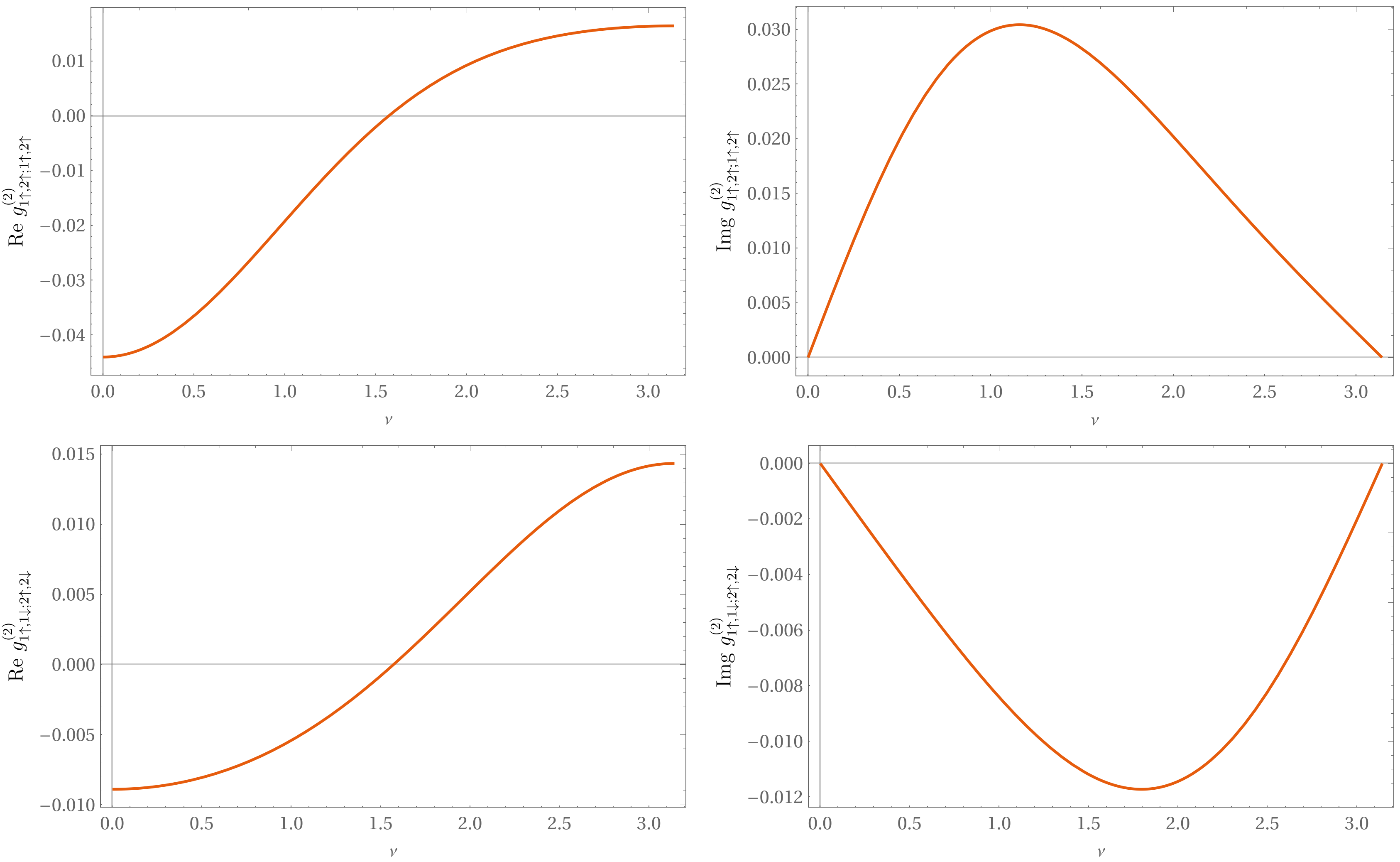
and can also be evaluated exactly. The full list of four-point correlation functions is given in Appendix F. In Figure 5 we show a few cases of how the four-point correlation functions depend upon the statistics parameter ν\nu.

Refer to caption
Figure 5: Plots showing dependence of four-point correlation functions on the statistical parameter(κ=1,U=4,V=1,J=0.25,μ=0.5,β=1\kappa=1,U=4,V=1,J=0.25,\mu=0.5,\beta=1). The real part and the imaginary part are separately plotted.

6 Quasi-momentum Distribution

The distribution of anyons in the quasi-momentum space is given by the Fourier transform of the correlation function

⟨nk,s⟩=∑j,j′ei​k​(j−j′)​gj,s;j′,s(1)\displaystyle\begin{aligned} \braket{n_{k,s}}=\sum_{j,j^{\prime}}e^{ik\left(j-j^{\prime}\right)}g^{(1)}_{j,s;j^{\prime},s}\end{aligned} (42)

where ⟨nk​s⟩\braket{n_{ks}} denotes the quasi-momentum distribution of spin-ss particles. Since the exact expressions for the correlation functions are known, it is straightforward to calculate the quasi-momentum distribution function. Note that since g(1)j↑;j′↑=g(1)j↓;j′↓g^{(1)}_{j\uparrow;j^{\prime}\uparrow}=g^{(1)}_{j\downarrow;j^{\prime}\downarrow}, the quasi-momentum distribution is same for spin-up and spin-down particles. In Figure 6, we plot the quasi-momentum distribution for various values of the statistics parameter.

Refer to caption
Figure 6: Quasi-momentum distribution is plotted against the momentum for different values of the statistical parameter (κ=1,U=4,V=1,J=0.25,μ=10,β=1\kappa=1,U=4,V=1,J=0.25,\mu=10,\beta=1).

7 Summary and Outlook

The entanglement of indistinguishable particles poses subtle challenges not present in the case of distinguishable particles. Ideas based on information theory come in handy to define a consistent scheme for defining standard tools like partial trace and reduced density matrix, and correspondingly measures like von Neumann entropy, even for indistinguishable particles.

When phrased in the language of second quantization, these ideas can further be extended beyond bosons and fermions – the context in which they were developed – to anyons, particles whose statistics is defined by a continuous parameter which allows one to interpolate between the bosonic and fermionic limits.

In this paper,built on an earlier paper [4] where anyonic statistics were realised as a consequence of the topology of the underlying space, the foregoing points were explored and reinforced in detail in the concrete case of the one-dimensional two-site anyonic Hubbard model. As a spin-off, some miscellaneous results concerning the one-particle density matrix, the pair correlation functions of anyons, their quasi-momentum distribution functions are derived with special emphasis on their dependence on the statistics parameter.

Whether the entanglement of anyons discussed in this paper is protected [24] [25] [26] is an open question, and requires coupling the anyonic Hubbard model to an environment. We hope to discuss this issue elsewhere.

Although in this paper anyonic statistics are introduced by hand into the definition of the Hubbard model, it is possible to relate the anyonic Hubbard model with the usual bosonic or fermionic Hubbard models through a Jordan-Wigner transformation [27]. The continuum limit of this model, in turn, is related to the Tomonaga-Luttinger liquid with a charge-vortex composite playing the role of an anyon [28]. It is also well-known that the Tomonaga-Luttinger liquid is related to the Calogero-Sutherland model which in itself is an effective theory of the fractional quantum Hall system in the lowest Landau level [29]. Clearly, there is a commonality in the anyonic properties of all these models. It is also of interest to study non-abelian generalisations of these results. A related issue worth exploring concerns entanglement in systems of indistinguishable particles satisfying exclusion statistics [30]. We hope to examine some of these issues in the near future.

Appendix A Basis Transformation

Consider a projective measurement on to the one-particle subspace ℬM(1)\mathcal{B}^{(1)}_{M} where the one-particle basis states are localized in MM. Then, by definition, the reduced density matrix is

ρM(N−1)​(Φ)=1𝒩M​∑k∈ℬM(1)ak​|Φ⟩​⟨Φ|​ak†\displaystyle\rho^{(N-1)}_{M}\left(\Phi\right)=\frac{1}{\mathcal{N}_{M}}\sum_{k\in\mathcal{B}^{(1)}_{M}}a_{k}\ket{\Phi}\bra{\Phi}a^{\dagger}_{k} (43)

where 𝒩M=⟨Φ|∑k∈ℬM(1)ak†​ak|Φ⟩\mathcal{N}_{M}=\braket{\Phi|\sum_{k\in\mathcal{B}^{(1)}_{M}}a^{\dagger}_{k}a_{k}|\Phi}. Consider a unitary transformation UU in the one-particle subspace ℬM(1)\mathcal{B}^{(1)}_{M} and the basis transformation

ak†=∑k~Uk​k~​bk~†,|k⟩∈ℬM(1)\displaystyle a^{\dagger}_{k}=\sum_{\tilde{k}}U_{k\tilde{k}}b^{\dagger}_{\tilde{k}},\quad\ket{k}\in\mathcal{B}^{(1)}_{M} (44)

Corresponding to the one-particle basis states |k⟩∉ℬM(1)\ket{k}\notin\mathcal{B}^{(1)}_{M}, we may choose ak†=bk~†a^{\dagger}_{k}=b^{\dagger}_{\tilde{k}}. However, these states do not appear in the expression for partial trace onto ℬM(1)\mathcal{B}^{(1)}_{M}.

We have

∑k∈ℬM(1)ak​|Φ⟩​⟨Φ|​ak†=∑k,i,j∈ℬM(1)Uk,i∗​Uk,j​bi​|Φ⟩​⟨Φ|​bj†=∑j∈ℬM(1)bj​|Φ⟩​⟨Φ|​bj†\displaystyle\begin{aligned} \sum_{k\in\mathcal{B}^{(1)}_{M}}a_{k}\ket{\Phi}\bra{\Phi}a^{\dagger}_{k}&=\sum_{k,i,j\in\mathcal{B}^{(1)}_{M}}U_{k,i}^{*}U_{k,j}b_{i}\ket{\Phi}\bra{\Phi}b_{j}^{\dagger}\\ &=\sum_{j\in\mathcal{B}^{(1)}_{M}}b_{j}\ket{\Phi}\bra{\Phi}b_{j}^{\dagger}\end{aligned} (45)

and

𝒩M=⟨Φ|∑k∈ℬM(1)ak†​ak|Φ⟩=⟨Φ|∑k,i,j∈ℬM(1)Uk,i∗​Uk,j​bi†​bj|Φ⟩=⟨Φ|∑j∈ℬM(1)bj†​bj|Φ⟩\displaystyle\begin{aligned} \mathcal{N}_{M}=\braket{\Phi|\sum_{k\in\mathcal{B}^{(1)}_{M}}a^{\dagger}_{k}a_{k}|\Phi}=\braket{\Phi|\sum_{k,i,j\in\mathcal{B}^{(1)}_{M}}U_{k,i}^{*}U_{k,j}b_{i}^{\dagger}b_{j}|\Phi}=\braket{\Phi|\sum_{j\in\mathcal{B}^{(1)}_{M}}b_{j}^{\dagger}b_{j}|\Phi}\end{aligned} (46)

Therefore, the reduced density matrix is given by

ρM(N−1)​(Φ)=1𝒩M​∑k∈ℬM(1)bk​|Φ⟩​⟨Φ|​bk†\displaystyle\rho^{(N-1)}_{M}\left(\Phi\right)=\frac{1}{\mathcal{N}_{M}}\sum_{k\in\mathcal{B}^{(1)}_{M}}b_{k}\ket{\Phi}\bra{\Phi}b^{\dagger}_{k} (47)

where 𝒩M=⟨Φ|∑k∈ℬM(1)bk†​bk|Φ⟩\mathcal{N}_{M}=\braket{\Phi|\sum_{k\in\mathcal{B}^{(1)}_{M}}b^{\dagger}_{k}b_{k}|\Phi}. This shows the definition of the reduced density matrix is independent of the choice of the basis of the one-particle subspace onto which the projective measurement is made.

Appendix B Eigenvalues and Eigenvectors of the Hamiltonian

The eigenvalues of the Hamiltonian are listed below.

ε0,1=0,ε1,1=ε1,3=−κ−με1,2=ε1,4=κ−με2,1=ε2,3=ε2,6=2​(−J​cos⁡(ν)−μ+V)ε2,2=U−2​με2,4=12​(−4​μ+Υ+v1)ε2,5=12​(−4​μ−Υ+v1)ε3,1=ε3,3=−κ−2​J​cos⁡(ν)−3​μ+U+4​Vε3,2=ε3,4=κ−2​J​cos⁡(ν)−3​μ+U+4​Vε4,1=2​(−2​J​cos⁡(ν)−2​μ+U+4​V)\displaystyle\begin{aligned} \varepsilon_{0,1}&=0,\\ \varepsilon_{1,1}&=\varepsilon_{1,3}=-\kappa-\mu\\ \varepsilon_{1,2}&=\varepsilon_{1,4}=\kappa-\mu\\ \varepsilon_{2,1}&=\varepsilon_{2,3}=\varepsilon_{2,6}=2(-J\cos(\nu)-\mu+V)\\ \varepsilon_{2,2}&=U-2\mu\\ \varepsilon_{2,4}&=\frac{1}{2}\left(-4\mu+\Upsilon+v_{1}\right)\\ \varepsilon_{2,5}&=\frac{1}{2}\left(-4\mu-\Upsilon+v_{1}\right)\\ \varepsilon_{3,1}&=\varepsilon_{3,3}=-\kappa-2J\cos(\nu)-3\mu+U+4V\\ \varepsilon_{3,2}&=\varepsilon_{3,4}=\kappa-2J\cos(\nu)-3\mu+U+4V\\ \varepsilon_{4,1}&=2(-2J\cos(\nu)-2\mu+U+4V)\end{aligned} (48)

where v1=2​J​cos⁡(ν)+U+2​Vv_{1}=2J\cos(\nu)+U+2V, v2=−2​J​cos⁡(ν)+U−2​Vv_{2}=-2J\cos(\nu)+U-2V and Υ=(16​κ2+v22)\Upsilon=\sqrt{\left(16\kappa^{2}+v_{2}^{2}\right)}. εj,k\varepsilon_{j,k} denotes the kt​hk^{th} eigenvalue of the j−j-particle Hamiltonian. The corresponding eigenvectors are

|ϕ0,1⟩=|0⟩|ϕ1,1⟩=|1↑⟩+|2↑⟩|ϕ1,2⟩=−|1↑⟩+|2↑⟩|ϕ1,3⟩=|1↓⟩+|2↓⟩|ϕ1,4⟩=−|1↓⟩+|2↓⟩|ϕ2,1⟩=|1↑,2↑⟩|ϕ2,2⟩=−e−i​ν​|1↑,1↓⟩+|2↑,2↓⟩|ϕ2,3⟩=|1↑,2↓⟩+|1↓,2↑⟩|ϕ2,4⟩=4​κ​e−i​νΥ−v2​|1↑,1↓⟩+4​κΥ−v2​|2↑,2↓⟩−|1↑,2↓⟩+|1↓,2↑⟩|ϕ2,5⟩=−4​κ​e−i​νΥ+v2​|1↑,1↓⟩−4​κΥ+v2​|2↑,2↓⟩−|1↑,2↓⟩+|1↓,2↑⟩|ϕ2,6⟩=|1↓,2↓⟩|ϕ3,1⟩=−e−i​ν​|1↑,1↓,2↑⟩+|1↑,2↑,2↓⟩|ϕ3,2⟩=e−i​ν​|1↑,1↓,2↑⟩+|1↑,2↑,2↓⟩|ϕ3,3⟩=−e−i​ν​|1↑,1↓,2↓⟩+|1↓,2↑,2↓⟩|ϕ3,4⟩=e−i​ν​|1↑,1↓,2↓⟩+|1↓,2↑,2↓⟩|ϕ4,1⟩=|1↑,1↓,2↑,2↓⟩\displaystyle\begin{aligned} \ket{\phi_{0,1}}&=\ket{0}\\ \ket{\phi_{1,1}}&=\ket{1\uparrow}+\ket{2\uparrow}\\ \ket{\phi_{1,2}}&=-\ket{1\uparrow}+\ket{2\uparrow}\\ \ket{\phi_{1,3}}&=\ket{1\downarrow}+\ket{2\downarrow}\\ \ket{\phi_{1,4}}&=-\ket{1\downarrow}+\ket{2\downarrow}\\ \ket{\phi_{2,1}}&=\ket{1\uparrow,2\uparrow}\\ \ket{\phi_{2,2}}&=-e^{-i\nu}\ket{1\uparrow,1\downarrow}+\ket{2\uparrow,2\downarrow}\\ \ket{\phi_{2,3}}&=\ket{1\uparrow,2\downarrow}+\ket{1\downarrow,2\uparrow}\\ \ket{\phi_{2,4}}&=\frac{4\kappa e^{-i\nu}}{\Upsilon-v_{2}}\ket{1\uparrow,1\downarrow}+\frac{4\kappa}{\Upsilon-v_{2}}\ket{2\uparrow,2\downarrow}-\ket{1\uparrow,2\downarrow}+\ket{1\downarrow,2\uparrow}\\ \ket{\phi_{2,5}}&=-\frac{4\kappa e^{-i\nu}}{\Upsilon+v_{2}}\ket{1\uparrow,1\downarrow}-\frac{4\kappa}{\Upsilon+v_{2}}\ket{2\uparrow,2\downarrow}-\ket{1\uparrow,2\downarrow}+\ket{1\downarrow,2\uparrow}\\ \ket{\phi_{2,6}}&=\ket{1\downarrow,2\downarrow}\\ \ket{\phi_{3,1}}&=-e^{-i\nu}\ket{1\uparrow,1\downarrow,2\uparrow}+\ket{1\uparrow,2\uparrow,2\downarrow}\\ \ket{\phi_{3,2}}&=e^{-i\nu}\ket{1\uparrow,1\downarrow,2\uparrow}+\ket{1\uparrow,2\uparrow,2\downarrow}\\ \ket{\phi_{3,3}}&=-e^{-i\nu\ }\ket{1\uparrow,1\downarrow,2\downarrow}+\ket{1\downarrow,2\uparrow,2\downarrow}\\ \ket{\phi_{3,4}}&=e^{-i\nu}\ket{1\uparrow,1\downarrow,2\downarrow}+\ket{1\downarrow,2\uparrow,2\downarrow}\\ \ket{\phi_{4,1}}&=\ket{1\uparrow,1\downarrow,2\uparrow,2\downarrow}\\ \end{aligned} (49)

Appendix C Reduced Density Matrices

Let ℬ1={|1↑⟩,|1↓⟩}\mathcal{B}_{1}=\{\ket{1\uparrow},\ket{1\downarrow}\} and ℬ2={|2↑⟩,|2↓⟩}\mathcal{B}_{2}=\{\ket{2\uparrow},\ket{2\downarrow}\} be the single-particle local bases at sites 1 and 2 respectively, and let the non-local basis be ℬ12={|1↑⟩,|1↓⟩,|2↑⟩,|2↓⟩}\mathcal{B}_{12}=\{\ket{1\uparrow},\ket{1\downarrow},\ket{2\uparrow},\ket{2\downarrow}\}. These will be used to perform the partial traces.

The reduced density matrices after performing a partial trace onto the one-particle subspace ℬ1={|1↑⟩,|1↓⟩}\mathcal{B}_{1}=\{\ket{1\uparrow},\ket{1\downarrow}\} are

ρ1(1)​(ϕ2,1)=|2↑⟩​⟨2↑|ρ1(1)​(ϕ2,2)=12​(|1↑⟩​⟨1↑|+|1↓⟩​⟨1↓|)ρ1(1)​(ϕ2,3)=12​(|2↑⟩​⟨2↑|+|2↓⟩​⟨2↓|)ρ1(1)​(ϕ2,4)=Υ+v24​Υ​(|1↑⟩​⟨1↑|+|1↓⟩​⟨1↓|)−κ​e−i​νΥ​(|1↑⟩​⟨2↑|+|1↓⟩​⟨2↓|)−κ​ei​νΥ​(|2↑⟩​⟨1↑|+|2↓⟩​⟨1↓|)+Υ−v24​Υ​(|2↑⟩​⟨2↑|+|2↓⟩​⟨2↓|)ρ1(1)​(ϕ2,5)=Υ−v24​Υ​(|1↑⟩​⟨1↑|+|1↓⟩​⟨1↓|)+κ​e−i​νΥ​(|1↑⟩​⟨2↑|+|1↓⟩​⟨2↓|)+κ​ei​νΥ​(|2↑⟩​⟨1↑|+|2↓⟩​⟨1↓|)+Υ+v24​Υ​(|2↑⟩​⟨2↑|+|2↓⟩​⟨2↓|)ρ1(1)​(ϕ2,6)=|2↓⟩​⟨2↓|\displaystyle\begin{aligned} \rho^{(1)}_{1}\left(\phi_{2,1}\right)&=\ket{2\uparrow}\bra{2\uparrow}\\ \rho^{(1)}_{1}\left(\phi_{2,2}\right)&=\frac{1}{2}\left(\ket{1\uparrow}\bra{1\uparrow}+\ket{1\downarrow}\bra{1\downarrow}\right)\\ \rho^{(1)}_{1}\left(\phi_{2,3}\right)&=\frac{1}{2}\left(\ket{2\uparrow}\bra{2\uparrow}+\ket{2\downarrow}\bra{2\downarrow}\right)\\ \rho^{(1)}_{1}\left(\phi_{2,4}\right)&=\frac{\Upsilon+v_{2}}{4\Upsilon}\left(\ket{1\uparrow}\bra{1\uparrow}+\ket{1\downarrow}\bra{1\downarrow}\right)-\frac{\kappa e^{-i\nu}}{\Upsilon}\left(\ket{1\uparrow}\bra{2\uparrow}+\ket{1\downarrow}\bra{2\downarrow}\right)\\ &\quad-\frac{\kappa e^{i\nu}}{\Upsilon}\left(\ket{2\uparrow}\bra{1\uparrow}+\ket{2\downarrow}\bra{1\downarrow}\right)+\frac{\Upsilon-v_{2}}{4\Upsilon}\left(\ket{2\uparrow}\bra{2\uparrow}+\ket{2\downarrow}\bra{2\downarrow}\right)\\ \rho^{(1)}_{1}\left(\phi_{2,5}\right)&=\frac{\Upsilon-v_{2}}{4\Upsilon}\left(\ket{1\uparrow}\bra{1\uparrow}+\ket{1\downarrow}\bra{1\downarrow}\right)+\frac{\kappa e^{-i\nu}}{\Upsilon}\left(\ket{1\uparrow}\bra{2\uparrow}+\ket{1\downarrow}\bra{2\downarrow}\right)\\ &\quad+\frac{\kappa e^{i\nu}}{\Upsilon}\left(\ket{2\uparrow}\bra{1\uparrow}+\ket{2\downarrow}\bra{1\downarrow}\right)+\frac{\Upsilon+v_{2}}{4\Upsilon}\left(\ket{2\uparrow}\bra{2\uparrow}+\ket{2\downarrow}\bra{2\downarrow}\right)\\ \rho^{(1)}_{1}\left(\phi_{2,6}\right)&=\ket{2\downarrow}\bra{2\downarrow}\\ \end{aligned} (50)

where v1=2​J​cos⁡(ν)+U+2​Vv_{1}=2J\cos(\nu)+U+2V, v2=−2​J​cos⁡(ν)+U−2​Vv_{2}=-2J\cos(\nu)+U-2V and Υ=(16​κ2+v22)\Upsilon=\sqrt{\left(16\kappa^{2}+v_{2}^{2}\right)}. The reduced density matrices after performing a partial trace onto the one-particle subspace ℬ2={|2↑⟩,|2↓⟩}\mathcal{B}_{2}=\{\ket{2\uparrow},\ket{2\downarrow}\} are

ρ2(1)​(ϕ2,1)=|1↑⟩​⟨1↑|ρ2(1)​(ϕ2,2)=12​(|2↑⟩​⟨2↑|+|2↓⟩​⟨2↓|)ρ2(1)​(ϕ2,3)=12​(|1↑⟩​⟨1↑|+|1↓⟩​⟨1↓|)ρ2(1)​(ϕ2,4)=Υ−v24​Υ​(|1↑⟩​⟨1↑|+|1↓⟩​⟨1↓|)−κ​e−i​νΥ​(|1↑⟩​⟨2↑|+|1↓⟩​⟨2↓|)−κ​ei​νΥ​(|2↑⟩​⟨1↑|+|2↓⟩​⟨1↓|)+Υ+v24​Υ​(|2↑⟩​⟨2↑|+|2↓⟩​⟨2↓|)ρ2(1)​(ϕ2,5)=Υ+v24​Υ​(|1↑⟩​⟨1↑|+|1↓⟩​⟨1↓|)+κ​e−i​νΥ​(|1↑⟩​⟨2↑|+|1↓⟩​⟨2↓|)+κ​ei​νΥ​(|2↑⟩​⟨1↑|+|2↓⟩​⟨1↓|)+Υ−v24​Υ​(|2↑⟩​⟨2↑|+|2↓⟩​⟨2↓|)ρ2(1)​(ϕ2,6)=|1↓⟩​⟨1↓|\displaystyle\begin{aligned} \rho^{(1)}_{2}\left(\phi_{2,1}\right)&=\ket{1\uparrow}\bra{1\uparrow}\\ \rho^{(1)}_{2}\left(\phi_{2,2}\right)&=\frac{1}{2}\left(\ket{2\uparrow}\bra{2\uparrow}+\ket{2\downarrow}\bra{2\downarrow}\right)\\ \rho^{(1)}_{2}\left(\phi_{2,3}\right)&=\frac{1}{2}\left(\ket{1\uparrow}\bra{1\uparrow}+\ket{1\downarrow}\bra{1\downarrow}\right)\\ \rho^{(1)}_{2}\left(\phi_{2,4}\right)&=\frac{\Upsilon-v_{2}}{4\Upsilon}\left(\ket{1\uparrow}\bra{1\uparrow}+\ket{1\downarrow}\bra{1\downarrow}\right)-\frac{\kappa e^{-i\nu}}{\Upsilon}\left(\ket{1\uparrow}\bra{2\uparrow}+\ket{1\downarrow}\bra{2\downarrow}\right)\\ &\quad-\frac{\kappa e^{i\nu}}{\Upsilon}\left(\ket{2\uparrow}\bra{1\uparrow}+\ket{2\downarrow}\bra{1\downarrow}\right)+\frac{\Upsilon+v_{2}}{4\Upsilon}\left(\ket{2\uparrow}\bra{2\uparrow}+\ket{2\downarrow}\bra{2\downarrow}\right)\\ \rho^{(1)}_{2}\left(\phi_{2,5}\right)&=\frac{\Upsilon+v_{2}}{4\Upsilon}\left(\ket{1\uparrow}\bra{1\uparrow}+\ket{1\downarrow}\bra{1\downarrow}\right)+\frac{\kappa e^{-i\nu}}{\Upsilon}\left(\ket{1\uparrow}\bra{2\uparrow}+\ket{1\downarrow}\bra{2\downarrow}\right)\\ &\quad+\frac{\kappa e^{i\nu}}{\Upsilon}\left(\ket{2\uparrow}\bra{1\uparrow}+\ket{2\downarrow}\bra{1\downarrow}\right)+\frac{\Upsilon-v_{2}}{4\Upsilon}\left(\ket{2\uparrow}\bra{2\uparrow}+\ket{2\downarrow}\bra{2\downarrow}\right)\\ \rho^{(1)}_{2}\left(\phi_{2,6}\right)&=\ket{1\downarrow}\bra{1\downarrow}\\ \end{aligned} (51)

Similarly, the reduced density matrices after performing a partial trace onto the one-particle subspace ℬ12={|1↑⟩,|1↓⟩,|2↑⟩,|2↓⟩}\mathcal{B}_{12}=\{\ket{1\uparrow},\ket{1\downarrow},\ket{2\uparrow},\ket{2\downarrow}\} are

ρ12(1)​(ϕ2,1)=12​(|1↑⟩​⟨1↑|+|2↑⟩​⟨2↑|)ρ12(1)​(ϕ2,2)=14​(|1↑⟩​⟨1↑|+|2↑⟩​⟨2↑|+|1↓⟩​⟨1↓|+|2↓⟩​⟨2↓|)ρ12(1)​(ϕ2,3)=14​(|1↑⟩​⟨1↑|+|2↑⟩​⟨2↑|+|1↓⟩​⟨1↓|+|2↓⟩​⟨2↓|)ρ12(1)​(ϕ2,4)=14​(|1↑⟩​⟨1↑|+|1↓⟩​⟨1↓|)−κ​e−i​νΥ​(|1↑⟩​⟨2↑|+|1↓⟩​⟨2↓|)−κ​ei​νΥ​(|2↑⟩​⟨1↑|+|2↓⟩​⟨1↓|)+14​(|2↑⟩​⟨2↑|+|2↓⟩​⟨2↓|)ρ12(1)​(ϕ2,5)=14​(|1↑⟩​⟨1↑|+|1↓⟩​⟨1↓|)+κ​e−i​νΥ​(|1↑⟩​⟨2↑|+|1↓⟩​⟨2↓|)+κ​ei​νΥ​(|2↑⟩​⟨1↑|+|2↓⟩​⟨1↓|)+14​(|2↑⟩​⟨2↑|+|2↓⟩​⟨2↓|)ρ12(1)​(ϕ2,6)=12​(|1↓⟩​⟨1↓|+|2↓⟩​⟨2↓|)\displaystyle\begin{aligned} \rho^{(1)}_{12}\left(\phi_{2,1}\right)&=\frac{1}{2}\left(\ket{1\uparrow}\bra{1\uparrow}+\ket{2\uparrow}\bra{2\uparrow}\right)\\ \rho^{(1)}_{12}\left(\phi_{2,2}\right)&=\frac{1}{4}\left(\ket{1\uparrow}\bra{1\uparrow}+\ket{2\uparrow}\bra{2\uparrow}+\ket{1\downarrow}\bra{1\downarrow}+\ket{2\downarrow}\bra{2\downarrow}\right)\\ \rho^{(1)}_{12}\left(\phi_{2,3}\right)&=\frac{1}{4}\left(\ket{1\uparrow}\bra{1\uparrow}+\ket{2\uparrow}\bra{2\uparrow}+\ket{1\downarrow}\bra{1\downarrow}+\ket{2\downarrow}\bra{2\downarrow}\right)\\ \rho^{(1)}_{12}\left(\phi_{2,4}\right)&=\frac{1}{4}\left(\ket{1\uparrow}\bra{1\uparrow}+\ket{1\downarrow}\bra{1\downarrow}\right)-\frac{\kappa e^{-i\nu}}{\Upsilon}\left(\ket{1\uparrow}\bra{2\uparrow}+\ket{1\downarrow}\bra{2\downarrow}\right)\\ &\quad-\frac{\kappa e^{i\nu}}{\Upsilon}\left(\ket{2\uparrow}\bra{1\uparrow}+\ket{2\downarrow}\bra{1\downarrow}\right)+\frac{1}{4}\left(\ket{2\uparrow}\bra{2\uparrow}+\ket{2\downarrow}\bra{2\downarrow}\right)\\ \rho^{(1)}_{12}\left(\phi_{2,5}\right)&=\frac{1}{4}\left(\ket{1\uparrow}\bra{1\uparrow}+\ket{1\downarrow}\bra{1\downarrow}\right)+\frac{\kappa e^{-i\nu}}{\Upsilon}\left(\ket{1\uparrow}\bra{2\uparrow}+\ket{1\downarrow}\bra{2\downarrow}\right)\\ &\quad+\frac{\kappa e^{i\nu}}{\Upsilon}\left(\ket{2\uparrow}\bra{1\uparrow}+\ket{2\downarrow}\bra{1\downarrow}\right)+\frac{1}{4}\left(\ket{2\uparrow}\bra{2\uparrow}+\ket{2\downarrow}\bra{2\downarrow}\right)\\ \rho^{(1)}_{12}\left(\phi_{2,6}\right)&=\frac{1}{2}\left(\ket{1\downarrow}\bra{1\downarrow}+\ket{2\downarrow}\bra{2\downarrow}\right)\end{aligned} (52)

Appendix D Time Evolution in the Presence of an External Field

From the block structure of the Hamiltonian, it is clear that in the presence of an external field the state |Φi(2)⟩=|1↑,1↓⟩\ket{\Phi_{i}^{(2)}}=\ket{1\uparrow,1\downarrow} is evolved by a time evolution operator W~​(t)\tilde{W}(t) which is the solution of the equation

i​d​W~​(t)d​t=H2,0​(t)​W~​(t)\displaystyle\begin{aligned} i\dfrac{d\tilde{W}(t)}{dt}=H_{2,0}(t)\tilde{W}(t)\end{aligned} (53)

where

H2,0​(t)=(U−2​μ0−κ​e−i⁡(ν−Ω​t)κ​e−i⁡(ν−Ω​t)0U−2​μ−κ​e−i​Ω​tκ​e−i​Ω​t−κ​ei⁡(ν−Ω​t)−κ​ei​Ω​t2​(V−μ)−2​J​cos⁡(ν)κ​ei⁡(ν−Ω​t)κ​ei​Ω​t−2​J​cos⁡(ν)2​(V−μ))\displaystyle\begin{aligned} H_{2,0}(t)&=\left(\begin{array}[]{cccc}U-2\mu&0&-\kappa e^{-i(\nu-\Omega t)}&\kappa e^{-i(\nu-\Omega t)}\\ 0&U-2\mu&-\kappa e^{-i\Omega t}&\kappa e^{-i\Omega t}\\ -\kappa e^{i(\nu-\Omega t)}&-\kappa e^{i\Omega t}&2(V-\mu)&-2J\cos(\nu)\\ \kappa e^{i(\nu-\Omega t)}&\kappa e^{i\Omega t}&-2J\cos(\nu)&2(V-\mu)\\ \end{array}\right)\end{aligned} (54)

Here the matrix representation of the Hamiltonian is given in the basis

{|1↑,1↓⟩,|2↑,2↓⟩,|1↑,2↓⟩,|1↓,2↑⟩}.\{\ket{1\uparrow,1\downarrow},\ket{2\uparrow,2\downarrow},\ket{1\uparrow,2\downarrow},\ket{1\downarrow,2\uparrow}\}.

The time evolution operator W~​(t)\tilde{W}(t) can be found as discussed in section 3.2 and is given by W~​(t)=W1​e−i​H~2,0​t\tilde{W}(t)=W_{1}e^{-i\tilde{H}_{2,0}t} where W1=diag​{e−i​Ω​t,ei​Ω​t,1,1}W_{1}=\text{diag}\{e^{-i\Omega t},e^{i\Omega t},1,1\} and

H~2,0=(U−2​μ+Ω0−κ​e−i​νκ​e−i​ν0U−2​μ−Ω−κκ−κ​ei​ν−κ2​(V−μ)−2​J​cos⁡(ν)κ​ei​νκ−2​J​cos⁡(ν)2​(V−μ))\displaystyle\begin{aligned} \tilde{H}_{2,0}=\left(\begin{array}[]{cccc}U-2\mu+\Omega&0&-\kappa e^{-i\nu}&\kappa e^{-i\nu}\\ 0&U-2\mu-\Omega&-\kappa&\kappa\\ -\kappa e^{i\nu}&-\kappa&2(V-\mu)&-2J\cos(\nu)\\ \kappa e^{i\nu}&\kappa&-2J\cos(\nu)&2(V-\mu)\\ \end{array}\right)\end{aligned} (55)

Even though we can obtain W~​(t)\tilde{W}(t) exactly, we will not discuss it here as the expressions are long and cumbersome. However we will give the following argument to establish certain relations among the matrix elements of W~​(t)\tilde{W}(t).

In the presence of the external field, the state |Φi(2)⟩\ket{\Phi_{i}^{(2)}} evolves into a state of the form

|Φo(2)⟩=W~​(t)​|Φi(2)⟩=W~11​(t)​|1↑,1↓⟩+W~12​(t)​|2↑,2↓⟩+W~13​(t)​|1↑,2↓⟩+W~14​(t)​|1↓,2↑⟩\displaystyle\begin{aligned} \ket{\Phi_{o}^{(2)}}=\tilde{W}(t)\ket{\Phi_{i}^{(2)}}=\tilde{W}_{11}(t)\ket{1\uparrow,1\downarrow}+\tilde{W}_{12}(t)\ket{2\uparrow,2\downarrow}+\tilde{W}_{13}(t)\ket{1\uparrow,2\downarrow}+\tilde{W}_{14}(t)\ket{1\downarrow,2\uparrow}\end{aligned} (56)

where W~m,n​(t)\tilde{W}_{m,n}(t) are matrix elements of W~​(t)\tilde{W}(t). Since W~​(t)\tilde{W}(t) is a unitary operator, it is clear that |W~11​(t)|2+|W~12​(t)|2+|W~13​(t)|2+|W~14​(t)|2=1|\tilde{W}_{11}(t)|^{2}+|\tilde{W}_{12}(t)|^{2}+|\tilde{W}_{13}(t)|^{2}+|\tilde{W}_{14}(t)|^{2}=1.

Note that the Hamiltonian H~2,0\tilde{H}_{2,0} is invariant under the unitary similarity transformation

P​H~2,0​P†=H~2,0P\tilde{H}_{2,0}P^{\dagger}=\tilde{H}_{2,0}

where

P=(10000100000−100−10)\displaystyle\begin{aligned} P=\left(\begin{array}[]{cccc}1&0&0&0\\ 0&1&0&0\\ 0&0&0&-1\\ 0&0&-1&0\\ \end{array}\right)\end{aligned} (57)

This, in turn, also means that W~​(t)\tilde{W}(t) is invariant under the unitary similarity transformation by the matrix PP. Therefore we can conclude that W~14​(t)=−W~13​(t)\tilde{W}_{14}(t)=-\tilde{W}_{13}(t) resulting in the output state

|Φo(2)⟩=W~11​(t)​|1↑,1↓⟩+W~12​(t)​|2↑,2↓⟩+W~13​(t)​(|1↑,2↓⟩−|1↓,2↑⟩)\displaystyle\begin{aligned} \ket{\Phi_{o}^{(2)}}=\tilde{W}_{11}(t)\ket{1\uparrow,1\downarrow}+\tilde{W}_{12}(t)\ket{2\uparrow,2\downarrow}+\tilde{W}_{13}(t)\left(\ket{1\uparrow,2\downarrow}-\ket{1\downarrow,2\uparrow}\right)\end{aligned} (58)

Identifying c1​(t)=W~11​(t),c2​(t)=2​W~13​(t)c_{1}(t)=\tilde{W}_{11}(t),c_{2}(t)=\sqrt{2}\tilde{W}_{13}(t) and c3​(t)=W~12​(t)c_{3}(t)=\tilde{W}_{12}(t) we obtain the result in equation 39.

Appendix E Partition Function

The partition function is easily calculated and is given below.

Z=1+2​eβ⁡(κ+μ)+2​e−β⁡(κ−μ)+2​e−β⁡(−κ+U+4​V−2​J​cos⁡(ν)−3​μ)+2​e−β⁡(κ+U+4​V−2​J​cos⁡(ν)−3​μ)+e−2​β​(U+4​V−2​J​cos⁡(ν)−2​μ)+3​e−2​β​(V−J​cos⁡(ν)−μ)+e−β⁡(U−2​μ)+e−12​β​(−4​μ−16​κ2+v22+v1)+e−12​β​(−4​μ+16​κ2+v22+v1)\displaystyle\begin{aligned} Z&=1+2e^{\beta(\kappa+\mu)}+2e^{-\beta(\kappa-\mu)}+2e^{-\beta(-\kappa+U+4V-2J\cos(\nu)-3\mu)}+2e^{-\beta(\kappa+U+4V-2J\cos(\nu)-3\mu)}\\ &+e^{-2\beta(U+4V-2J\cos(\nu)-2\mu)}+3e^{-2\beta(V-J\cos(\nu)-\mu)}+e^{-\beta(U-2\mu)}+e^{-\frac{1}{2}\beta\left(-4\mu-\sqrt{16\kappa^{2}+v_{2}^{2}}+v_{1}\right)}\\ &+e^{-\frac{1}{2}\beta\left(-4\mu+\sqrt{16\kappa^{2}+v_{2}^{2}}+v_{1}\right)}\end{aligned} (59)

where v1=2​J​cos⁡(ν)+U+2​Vv_{1}=2J\cos(\nu)+U+2V, v2=−2​J​cos⁡(ν)+U−2​Vv_{2}=-2J\cos(\nu)+U-2V and Υ=(16​κ2+v22)\Upsilon=\sqrt{\left(16\kappa^{2}+v_{2}^{2}\right)}. Note that the partition function reduces to the fermionic case in the limit ν=0\nu=0 and to the (pseudo-)bosonic case in the limit ν=π\nu=\pi.

Appendix F Correlation Functions

The correlation functions can be calculated exactly since the exact solution of the two-site Anyonic Hubbard Model are known. The two-point correlation functions are

gi,s;i,s(1)=12​Z​(e−β​ε1,1+e−β​ε1,2+3​e−β​ε2,1+e−β​ε2,2CLOSEOPEN+e−β​ε2,4+e−β​ε2,5+3​e−β​ε3,1+3​e−β​ε3,2+2​e−β​ε4,1)gi,s;j,s(1)=12​Z​(−4​κ​e−β​ε2,4Υ+4​κ​e−β​ε2,5Υ+e−β​ε1,1−e−β​ε1,2+e−β​ε3,1−e−β​ε3,2),i≠jgi,s;j,s′(1)=0,s≠s′\displaystyle\begin{aligned} g^{(1)}_{i,s;i,s}=&\frac{1}{2Z}\bigg(e^{-\beta\varepsilon_{1,1}}+e^{-\beta\varepsilon_{1,2}}+3e^{-\beta\varepsilon_{2,1}}+e^{-\beta\varepsilon_{2,2}}\\ &+e^{-\beta\varepsilon_{2,4}}+e^{-\beta\varepsilon_{2,5}}+3e^{-\beta\varepsilon_{3,1}}+3e^{-\beta\varepsilon_{3,2}}+2e^{-\beta\varepsilon_{4,1}}\bigg)\\ g^{(1)}_{i,s;j,s}&=\frac{1}{2Z}\left(-\frac{4\kappa e^{-\beta\varepsilon_{2,4}}}{\Upsilon}+\frac{4\kappa e^{-\beta\varepsilon_{2,5}}}{\Upsilon}+e^{-\beta\varepsilon_{1,1}}-e^{-\beta\varepsilon_{1,2}}+e^{-\beta\varepsilon_{3,1}}-e^{-\beta\varepsilon_{3,2}}\right),\quad i\neq j\\ g^{(1)}_{i,s;j,s^{\prime}}&=0,\quad s\neq s^{\prime}\end{aligned} (60)

where εm,n\varepsilon_{m,n} is the nthn^{\text{th}} eigenvalue of m−m-particle Hamiltonian, i,j=1,2i,j=1,2 and s,s′=↑,↓s,s^{\prime}=\uparrow,\downarrow.

Similarly, the four-point correlation functions can be exactly calculated. The distinct cases of the four-point correlation functions are

g(2)1↑,2↑;1↑,2↑=e−i​ν​(−e−β​ε2,1−e−β​ε3,1−e−β​ε3,2−e−β​ε4,1)g(2)1↑,1↓;1↑,1↓=14​(−2​e−β​ε2,2−e−β​ε2,4−e−β​ε2,5−4​e−β​ε3,1−4​e−β​ε3,2−4​e−β​ε4,1CLOSEOPEN+v2​(e−β​ε2,5−e−β​ε2,4)Υ)g(2)1↑,1↓;2↑,2↓=14​ei​ν​(2​e−β​ε2,2−e−β​ε2,4−e−β​ε2,5+v2​(e−β​ε2,5−e−β​ε2,4)Υ)g(2)1↑,1↓;1↑,2↓=2​κ​e−β​ε2,4−2​κ​e−β​ε2,5−Υ​e−β​ε3,1+Υ​e−β​ε3,22​Υg(2)1↑,2↓;1↑,2↓=14​e−i​ν​(−2​e−β​ε2,1−4​e−β​ε3,1−4​e−β​ε3,2−4​e−β​ε4,1CLOSEOPEN+(v2−Υ)​e−β​ε2,4Υ−(Υ+v2)​e−β​ε2,5Υ)g(2)1↑,2↓;1↓,2↑=e−i​ν4​Υ​(−2​Υ​e−β​ε2,1+(Υ−v2)​e−β​ε2,4+(Υ+v2)​e−β​ε2,5)gj1,s1,j2,s2;j3,s3,j4,s4(2)=0​ if ​s1+s2≠s3+s4\displaystyle\begin{aligned} g^{(2)}_{1\uparrow,2\uparrow;1\uparrow,2\uparrow}=&e^{-i\nu}\left(-e^{-\beta\varepsilon_{2,1}}-e^{-\beta\varepsilon_{3,1}}-e^{-\beta\varepsilon_{3,2}}-e^{-\beta\varepsilon_{4,1}}\right)\\ g^{(2)}_{1\uparrow,1\downarrow;1\uparrow,1\downarrow}=&\frac{1}{4}\bigg(-2e^{-\beta\varepsilon_{2,2}}-e^{-\beta\varepsilon_{2,4}}-e^{-\beta\varepsilon_{2,5}}-4e^{-\beta\varepsilon_{3,1}}-4e^{-\beta\varepsilon_{3,2}}-4e^{-\beta\varepsilon_{4,1}}\\ &+\frac{v_{2}\left(e^{-\beta\varepsilon_{2,5}}-e^{-\beta\varepsilon_{2,4}}\right)}{\Upsilon}\bigg)\\ g^{(2)}_{1\uparrow,1\downarrow;2\uparrow,2\downarrow}=&\frac{1}{4}e^{i\nu}\left(2e^{-\beta\varepsilon_{2,2}}-e^{-\beta\varepsilon_{2,4}}-e^{-\beta\varepsilon_{2,5}}+\frac{v_{2}\left(e^{-\beta\varepsilon_{2,5}}-e^{-\beta\varepsilon_{2,4}}\right)}{\Upsilon}\right)\\ g^{(2)}_{1\uparrow,1\downarrow;1\uparrow,2\downarrow}=&\frac{2\kappa e^{-\beta\varepsilon_{2,4}}-2\kappa e^{-\beta\varepsilon_{2,5}}-\Upsilon e^{-\beta\varepsilon_{3,1}}+\Upsilon e^{-\beta\varepsilon_{3,2}}}{2\Upsilon}\\ g^{(2)}_{1\uparrow,2\downarrow;1\uparrow,2\downarrow}=&\frac{1}{4}e^{-i\nu}\bigg(-2e^{-\beta\varepsilon_{2,1}}-4e^{-\beta\varepsilon_{3,1}}-4e^{-\beta\varepsilon_{3,2}}-4e^{-\beta\varepsilon_{4,1}}\\ &+\frac{\left(v_{2}-\Upsilon\right)e^{-\beta\varepsilon_{2,4}}}{\Upsilon}-\frac{\left(\Upsilon+v_{2}\right)e^{-\beta\varepsilon_{2,5}}}{\Upsilon}\bigg)\\ g^{(2)}_{1\uparrow,2\downarrow;1\downarrow,2\uparrow}=&\frac{e^{-i\nu}}{4\Upsilon}\left(-2\Upsilon e^{-\beta\varepsilon_{2,1}}+\left(\Upsilon-v_{2}\right)e^{-\beta\varepsilon_{2,4}}+\left(\Upsilon+v_{2}\right)e^{-\beta\varepsilon_{2,5}}\right)\\ g^{(2)}_{j_{1},s_{1},j_{2},s_{2};j_{3},s_{3},j_{4},s_{4}}=&0\text{ if }s_{1}+s_{2}\neq s_{3}+s_{4}\end{aligned} (61)

We can obtain the other four-point correlation functions using the following relations

g(2)1↑,2↑;1↑,2↑=g(2)1↓,2↓;1↓,2↓g(2)1↑,1↓;1↑,1↓=g(2)2↑,2↓;2↑,2↓g(2)1↑,1↓;1↑,2↓=−g(2)1↑,1↓;1↓,2↑=e−i​νg(2)2↑,2↓;1↑,2↓=−e−i​νg(2)2↑,2↓;1↓,2↑=e−i​νg(2)1↑,2↓;1↑,1↓=g(2)1↑,2↓;2↑,2↓=−e−i​νg(2)1↓,2↑;1↑,1↓=−g(2)1↓,2↑;2↑,2↓\displaystyle\begin{aligned} g^{(2)}_{1\uparrow,2\uparrow;1\uparrow,2\uparrow}&=g^{(2)}_{1\downarrow,2\downarrow;1\downarrow,2\downarrow}\\ g^{(2)}_{1\uparrow,1\downarrow;1\uparrow,1\downarrow}&=g^{(2)}_{2\uparrow,2\downarrow;2\uparrow,2\downarrow}\\ g^{(2)}_{1\uparrow,1\downarrow;1\uparrow,2\downarrow}&=-g^{(2)}_{1\uparrow,1\downarrow;1\downarrow,2\uparrow}=e^{-i\nu}g^{(2)}_{2\uparrow,2\downarrow;1\uparrow,2\downarrow}=-e^{-i\nu}g^{(2)}_{2\uparrow,2\downarrow;1\downarrow,2\uparrow}\\ &=e^{-i\nu}g^{(2)}_{1\uparrow,2\downarrow;1\uparrow,1\downarrow}=g^{(2)}_{1\uparrow,2\downarrow;2\uparrow,2\downarrow}=-e^{-i\nu}g^{(2)}_{1\downarrow,2\uparrow;1\uparrow,1\downarrow}=-g^{(2)}_{1\downarrow,2\uparrow;2\uparrow,2\downarrow}\end{aligned} (62)

References

  • [1] Alexei Kitaev. Anyons in an exactly solved model and beyond. Annals of Physics, 321(1):2–111, 2006.
  • [2] John Preskill. Battling decoherence: The fault-tolerant quantum computer. Physics Today, 52(6):24–30, June 1999.
  • [3] Sankar Das Sarma, Michael Freedman, and Chetan Nayak. Topological quantum computation. Physics Today, 59(7):32–38, 2006.
  • [4] H. S. Mani, Ramadas N, and V. V. Sreedhar. Quantum entanglement in one-dimensional anyons. Physical Review A, 101(2):022314, February 2020.
  • [5] J. M. Leinaas and J. Myrheim. On the theory of identical particles. Il Nuovo Cimento B (1971-1996), 37(1):1–23, January 1977.
  • [6] Rosario Lo Franco and Giuseppe Compagno. Quantum entanglement of identical particles by standard information-theoretic notions. Scientific reports, 6:20603, 2016.
  • [7] Giuseppe Compagno, Alessia Castellini, and Rosario Lo Franco. Dealing with indistinguishable particles and their entanglement. Philosophical Transactions of the Royal Society A: Mathematical, Physical and Engineering Sciences, 376(2123):20170317, 2018.
  • [8] Thore Posske, Björn Trauzettel, and Michael Thorwart. Second quantization of Leinaas-Myrheim anyons in one dimension and their relation to the Lieb-Liniger model. Physical Review B, 96(19):195422, 2017.
  • [9] J. Hubbard and Brian Hilton Flowers. Electron correlations in narrow energy bands. Proceedings of the Royal Society of London. Series A. Mathematical and Physical Sciences, 276(1365):238–257, November 1963.
  • [10] Michael A. Nielsen and Isaac Chuang. Quantum Computation and Quantum Information. American Journal of Physics, 70(5):558, April 2002.
  • [11] AP Balachandran, TR Govindarajan, Amilcar R de Queiroz, and AF Reyes-Lega. Algebraic approach to entanglement and entropy. Physical Review A, 88(2):022301, 2013.
  • [12] GianCarlo Ghirardi and Luca Marinatto. Identical particles and entanglement. Optics and Spectroscopy, 99(3):386–390, 2005.
  • [13] John Schliemann, J Ignacio Cirac, Marek Kuś, Maciej Lewenstein, and Daniel Loss. Quantum correlations in two-fermion systems. Physical Review A, 64(2):022303, 2001.
  • [14] R Paškauskas and L You. Quantum correlations in two-boson wave functions. Physical Review A, 64(4):042310, 2001.
  • [15] Howard Mark Wiseman and John A Vaccaro. Entanglement of indistinguishable particles shared between two parties. Physical review letters, 91(9):097902, 2003.
  • [16] N Killoran, M Cramer, and Martin B Plenio. Extracting entanglement from identical particles. Physical review letters, 112(15):150501, 2014.
  • [17] Rosario Lo Franco and Giuseppe Compagno. Indistinguishability of elementary systems as a resource for quantum information processing. Physical review letters, 120(24):240403, 2018.
  • [18] Fabio Benatti, Roberto Floreanini, and Kelvin Titimbo. Entanglement of identical particles. Open Systems & Information Dynamics, 21(01n02):1440003, 2014.
  • [19] Kai Sun, Yan Wang, Zheng-Hao Liu, Xiao-Ye Xu, Jin-Shi Xu, Chuan-Feng Li, Guang-Can Guo, Alessia Castellini, Farzam Nosrati, Giuseppe Compagno, and Rosario Lo Franco. Experimental quantum entanglement and teleportation by tuning remote spatial indistinguishability of independent photons. Optics Letters, 45(23):6410–6413, December 2020.
  • [20] Kai Sun, Zheng-Hao Liu, Yan Wang, Ze-Yan Hao, Xiao-Ye Xu, Jin-Shi Xu, Chuan-Feng Li, Guang-Can Guo, Alessia Castellini, Ludovico Lami, Andreas Winter, Gerardo Adesso, Giuseppe Compagno, and Rosario Lo Franco. Experimental quantum phase discrimination enhanced by controllable indistinguishability-based coherence. arXiv:2103.14802 [quant-ph], March 2021.
  • [21] F. Benatti, R. Floreanini, F. Franchini, and U. Marzolino. Entanglement in indistinguishable particle systems. Physics Reports, 878:1–27, September 2020.
  • [22] Fabian H. L. Essler, Holger Frahm, Frank Göhmann, Andreas Klümper, and Vladimir E. Korepin. The One-Dimensional Hubbard Model. Cambridge University Press, February 2005.
  • [23] Shankar Balasubramanian and J. K. Freericks. Exact Time Evolution of the Asymmetric Hubbard Dimer. Journal of Superconductivity and Novel Magnetism, 30(1):97–102, January 2017.
  • [24] Matteo Piccolini, Farzam Nosrati, Giuseppe Compagno, Patrizia Livreri, Roberto Morandotti, and Rosario Lo Franco. Entanglement Robustness via Spatial Deformation of Identical Particle Wave Functions. Entropy, 23(6):708, June 2021.
  • [25] Farzam Nosrati, Alessia Castellini, Giuseppe Compagno, and Rosario Lo Franco. Robust entanglement preparation against noise by controlling spatial indistinguishability. npj Quantum Information, 6(1):1–7, May 2020.
  • [26] Farzam Nosrati, Alessia Castellini, Giuseppe Compagno, and Rosario Lo Franco. Dynamics of spatially indistinguishable particles and quantum entanglement protection. Physical Review A, 102(6):062429, December 2020.
  • [27] Tassilo Keilmann, Simon Lanzmich, Ian McCulloch, and Marco Roncaglia. Statistically induced phase transitions and anyons in 1D optical lattices. Nature Communications, 2(1):361, June 2011.
  • [28] Z. N. C. Ha. Exact Dynamical Correlation Functions of Calogero-Sutherland Model and One-Dimensional Fractional Statistics. Physical Review Letters, 73(12):1574–1577, September 1994.
  • [29] Stéphane Ouvry and Alexios P. Polychronakos. Mapping the Calogero model on the anyon model. Nuclear Physics B, 936:189–205, November 2018.
  • [30] F. D. M. Haldane. “Fractional statistics” in arbitrary dimensions: A generalization of the Pauli principle. Physical Review Letters, 67(8):937–940, August 1991.