Spatial Location Constraint Prototype Loss for Open Set Recognition
Abstract
One of the challenges in pattern recognition is open set recognition. Compared with closed set recognition, open set recognition needs to reduce not only the empirical risk, but also the open space risk, and the reduction of these two risks corresponds to classifying the known classes and identifying the unknown classes respectively. How to reduce the open space risk is the key of open set recognition. This paper explores the origin of the open space risk by analyzing the distribution of known and unknown classes features. On this basis, the spatial location constraint prototype loss function is proposed to reduce the two risks simultaneously. Extensive experiments on multiple benchmark datasets and many visualization results indicate that our methods is superior to most existing approaches. The code is released on https://github.com/Xiaziheng89/Spatial-Location-Constraint-Prototype-Loss-for-Open-Set-Recognition.
1 Introduction
With the development of deep learning technology, pattern recognition based on deep neural network has been greatly developed, such as image recognition and speech recognition face-recognition; speech-recognition. Although some deep learning methods have achieved great success, there are still many challenges and difficulties that need to be addressed in these applications. One of these challenges is that the test set may contain some classes that are not present in the training set. Unfortunately, the traditional deep neural network is incapable of detecting unknown classes. Therefore, open set recognition (OSR) was proposed to solve this kind of problem that the model needs to not only correctly classify known classes, but also identify unknown classes1-vs-set.
In contrast to OSR, the test set and the training set contain the same data categories in closed set recognition (CSR), and classifying known classes correctly corresponds to reducing the empirical risk. Therefore, OSR needs to reduce not only the empirical risk, but also the open space risk1-vs-set, which corresponds to identifying unknown classes effectively.
Due to the strong feature extraction ability, there is no doubt that deep neural network can do well in CSR. As shown in Fig.1(a), the LeNet++ trained with SoftMax can classify MNIST effectively. However, it can be seen from Fig.1(d) that there is obvious overlap between known and unknown classes features. The overlapping of these features in the feature space is the direct cause of the open space risk.
In order to reduce the two risks simultaneously, Yang et al. proposed the generalized convolutional prototype learning (GCPL) for robust classification and OSRGCPL; CPN. It can be seen from Fig.1(b) that the LeNet++ trained with GCPL can classify MNIST effectively. With regard to the open space risk, as shown in Fig.1(e), although much better than SoftMax, there are still three clusters of known features that overlap with unknown features. Similar to SoftMax, it will be seen from Section 3 that the way GCPL trains the network has disadvantages in reducing the open space risk.


As shown in Figs.1(d) and 1(e), we already know that the direct cause of the open space risk is that known and unknown classes features overlap in the feature space. In other words, if we can figure out why they overlap, then it’s possible to significantly reduce, or even eliminate the open space risk. Therefore, the distribution of known and unknown features is further studied in this paper. And then, we find the origin of the open space risk, which is critical to address the OSR problem.
On the basis of understanding the origin of the open space risk, we propose the spatial location constraint prototype loss (SLCPL) for OSR, which adds a constraint term to control the spatial location of the prototypes in the feature space. As shown in Fig.1(c), while effectively reducing the empirical risk, SLCPL controls the clustering of known classes in the edge region of the feature space. And it can be seen from Fig.1(f) that SLCPL can also reduce the open space risk effectively.
Our contributions mainly focus on the following:
- •
The distribution of known and unknown features is analyzed in detail, and then we discusse the root cause of the open space risk in this paper.
- •
A novel loss function, SLCPL, is proposed to address the OSR problem.
- •
Many experiments and analyses have proved our theory about the origin of the open space risk and the effectiveness of the proposed loss function.
2 Related Work
2.1 Open Set Recognition
Scheirer et al. first defined the OSR issue in 20131-vs-set. When deep learning performance was not as good as it is today, most of the work on OSR was based on support vector machine, such as 1-vs-set; w-svm; p_i-svm; BFHC-1; BFHC-2; SVM-64; SVM-65; EPCC. Subsequently, the traditional method represented by support vector machine is gradually replaced by the deep neural network. The open space risk is called ”agnostophobia” by Dhamija et al. Apart from using LeNet++ to assess the open space risk, they also proposed a novel Objectosphere loss function for OSRobjectosphere. Bendale et al. proposed the OpenMax model, which replaces the SoftMax layer by the OpenMax layer to predict the probability of unknown classesOpenMax. Ge et al. combined the characteristics of generative adversarial networkGAN and OpenMax, and proposed the G-OpenMax model, which trains deep neural network with generated unknown classesG-OpenMax. Neal et al. proposed the OSRCI model for OSR, which also adds generated samples into the training phaseOSRCI. Some works based on the reconstruction idea also make important contributions to OSR, such as CROSR.
Although various algorithms or theories have been put forward to address the OSR problems, almost no one analyzes the root cause of the open space risk, and this paper will discuss this problem in Section 3.
2.2 Prototype Learning
The prototype is often regarded as one or more points in the feature space to represent the clustering of a specific category. Wen et al. proposed a center loss to improve the face recognition accuracy, and it can learn more discriminative featurescenter_loss. Similar to center_loss, Yang et al. proposed the generalized convolutional prototype learning(GCPL) for robust classificationGCPL. Subsequently, this model was modified to convolutional prototype network(CPN) for OSRCPN.
Although GCPL can effectively improve the compactness of the feature clustering, as shown in the Figs.1(b) and 1(e), simply increasing intra-class compactness still creates the open space risk slightly. Therefore, this paper propose a novel loss function that adds spatial location constraints to the prototype to further reduce the open space risk.
3 The Nature of Open Set Recognition
According to the Fig.1, we believe that studying the distribution of known classes and unknown classes in the feature space is the key to solving OSR problems. Therefore, This section try to figure out why the known class features and unknown class features may overlap in the feature space.
3.1 Feature Distribution of Known Classes
According to the different rules of feature distribution, we divide the feature distribution of known classes into two categories: the half open space distribution, and the prototype subspace distribution.
The half-open space distribution. When the neural network is trained with SoftMax, the function of the last fully connected layer in the network is equivalent to the establishment of several hyper-planes in the feature space. These hyper-planes divide the feature space into several half-open spaces, with each known class occupying one corresponding half-open space. As shown in Fig.1(a), the known classes seem to be separated by potential rays drawn from the spatial origin, and entire D feature space is divided into several half-open spaces by these potential rays.
The prototype subspace distribution. When the neural network is trained with the prototype learning, the prototype subspace distribution is created. In this kind of distribution, the whole feature space is divided into several known class subspace and residual space(residual space is also called the open space) by the prototypes, and each known class subspace is represented as a hyper-sphere. As shown in Fig.1(b), each known class feature is distributed in the circle determined by the each prototype. Because GCPL does not limit the spatial location of the prototypes, the known features are possible to be distributed in the center region of the feature space. Moreover, the feature distribution of our SLCPL also falls into this category, but our model constrains the spatial location of the prototypes to be distributed in the edge region of the feature space, as shown in Fig.1(c).
In the supplementary material, we give more details and discussion about these two feature distribution.
3.2 Feature Distribution of Unknown Classes
From Figs.1(d), 1(e) and 1(f), we can see that whatever the unknown class is, its feature usually tend to be distributed in the center region of the entire feature space. Next, we try to explain the inevitability of this phenomenon.
As we all know, convolution neural network(CNN) extracts the sample features through the convolution kernel. The convolution kernels of a trained network contain template information that matches the known classes well. In the test phase, the template contained in the convolution kernel is used to match the test samples. If they match well, the convolution operation will get a higher score; Otherwise, the score will be lower. The same goes for fully connected networks.


As shown in Fig.2, we illustrate this matching process with two simple examples of convolution. When the convolution kernel matches the sample well, it can be seen from Fig.2(a) that the convolution operation can get the higher value feature. These flattened features determine the position of the sample in the feature space, and higher value features correspond to higher coordinate values in the feature space. On the contrary, as shown in Fig.2(b), the mismatch between the sample and the convolution kernel will result in small coordinate values of the sample in the feature space, which will make the unmatched sample distributed in the center region of the feature space.
In order to further illustrate this problem, we chose three specific samples, namely ”cat”, ”2” and ”8”, and we performed visualization analysis on them. Their locations in the feature space are shown in Fig.3. Among them, the sample ”cat” is located in the center region of the feature space. According to our theory, the value of the unknown feature should be less than the value of the known feature(it’s strictly absolute value, but for convenience we don’t make a clear specification as here). Therefore, we visualized the feature map after the last convolution operation in the LeNet++ network. As shown in Fig.4, The brighter the area, the higher the value. By comparing these subfigures, we can find the following patterns:
- •
In all three methods, the brightness of the ”cat” feature is always lower than that of the samples ”2” and ”8”.
- •
The brightness of the SoftMax feature map is significantly higher than that of GCPL and SLCPL.
- •
In the GCPL feature maps, the brightness of the samples ”2” is slightly lower than that of the samples ”8”.
- •
In the SLCPL feature maps, the brightness of the samples ”2” is almost equal to that of the samples ”8”.
All these phenomena confirm the correctness of our theory. The reason why the convolution kernel is not visualized here is that it is difficult for human eyes to recognize the template contained in the convolution kernel. More details are provided in the supplementary material.
Summary. Finally, we summarize the origin of the open space risk: First, a CNN is trained with known classes, and most current training methods(such as SoftMax, GCPL) cannot avoid the known features distributed in the center region of the feature space. And then, because of the mismatch between unknown classes and the convolution kernel, unknown classes usually tend to be distributed in the center region of the feature space. Therefore, the open space risk occurs when known and unknown features overlap in the center region of the feature space.
4 Spatial Location Constraint Prototype Loss
According to the origin of the open space risk we explored in section 3, if we can control the known features to be distributed in the edge region of the feature space, it will reduce the open space risk effectively. Therefore, we propose the loss function SLCPL to accomplish this purpose. Since SLCPL is an improvement on GCPL, we will introduce GCPL first.
GCPL. Given training set with known classes, the label of original data is . A CNN is used as a classifier, whose parameters and embedding function are denoted as and . The prototypes are initialized randomly or with a distribution(such as a Gaussian distribution).
For a training sample , the GCPL loss function can be expressed by
| (1) |
where the optimization of is used to classify the different known classes, is a hyper-parameter, and the constraint term is used to make the cluster more compact.
Specifically, can be expressed as
| (2) |
where the is the Euclidean distance between and . And the constraint term can be expressed as
| (3) |
where the is the training samples of class . Under the optimization of Eq.(1), the known features extracted from the network will present the prototype subspace distribution, such as Fig.1(b).
SLCPL. According to the theory introduced in this paper, as long as the known feature clusters can be constrained in the edge region of the feature space, the open space risk can be effectively reduced. Therefore, we proposed the spatial location constraint prototype loss based on GCPL:
| (4) |
In other words, the term is the variance of the distances between the prototypes and the center . Here, choosing instead of coordinate origin as the center is more beneficial to the optimization of the training process. By controlling the variance of these distances, the known feature clusters in Fig.1(b) can be manipulated into the distributions in Fig.1(c).
How to detect unknown classes? In our method, known features are required to cluster. Therefore, the distance between the feature and the prototype can be used to measure the probability of which category it belongs to. Specifically, the probability that in the test set belongs to a known class can be determined by the following formula:
| (6) |
Based on the distance distribution from the known features to the corresponding prototypes, a threshold value can be determined. When the distance between the sample feature and the prototype is greater than the threshold , the sample will be identified as unknown class; Otherwise, the category is further determined according to Eq.(6). However, the optimal threshold is not easy to determine, so we provides a calibration-free measure of detection performance in the section 5 for experiments.
5 Experiments
5.1 Experimental Settings
Datasets. We provide a simple summary of these protocols for each data set.
- •
- •
CIFAR+10,CIFAR+50. For these two datasets, known classes are randomly sampled from CIFAR10 for training. and classes are randomly sampled from CIFAR100 respectively, which are used as unknown classes.
- •
TinyImageNetTinyImageNet. known classes and unknown classes are randomly sampled for evaluation.
Evaluation Metrics. We choose the accuracy and Area Under the Receiver Operating Characteristic(AUROC) curves to evaluate the performance of classifying known classes and identifying unknown classes respectivelyAUROC.
Network Architecture. In order to make a fair comparison with the evaluation results of Neal et al. OSRCI, we also adopted the same encoder network structure for experiments.
Other Settings. In our experiments, the hyper-parameter is set to . The momentum stochastic gradient descent (SGD-M) optimizer is used to optimize the classifier. The initial learning rate of the network is set to , dropping to one-tenth of the original rate every epochs, and we train the network for epochs.
5.2 Ablation Study
An important factor affecting OSR performance is the openness, which is defined by 1-vs-set, and it can be expressed as
| (7) |
where is the number of known classes, is the number of test classes that will be observed during testing, and is the number of target classes that needs to be correctly recognized during testing.
In this section, we analyze the proposed methods on CIFAR100CIFAR, which consists of classes. We randomly sample classes out of classes as known classes and varying the number of unknown classes from to , which means openness is varied from to . The performance is evaluated by the macro-average F1-score in classes( known classes and unknown). For ablation study, the network model only trained with is denoted as prototype loss, abbreviated as PL.
The experimental results are shown in Fig.5. The performance of PL, GCPL, and SLPL increases in successively, which proves the effectiveness of the proposed method.

5.3 Fundamental Experiments
Because OSR needs to reduce the empirical risk and the open space risk simultaneously, we conducted two experiments to explore the performance of the proposed method respectively.
As shown in Tab.1, whether it is simple MNIST or complex CIFAR10, the CSR accuracy results of proposed method have an advantage in both mean and variance, which shows that our method can well reduce the empirical risk. Compared with GCPL, the constraint term proposed in this paper does not reduce the accuracy of CSR, but improves it.
| Method | MNIST(%) | SVHN(%) | CIFAR10(%) |
|---|---|---|---|
| SoftMaxOSRCI | 99.50.2 | 94.70.6 | 80.13.2 |
| OpenMaxOpenMax | 99.50.2 | 94.70.6 | 80.13.2 |
| G-OpenMaxG-OpenMax | 99.60.1 | 94.80.8 | 81.63.5 |
| OSRCIOSRCI | 99.60.1 | 95.10.6 | 82.12.9 |
| CROSRCROSR | 99.20.1 | 94.50.5 | 93.02.5 |
| RPLRPL | 99.80.1 | 96.90.4 | 94.51.7 |
| GCPLCPN | 99.70.1 | 96.70.4 | 92.91.2 |
| SLCPL | 99.80.1 | 97.10.3 | 94.61.2 |
| Method | MNIST(%) | SVHN(%) | CIFAR10(%) | CIFAR+10(%) | CIFAR+50(%) | TinyImageNet(%) |
| SoftMaxOSRCI | 97.80.6 | 88.61.4 | 67.73.8 | 81.6- | 80.5- | 57.7- |
| OpenMaxOpenMax | 98.10.5 | 89.41.3 | 69.54.4 | 81.7- | 79.6- | 57.6- |
| G-OpenMaxG-OpenMax | 98.40.5 | 89.61.7 | 67.54.4 | 82.7- | 81.9- | 58.0- |
| OSRCIOSRCI | 98.80.4 | 91.01.0 | 69.93.8 | 83.8- | 82.7- | 58.6- |
| CROSRCROSR | 99.10.4 | 89.91.8 | - | - | - | 58.9- |
| RPLRPL | 99.3- | 95.1- | 86.1- | 85.6- | 85.0- | 70.2- |
| GCPLCPN | 99.00.2 | 92.60.6 | 82.82.1 | 88.1- | 87.9- | 63.9- |
| SLCPL | 99.40.1 | 95.20.8 | 86.11.4 | 91.61.7 | 88.80.7 | 74.91.4 |



| Method | ImageNet-crop(%) | ImageNet-resize(%) | LSUN-crop(%) | LSUN-resize(%) |
| SoftMaxOSRCI | 63.9 | 65.3 | 64.2 | 64.7 |
| OpenMaxOpenMax | 66.0 | 68.4 | 65.7 | 66.8 |
| LadderNet+SoftMaxCROSR | 64.0 | 64.6 | 64.4 | 64.7 |
| LadderNet+OpenMaxCROSR | 65.3 | 67.0 | 65.2 | 65.9 |
| DHRNet+SoftmaxCROSR | 64.5 | 64.9 | 65.0 | 64.9 |
| DHRNet+OpenmaxCROSR | 65.5 | 67.5 | 65.6 | 66.4 |
| OSRCIOSRCI | 63.6 | 63.5 | 65.0 | 64.8 |
| CROSRCROSR | 72.1 | 73.5 | 72.0 | 74.9 |
| C2AECGDL | 83.7 | 82.6 | 78.3 | 80.1 |
| CGDLCGDL | 84.0 | 83.2 | 80.6 | 81.2 |
| RPLRPL | 84.6 | 83.5 | 85.1 | 87.4 |
| GCPLCPN | 85.0 | 83.5 | 85.3 | 88.4 |
| SLCPL | 86.7 | 85.9 | 86.5 | 89.2 |
| Method | Omniglot(%) | M-noise(%) | Noise(%) |
| SoftMaxOSRCI | 59.5 | 80.1 | 82.9 |
| OpenMaxOpenMax | 78.0 | 81.6 | 82.6 |
| CROSRCROSR | 79.3 | 82.7 | 82.6 |
| CGDLCGDL | 85.0 | 88.7 | 85.9 |
| RPLRPL | 96.4 | 92.6 | 99.1 |
| GCPLCPN | 97.1 | 93.5 | 99.5 |
| SLCPL | 97.9 | 93.7 | 99.6 |
Similar to Tab.1, as the difficulty of OSR increases, it can be seen from Tab.2 that the performance difference between different methods becomes larger and larger. In this experiment, the method proposed in this paper has the strongest ability to identify unknown classes on all data sets. In particular, the comparison with GCPL results further proves the validity of the constraint term proposed in this paper. Compared with GCPL, only adding a constraint term to the loss function can greatly improve the OSR performance, which is derived from the analysis of the origin of the open space risk.
5.4 Visualization and Distance Analysis
In order to better illustrate the theory and model presented in this paper, this section presents the experiment results on SLCPL through visualization and distance analysis. For convenience, the network described in section 5.1 is denoted here as Plain CNN.
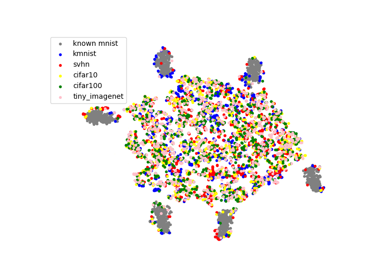
As shown in the first row of Fig.6, in this experiment, known classes come from categories in MNIST, while the remaining categories in MNIST are used as unknown classes, and this data category setting can be seen from the clusters in Fig.6(a). In the Fig.6(b), KMNIST, SVHN, CIFAR10, CIFAR100 and TinyImageNet are used for open set evaluation, and it can be seen from this figure that the network can distinguish the known and unknown classes(open set), except that a few open set data features overlap with known features. In the Fig.6(c), we evaluated the distance distribution of known and unknown features to the center , which corresponds to Fig.6(b). As shown in Fig.6(c), most of the unknown features have smaller distances to the spatial center than the known features.
In the second row of Fig.6, we show the experimental results when the network structure is LeNet++. The distance distribution in Fig.6(e) corresponds to the feature distribution in Fig.6(d). As shown in Fig.6(e), almost all of the unknown features are less distant from the center of feature space than the known features.
The distance analysis results of the two different network structures in Figs.6(c) and 6(e) both prove the view of this paper that unknown features usually tend to be distributed in the center region of the feature space. In addition, although the results of these figures prove our theory, it is obvious that the performance in Fig.6(e) is better than that in Fig.6(c), which may be related to the network architecture and the dimension size of the feature space.
5.5 Further Experiments
Experiment I. All samples from the classes in CIFAR10 are considered as known classes, and samples from ImageNet and LSUN are selected as unknown samplesLSUN. The Settings for data sets are the same as in CROSR, and the other experimental settings are the same as in Section 5.1. The results are shown in Tab.3.
Experiment II. All samples from the classes in MNIST are considered as known classes, and samples from OmniglotOmniglot, MNIST-noise(denoted as M-noise) and Noise are selected as unknown samples. Omniglot is a data set containing various alphabet characters. Noise is a synthesized data set by setting each pixel value independently from a uniform distribution on . M-Noise is also a synthesized data set by adding noise on MNIST testing samples. The Settings for data sets are the same as in CROSR, and the other experimental settings are the same as in Section 5.1. The results are shown in Tab.4.
In these experiments, we can see from the results that on all given datasets, the proposed method is more effective than previous methods and achieves a new state-of-the-art performance. Especially, compared with GCPL, these results once again prove the validity of the constraint term proposed in this paper.
6 Conclusion
As mentioned in this paper, the difficulty of OSR lies in how to reduce the open space risk. To reduce the open space risk, we need to understand why it occurs first. Therefore, this paper explores the direct and root causes of the open space risk. As discussed in section 3, the distribution of known and unknown features determines the open space risk. Because of the mismatch between the unknown class samples and the network convolution kernel, the unknown features usually tend to be distributed in the center region of the feature space. Therefore, it is natural for us to think that if the known features can be distributed in the edge region of the feature space by adjusting the loss function, then the open space risk can be effectively reduced. Based on the above analysis and discussion, we propose the SLCPL loss function. Finally, a large number of experiments and analysis have proved our theory of the open space risk and the effectiveness of our SLCPL.
References
- [1] A. Y. Yang. Robust face recognition via sparse representation – a qa about the recent advances in face recognition and how to protect your facial identity. IEEE Transactions on Pattern Analysis and Machine Intelligence, 31(2):210–227, 2008.
- [2] Alex Graves, Abdel-rahman Mohamed, and Geoffrey Hinton. Speech recognition with deep recurrent neural networks. ICASSP, IEEE International Conference on Acoustics, Speech and Signal Processing - Proceedings, 38, 03 2013.
- [3] Walter Scheirer, Anderson Rocha, Archana Sapkota, and Terrance Boult. Toward open set recognition. IEEE transactions on pattern analysis and machine intelligence, 35:1757–72, 07 2013.
- [4] H. M. Yang, X. Y. Zhang, F. Yin, and C. L. Liu. Robust classification with convolutional prototype learning. In 2018 IEEE/CVF Conference on Computer Vision and Pattern Recognition (CVPR), 2018.
- [5] H. M. Yang, X. Y. Zhang, F. Yin, Q. Yang, and C. L. Liu. Convolutional prototype network for open set recognition. IEEE Transactions on Pattern Analysis and Machine Intelligence, PP(99):1–1, 2020.
- [6] Akshay Raj Dhamija, Manuel Günther, and Terrance Boult. Reducing network agnostophobia. In S. Bengio, H. Wallach, H. Larochelle, K. Grauman, N. Cesa-Bianchi, and R. Garnett, editors, Advances in Neural Information Processing Systems, volume 31. Curran Associates, Inc., 2018.
- [7] J. Walter, Scheirer, P. Lalit, Jain, E. Terrance, and Boult. Probability models for open set recognition. IEEE transactions on pattern analysis and machine intelligence, 2014.
- [8] Lalit P. Jain, Walter J. Scheirer, and Terrance E. Boult. Multi-class open set recognition using probability of inclusion. In David Fleet, Tomas Pajdla, Bernt Schiele, and Tinne Tuytelaars, editors, Computer Vision – ECCV 2014, pages 393–409, Cham, 2014. Springer International Publishing.
- [9] Hakan Cevikalp, Bill Triggs, and Vojtech Franc. Face and landmark detection by using cascade of classifiers. In 2013 10th IEEE International Conference and Workshops on Automatic Face and Gesture Recognition (FG), pages 1–7, 2013.
- [10] Hakan Cevikalp. Best fitting hyperplanes for classification. IEEE Transactions on Pattern Analysis and Machine Intelligence, 39(6):1076–1088, 2017.
- [11] Matthew D. Scherreik and Brian D. Rigling. Open set recognition for automatic target classification with rejection. IEEE Transactions on Aerospace and Electronic Systems, 52(2):632–642, 2016.
- [12] Hakan Cevikalp and Bill Triggs. Polyhedral conic classifiers for visual object detection and classification. In 2017 IEEE Conference on Computer Vision and Pattern Recognition (CVPR), pages 4114–4122, 2017.
- [13] Hakan Cevikalp and Hasan Yavuz. Fast and accurate face recognition with image sets. In 2017 IEEE International Conference on Computer Vision Workshop (ICCVW), pages 1564–1572, 10 2017.
- [14] A. Bendale and T. E. Boult. Towards open set deep networks. In 2016 IEEE Conference on Computer Vision and Pattern Recognition (CVPR), pages 1563–1572, Los Alamitos, CA, USA, jun 2016. IEEE Computer Society.
- [15] Ian Goodfellow, Jean Pouget-Abadie, Mehdi Mirza, Bing Xu, David Warde-Farley, Sherjil Ozair, Aaron Courville, and Yoshua Bengio. Generative adversarial nets. In Z. Ghahramani, M. Welling, C. Cortes, N. Lawrence, and K. Q. Weinberger, editors, Advances in Neural Information Processing Systems, volume 27. Curran Associates, Inc., 2014.
- [16] ZongYuan Ge, Sergey Demyanov, Zetao Chen, and Rahil Garnavi. Generative openmax for multi-class open set classification, 2017.
- [17] Lawrence Neal, Matthew Olson, Xiaoli Fern, Weng-Keen Wong, and Fuxin Li. Open set learning with counterfactual images. In Vittorio Ferrari, Martial Hebert, Cristian Sminchisescu, and Yair Weiss, editors, Computer Vision – ECCV 2018, pages 620–635, Cham, 2018. Springer International Publishing.
- [18] Ryota Yoshihashi, Wen Shao, Rei Kawakami, Shaodi You, Makoto Iida, and Takeshi Naemura. Classification-reconstruction learning for open-set recognition. CoRR, abs/1812.04246, 2018.
- [19] Yandong Wen, Kaipeng Zhang, Zhifeng Li, and Yu Qiao. A discriminative feature learning approach for deep face recognition. In Bastian Leibe, Jiri Matas, Nicu Sebe, and Max Welling, editors, Computer Vision – ECCV 2016, pages 499–515, Cham, 2016. Springer International Publishing.
- [20] Y. Lecun and L. Bottou. Gradient-based learning applied to document recognition. Proceedings of the IEEE, 86(11):2278–2324, 1998.
- [21] Yuval Netzer, Tao Wang, Adam Coates, Alessandro Bissacco, Bo Wu, and Andrew Ng. Reading digits in natural images with unsupervised feature learning. NIPS, 01 2011.
- [22] Alex Krizhevsky. Learning multiple layers of features from tiny images. University of Toronto, 05 2012.
- [23] O. Russakovsky, J. Deng, H. Su, J. Krause, S. Satheesh, S. Ma, Z. Huang, A. Karpathy, A. Khosla, and M. Bernstein. Imagenet large scale visual recognition challenge. International Journal of Computer Vision, 115(3):211–252, 2015.
- [24] Jesse Davis and Mark Goadrich. The relationship between precision-recall and roc curves. In Proceedings of the 23th International Conference on Machine Learning, 2006, volume 06, 06 2006.
- [25] Guangyao Chen, Limeng Qiao, Yemin Shi, Peixi Peng, Jia Li, Tiejun Huang, Shiliang Pu, and Yonghong Tian. Learning open set network with discriminative reciprocal points. In Andrea Vedaldi, Horst Bischof, Thomas Brox, and Jan-Michael Frahm, editors, Computer Vision – ECCV 2020, pages 507–522, Cham, 2020. Springer International Publishing.
- [26] X. Sun, Z. Yang, C. Zhang, G. Peng, and K. V. Ling. Conditional gaussian distribution learning for open set recognition. In Proceedings of the IEEE Conference on Computer Vision and Pattern Recognition, page 13480–13489, 2020.
- [27] Fisher Yu, Ari Seff, Yinda Zhang, Shuran Song, Thomas Funkhouser, and Jianxiong Xiao. Lsun: Construction of a large-scale image dataset using deep learning with humans in the loop, 2016.
- [28] A. Accent. Omniglot writing systems and languages of the world. Zeitschrift Für Psychologie, 175(1):64–91, 1968.