Scheduling of Graph Queries: Controlling Intra- and Inter-query Parallelism for a High System Throughput
Abstract.
The vast amounts of data used in social, business or traffic networks, biology and other natural sciences are often managed in graph-based data sets, consisting of a few thousand up to billions and trillions of vertices and edges, respectively. Typical applications utilizing such data either execute one or a few complex queries or many small queries at the same time interactively or as batch jobs. Furthermore, graph processing is inherently complex, as data sets can substantially differ (scale free vs. constant degree), and algorithms exhibit diverse behavior (computational intensity, local or global, push- or pull-based).
This work is concerned with multi-query execution by automatically controlling the degree of parallelization, with overall objectives including high system utilization, low synchronization cost, and highly efficient concurrent execution. The underlying concept is three-fold: (1) sampling is used to determine graph statistics, (2) parallelization constraints are derived from algorithm and system properties, and (3) suitable work packages are generated based on the previous two aspects. We evaluate the proposed concept using different algorithms on synthetic and real world data sets, with up to 16 concurrent sessions (queries). The results demonstrate a robust performance in spite of these various configurations, and in particular that the performance is always close to or even slightly ahead of the performance of manually optimized implementations. Furthermore, the similar performance to manually optimized implementations under extreme configurations, which require either a full parallelization (few large queries) or complete sequential execution (many small queries), shows that the proposed concept exhibits a particularly low overhead.
1. Introduction
Graph-based data sets (graphs) are continuously increasing in size, with sizes of currently up to multiple billions of vertices and trillions of edges, commonly found in applications including machine learning and data analytics for social and business networks, biology and many other domains. Contrary, other applications like route prediction services for road networks with contention operate on rather small graphs, but have to process many queries concurrently. Additionally, different types of graphs are commonly found: scale-free graphs show a power-law-based degree distribution with a long tail, like social networks, while other graphs can exhibit a rather constant degree among most or all vertices, such as road networks or electrical power grids. Furthermore, the behavior of different graph algorithms can be fundamentally different: while some algorithms, like breadth-first search (BFS), are rather operating on a small subset of the overall graph at a given point in time, algorithms like page rank (PR) operate most of the time on the complete graph. Last, the main objective of a compute system performing graph computations might be unclear at design time: if only single queries are processed, usually latency is the key metric. However, given recent interest in consolidation and hyperscaling, probably the more likely case are large amounts of concurrent queries, which would rather result in throughput being the key metric.
As a result of these orthogonal properties of data and algorithm, it is notoriously difficult to implement high-performance graph computations. While it may be desirable to support multi-query processing, actually even accelerating a single query is difficult. Typical single query optimizations, including algorithm selection (push or pull (Beamer et al. 2012) based with different requirements on atomic operations) and parallelization (Shun and Blelloch 2013; Kulkarni et al. 2007) (multi-threading for faster processing but more memory contention), depend on the properties mentioned before, which are often hard to predict before execution. Contrary, many optimizations come with additional overhead, for instance synchronization for parallel execution, which might diminish the gains or even result in lower performance. Optimizations like NUMA awareness (Zhang et al. 2015) and code generation (Tetzel et al. 2020) can reduce these newly introduced overheads, but are unable to avoid them completely.
For multi-query execution, in the following referred to as number of concurrent queries, the problem worsens as an additional dimension is added, which is to select a schedule with the right amount and set of queries to be processed concurrently. In one of our previous works we showed that multi-query execution using simply multiple parallel engines at the same time can degrade performance (Hauck et al. 2017). To overcome this, given enough concurrent queries ready for execution, a promising option might be to process each query internally sequential (intra-query), what minimizes synchronization overhead, and thereby sourcing the required degree of parallelism from many concurrent queries (inter-query). Another form of multi-query support are solutions that try to share work between different queries as they exist in the literature for relational DBMS (Rehrmann et al. 2020; Psaroudakis et al. 2013a). While such approaches can reduce the overall work, overhead can be substantial if there is nothing to share.
This work gears to optimize multi-query execution by automatically controlling the degree of parallelization at different levels, with overall target metrics including high system utilization, low synchronization costs and highly efficient concurrent execution. We address this problem with resource control system based on knowledge it obtains from the queries that are executed: first, it generates graph statistics by sampling vertices. Second, it takes algorithmic and system properties into account to select certain bounds of parallelization. Last, it generates work packets of certain sizes for execution.
In summary, we hypothesize that the overhead of resource control by efficient statistics generation and simple cost models is outweighed by the improvement of execution. While fundamentally being a trade-off, as perfect statistics and cost predictions would certainly result in optimal execution, efficient methods are required that result in minimal overhead during execution but are still accurate enough for a good scheduling decision. Then, we should observe a highly efficient execution, with i.e. a high number of accumulated operations per time unit, for a variety of scenarios, such as different data (size, type), algorithms (local, non-local), and concurrency (single- or multi-query execution).
In particular, this work makes the following contributions:
- •
An adaptive cost estimation that trades accuracy with overhead based on graph statistics, algorithmic behavior and system properties. In particular, the cost estimator model incorporates traversal behavior estimators (new vertex set, touched memory).
- •
The design and implementation of a runtime resource control system that schedules graph queries during execution based on latency-aware parallelization, cost-based work packaging, and selective sequential execution.
- •
An evaluation based on different algorithms (in total 9 different BFS and PR algorithms), different synthetic and real-world data sets (8 total), and different degrees of concurrent query execution (one to 16 concurrent sessions).
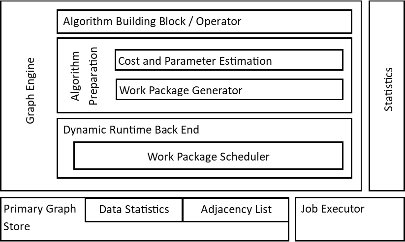
Figure 1 visualizes the overall organization of the proposed system. In the remainer of this work, we will follow up with a section on related work. Section 3 will provide details on the models and estimators that predict graph- and algorithm-dependent behavior ahead of execution. In Section 4, details about the runtime responsible for scheduling decisions during execution will be presented. While up to now, methods and models were not hardware-specific, in Section 5 hardware-specific parameters will be determined. The subsequent Section 6 will provide a detailed evaluation of the proposed method, based on multiple algorithms and their variants, as well as multiple data sets. The last section concludes and provides an outlook on future avenues.
2. Related Work
There is a plethora of related work on graph processing engines and languages, such as Ligra and derived variants (Shun and Blelloch 2013; Dhulipala et al. 2017; Zhang et al. 2015), Galois (Kulkarni et al. 2007), GraphX (Gonzalez et al. 2014), Emptyheaded (Aberger et al. 2017), Green Marl (Hong et al. 2012), and many more for accelerators such as GPUs (Wang et al. 2016) or FPGAs. Commercial representatives include GDBMS like Neo4j11 1 http://neo4j.com and Sparksee22 2 http://www.sparsity-technologies.com. However, such work besides GDBMS is usually focused on providing peak performance for the processing of single, possibly large and time-consuming, graph computations. Instead, our work gears towards concurrent processing of various, possibly small, queries. In the following, we will therefore rather discuss work related to the intrinsic behavior of graph queries and their properties.
In the related work we found several instances that found graph processing inefficiencies. Beamer et al. (Beamer et al. 2015) analyse different graph algorithm and datasets using performance counters. They observe a low compute and bandwidth utilization by the algorithm, but also a high last-level cache (LLC) hit rate that indicates the presence of locality. They also observed that there are diminishing returns for high degrees of multi-threading, which limits its potential.
Several techniques have been proposed that deal with the optimization of structural graph properties on performance. A well-known technique is graph reordering. Balaji and Lucia (Balaji and Lucia 2018) investigate why reordering often does not amortize. They analyze therefore the efficiency of reordering techniques on different data sets and algorithms. They observe among other things that reordering can degrade the performance for push-style operations as it increases false sharing. Finally, they propose a metric called packing factor to decide for hub sorting, if it is worth to reorder a graph.

There are also some works that try to apply a cost-based optimization in the context of graph queries. Bonifati et al. (Bonifati et al. 2018) discuss how classic techniques can be adapted for regular path queries. Based on the assumptions of uniformity of source/target vertex set size, independence of predicates and inclusion of the vertex domains, they demonstrate the adaptation of a synopsis for graphs.
Verstraaten, Varbanescu and de Laat (Verstraaten et al. 2018) analyze BFS variants on different types of graphs in the context of GPU processing. They observe that depending on the graphs different algorithmic variants have an advantage. This effect has also been observed in other works and resulted in approaches like direction-optimized BFS (Beamer et al. 2012). In order to address this issue they propose to use a decision tree based on graph properties, such as size and degree distribution, and runtime properties like the frontier size to switch between different implementations. The decision tree is generated upfront via runs on exemplary data.
Zhang, Yunming, et al. (Zhang et al. 2018) propose a system comprising of a graph DSL and a scheduling language to formulate graph algorithms. While the purpose of the graph DSL is to formulate the algorithm, the scheduling language allows to annotate the DSL with different types of optimizations like push/pull or NUMA mappings. The system is able to apply combinations of these optimizations to the graph algorithm, while guaranteeing that the algorithm is still valid. They also provide an auto tuner, where the system automatically identifies an effective set of optimizations using the elapsed time of the algorithm on the target data.
There also have been proposed approaches, which specifically optimize multi query support. Zhao et. al. (Zhao et al. 2019) address multi query execution by sharing the processed graph data structure between several queries. They therefore process the graph chunk wise and schedule the work of the different queries so that they work on the same chunk that has already been loaded to the LLC. Pan and Li (Pan and Li 2017) try to increase the execution efficiency by scheduling optimization. Via up-front profiling runs of each graph and algorithm pair they estimate the bandwidth requirement and which of two thread counts offers the highest performance. At runtime their system makes sure that only new queries are started with the most effective thread count, if there is available bandwidth not used by other queries.
3. Cost Model and Parameter Estimation
Graph computations respectively their computational iterations notoriously show small elapsed times. Thus, any cost model employed to predict behavior during execution has to exhibit a low overhead, effectively resulting in time required for prediction that is only a fraction of the elapsed time of an iteration of a graph computation. Still, it has to be accurate enough in its predictions to result in reasonable scheduling decisions.
Figure 2 shows an overview of the cost model, consisting of vertex sampling and statistic generation, followed by the selection of thread count and the estimation of static costs per vertex, and the final step of work package generation. In the first part, we will introduce estimators to approximate the size of certain vertex sets, while the second part consists of a cost model for processing vertices including criteria to determine the number of threads for such a processing. In the third part, we show how we derive work packages and thread boundaries from the cost model.
3.1. Traversal Behavior Estimators
For graph traversal algorithms typically the number of starting vertices and processed edges are important cost factors. Besides these often trivially obtainable factors, there are upfront unknown or expensive to obtain factors that have likewise a significant impact on the cost. For our cost modeling two important factors are the number of first time newly visited vertices () in iteration j and the number of vertices that will be touched during iteration j. The to-be-visited vertices are directly related to the found vertices, while touched vertices relate to the amount of memory that is shared, such as duplicate filters during a graph traversal.
There exists no general method to obtain these values exactly without executing the algorithm. In order to estimate them, we model if a vertex is newly visited or touched again as a (conditional) probability process. Our model (cf. Table 1 for the parameters) is based on the general assumption that the probability for all vertices to be visited by an edge is identical. This means there is neither a correlation between different vertices (pure randomness), nor structural effects like the rich club effect (level-dependent), nor is the graph a multigraph (increased probability for some vertices).
| Parameter | Description |
|---|---|
| All vertices in the graph | |
| Vertices that are reachable via a graph traversal (i.e., neither isolated nor without an incoming edge) | |
| Vertices that are touched via edge traversal during each iteration j (cf. Equation 1) | |
| Set of vertices in the current queue at iteration j | |
| Vertices that are newly found after iteration j (cf. Equation 4) | |
| Set of edges traversed by the vertices of the queue | |
| Probability that a vertex will be visited by vertex | |
| Reachable vertices that have not been visited before iteration j | |
| Probability that a vertex has not been visited |
The main idea of our estimation for amount of touched vertices is based on the probability for a reachable vertex to be reached at least once from a vertex from the frontier queue , aggregated for the set of all reachable vertices (cf. Equation 1). As we assume that the graph is not a multigraph and that each outgoing edge of a given vertex is connected to another vertex, so that the probability for a specific vertex to be reached is (cf. Equation 2), with being the out degree of a vertex . It is typically too costly to compute the probability for each vertex of the frontier queue, as the queue can be of substantial size. To reduce these costs, we consider the difference in between the maximum and mean value of outgoing edges per vertex. If this difference is small, then the mean value is used as an approximation (cf. Equation 3), otherwise we extrapolate the product of the probabilities from a sample of vertices in the queue at the beginning of each cost calculation. In this work, we use a simple sampling approach that uses essentially up to the first 8192 vertices as this provides a low latency and sufficient quality.
We approximate also with the number of vertices that are neither isolated nor without an incoming edge. This assumption is based on assumption that the graph forms a single connected component and is purely random. This value is also inexpensive to obtainable during the construction of the adjacency list.
| (1) | ||||
| (2) | ||||
| (3) |
For the estimation of the found vertices , we use a similar approach as for , but besides being reachable the specific vertex needs also to be unvisited (cf. Equation 4). Subsequently, Equation 5 and Equation 6 are derived analogous to before.
| (4) | ||||
| (5) | ||||
| (6) |
3.2. Cost Model
| Parameter | Description |
|---|---|
| Item of generic type, including vertex(), (new) found vertex() or edge() | |
| Set of items of generic type, including set of vertices in the current iteration j queue (), the set of found vertices (), or the set of edges related to the current iteration j queue () | |
| Number of elements in a given set | |
| Number of threads used | |
| Amount of accessed data | |
| Sub-cost of execution for a given item, i.e., processing only vertex or , or edge | |
| Total cost of parallel execution for vertex | |
| Latency of an arithmetic operation | |
| Latency of a non-atomic memory access, depending on the size of the accessed data | |
| Latency of an atomic operation, depending on the size of the accessed data and the amount of threads | |
| Number of arithmetic operations used to process item | |
| Number of memory operations (non atomic load & stores) used to process item | |
| Number of atomic operations used to process item |
In order to model performance (cf. Table 2 for the parameters), we assume that the cost is proportional to the number of vertices that have to be processed, the related edges of these vertices that have to be traversed, and the new vertices that are found as a result of this traversal. Another fundamental assumption is that the parallel and sequential implementations are identical as the parallel code protects critical sections using atomic operations, while the sequential code can instead simply employ plain memory operations. We model this assumption by setting the atomic update latency for a single thread equal to the memory access latency , with both being dependent on the amount of accessed memory .
In general we have three main cost subcomponents: computations (ops), regular memory access operations (mem) and atomic memory operations (atomics). Then, we can formulate the sub-cost for the processing of a given item , as shown in Equation 7.
| (7) | ||||
In order to compare the estimates for the parallel and the sequential case, we use the total cost per vertex . This cost is the sum of the costs to process the vertex itself and the cost of its share of edges and the newly found vertices, as shown in Equation 8.
| (8) | ||||
3.3. Work Package and Thread Boundaries Estimation
| Parameter | Description |
|---|---|
| Start cost for a single thread (typically a few µs) | |
| Minimum work per thread (larger than ) | |
| Start cost for parallel execution (typically a few µs) | |
| Maximum number of cores | |
| Minimum and maximum thread bound | |
| Minimum and maximum thread bound per cache level | |
| Work package set that partitions the work | |
| A work package of a number of vertices that are assigned together to a thread |
In Table 3 we list all parameters related to this section. Based on the cost model, we decide if it is profitable to execute the code in parallel (, see Equation 9), and for which thread ranges () this is true. In detail, the minimum work per work package , the start cost for parallel execution and the start cost per thread are empirically determined, ensuring that the overhead remains reasonable in case of a high load.
The computation of these thread boundaries is expensive, as the thread-count-dependent memory latency is non-linear. In order to do this, we solve the optimization problem for the smallest number of threads () as shown in Equation 10 under some side conditions. For a time-efficient solution, we propose Algorithm 1, in which we continuously double the number of threads and check if we have a valid upper and lower thread bound.
| (9) | ||||
| (10) | ||||
4. System Design
| System Utilization | Synchronization Cost | Concurrent Execution Efficiency | |
|---|---|---|---|
| Latency-aware parallelization | - | ++ | + |
| Cost-based work packaging | ++ | - | 0 |
| Selective sequential execution | - | ++ | ++ |
While, as previously stated, there are three main goals for this work (system utilization, synchronization cost reduction, and concurrent execution efficiency), in detail there are additional requirements:
- •
First, the behavior of the engine has to be predictable. Small changes, like a few extra edges and vertices, should not result in a significantly higher or lower performance, and when code is executed in parallel it should always be faster than a sequential alternative.
- •
Second, the engine needs to be friendly in its resource consumption towards potential other engines. We assume that it is integrated inside of a DBMS along multiple other engines, so the engine cannot assume total control over all system resources.
We use three different techniques to achieve these goals: (1) latency-aware parallelization, (2) cost-based work packaging and (3) selective sequential execution. All of them address the mentioned goals in different ways (cf. Table 4) and are realized by different engine components (cf. Figure 1). In general, the engine is divided into two major components: a preparation component and a runtime component that controls the execution of the core graph algorithm. The idea is to perform a preselection of useful parameters in the preparation step based on data and reasonable assumptions, while the runtime takes care of behavior that is unknown prior to the execution of the algorithm.
4.1. Latency-aware parallelization
In the previous sections we introduced a performance model for graph traversal algorithms. For latency-aware parallelization, we apply this model to our decisions that we take to optimize system parameters. It is realized by the subcomponent Cost and Parameter Estimation in the algorithm preparation step (cf. Figure 1).
In practice it can be observed that different numbers of threads are optimal in terms of performance depending on the primitive operations performed by an algorithm and the size of the intermediate data. Also, in many cases parallel execution can even harm the performance, as too many threads might result in work packages that are too small to compensate overhead costs. Thus, using the cost model we also determine an upper and lower bound for parallel execution of a specific query.
4.1.1. Parameter sets
As shown in Figure 3, we have three different data sources respectively parameter sets to compute the cost:
- (1)
The first type of data are system properties like cache sizes and memory access times, which will be described in Section 5. While many system properties are static, dynamic properties in this work are determined by a single benchmarking run with memoization for future re-use in all queries.
- (2)
The second type are the algorithmic properties like the amount of touched data and the number of operations per edge and vertex, including computations, memory accesses and atomic updates (c.f. in Figure 2). These numbers can be counted and statically set in a descriptor.
- (3)
The third type are statistics about the processed data, such as the frontier queue or the graph, which will be described in the next subsection.
These data sets are combined in a linear model to estimate the resulting memory footprint that is used to determine the cache level the problem can fit into. The determined cache level respectively its latency is in turn used as a parameter for the memory cost model (c.f. in Figure 2). In addition, the level is also used to compute using Algorithm 1 and the related thread boundaries. As the estimated thread boundaries are worst cases, our system works well with contention minimization techniques like small local buffers (Hauck et al. 2019) even without adaptations.
4.1.2. Statistics generation
As stated previously, we need good statistical data related to the vertices we want to process, as the vertex degree and the related work can vary between iterations. In order to not outweigh all benefits, in particular statistics generation has to be of low overhead. An inexpensive way to gather statistical data is to collect them at creation time from the index data structure for the graph topology (adjacency list in Figure 2). Here we can gather statistics for edges and vertices, including the mean and maximum vertex out degrees (cf. , and in Figure 2).
Using these global statistics, we decide at run time if we use global statistics or rather compute local statistics for the current iteration. Here, the indicator is the ratio of maximum vertex degree versus mean vertex degree, as a simple metric to reflect variance. In this work, a threshold of was found to be effective. If we expect a low variance, we compute the cost model parameter for the cost model using global statistics. If we expect a high variance, we compute and on a subset (up to the first vertices) using real vertex degrees and extrapolate global values from this subset. The computation of such statistics is parallelized to minimize overhead.
4.2. Cost-based work packaging
While latency-aware parallelization tries to provide optimal parameters, such as thread count bounds for parallel execution and number of work packages, cost-based work packaging tries to optimize the work packages themselves. On a large scale, the average degree and the related work of sets of vertices can be described statistically. But if the variance of the edge degrees is high, or the number of vertices in a partition is small, the potential work per partition might be non-uniformly distributed between different partitions, resulting in inefficiencies due to the bulk-synchronous execution. Then, some work packages take much longer than others and are executed effectively alone for most of their run time.
We address this problem depending on input data statistics. For cases with a high vertex degree variance and a low numbers of vertices, we generate work packages that are based on the vertex and edge performance model. Therefore, we iterate over the vertices in the frontier and obtain the out degree until we exceed the work share for a particular work package. The number of work packages is limited to a multiple ( times) of the maximum usable level of parallelism to avoid over-parallelization and resulting effects like contention. Finally, we reorder the work packages so that work packages with a high cost due to a single dominating vertex are executed first.
If the number of vertices is high or the variance is low, we still use for efficiency reasons a static partitioning. In addition, the number of work packages is much larger than the used number of cores, allowing the runtime react on dynamic execution behavior.
4.3. Selective Sequential Execution
While the previously mentioned techniques try to generate optimally-sized work packages, they cannot address runtime effects like the dynamic component of contention. To deal with these effects and the fact that in some cases the sequential execution is more efficient, we use as a runtime component a work package scheduler. The work package scheduler has two functions: first, it assigns work to the worker threads; second, it controls if the work is executed sequentially or in parallel.
When the execution of a task starts, the runtime requests worker threads from the system according to the upper thread boundary. When a worker gets assigned, it registers itself with the scheduler and requests a work package. The scheduler checks if the number of registered workers is higher than the minimum boundary for parallel execution. If this is true, it assigns a work package to these workers for parallel execution. If the condition is false, it assigns one worker to execute a package sequentially, while the other threads wait until the package is completed. Then, the scheduler reevaluates the worker situation. This is repeated for a limited number of sequential packages after which the scheduler releases all but one thread and completes the execution sequentially.
This approach avoids a central scheduler that needs to deal with many different tasks, which might run a very short time and might be of different type, such as relational and graph combined. It executes also the tasks using an optimal parallelism strategy, taking into account concurrently executed tasks. Especially for scenarios with concurrent queries, it can be observed that sequential execution of a single query is preferable over parallel execution of a single query, which follows intuition as such would easily result in over-parallelization.
4.4. Interaction of the subcomponents

The different interactions in between the subcomponents are summarized in Figure 3, in particular how the result of one subcomponent is used in the succeeding one and how certain boundaries are set. The preparation step of the Cost Estimator provides information for latency-aware parallelization and therefore about the most-suited execution mode. Cost-based work packaging (Package Generator) provides the work packages that fulfill the assumption of equal work distribution, but also maintains a sufficient amount of work per package. The runtime in the end (Dynamic Scheduler) uses these information for the selective sequential execution, while it also takes into account dynamic system behavior, which is not considered by the previous two subcomponents.
The figure furthermore summarizes which properties of system, algorithm, and data are taken into consideration by which subcomponent. Also, different lines highlight the flow of information, with dashed lines highlighting access to upfront prepared date, solid lines highlight data flow between component, and dotted line highlighting data for the next iterations. Principally, it is also possible that some stage provides feedback like the measured cost of a work package as shown by the dotted line from dynamic scheduler to cost estimator. This might allow to optimize later iterations of the graph algorithm, however, for this work we considered this out of scope.
4.5. Implementation
The complete system was implemented using C++, a HANA graph engine derived system (Hauck et al. 2015) and HANA’s job execution framework (Psaroudakis et al. 2013b). The algorithms have been implemented using two lambda functions, one sequential and one parallel. We run the preprocessing for the execution depending on the type of algorithm: for topology-centric algorithm like Page Rank, where the vertices stay the same for all iterations, we run it once; for data-driven algorithm like BFS, we run it for every iteration as for every iteration a different set of vertices is processed.
For the used data that is not obtained during the preprocessing steps, we have different sources: We obtained the algorithmic properties by counting the respective operations used and memory touched by the lambdas and stored them for each algorithm as metadata. In a productive system a query compiler could do the counting automatically. The graph data statistics are gathered during the construction of the adjacency list. Dynamic system properties like memory access latency are determined prior to experiments using the degree count benchmark. Similarly, static system properties like cache sizes are determined also prior to experiments using appropriate tools such as CPUID.
5. Modeling Update Contention
While in general the compute cores of a multi-core system are independent, in reality resources like the CPU’s internal interconnection network (system interconnect), some cache hierarchies, or the memory controller are shared among these cores. Furthermore, some modules are limited in parallelism (e.g., banked caches), or even require serialization (e.g., memory controller). Typically a shared use of resources increases contention and thus the delay of a particular operation. As a result, the CPU has to wait longer until an operation like a memory access or a data transfer completes.
A special case of this resource contention is the use of the same memory address by multiple cores. Read-only access to a range of addresses causes virtually no contention as multiple shared copies of a given memory address can be installed in different caches. However, shared copies are not allowed in the case of a write access, thus write operations typically result in a large amount of invalidations, subsequent cache misses, and ultimately contention. The same applies to atomic operations like mutually exclusive read-modify-write operations, which even intensify the problem as corresponding cache lines will be locked during the operation and no other requests on the same cache line will be served.
Especially for memory sensitive algorithms, like many graph algorithms, memory contention has a significant impact on overall performance. In general there are many sources on different levels that influence contention and its impact on the overall performance: on hardware level, there are (non-conclusive) the CPU cores, system interconnects, memory accesses, cache organization and the specification and implementation of atomic operations. On software level, there are low-level sources like thread-to-physical-core mapping and high-level sources like the algorithmic design. Push-based graph algorithms are typically prone to contention as they update the same address, while pull-based algorithm are not. Furthermore, the data that is being processed can be a source of contention, and between all of these sources there are complex interactions that are highly dynamic in nature.
5.1. Update Latency Estimation Under Contention
In practice, the aforementioned sources make it hard to model contention and how it affects latency and throughput of updates. Essentially, to predict and optimize the performance of parallel graph algorithms, an accurate prediction of update performance is necessary. Our solution is to omit analytical modeling of contention entirely, and instead create a simple model based on experiments and measurements. Thus, the general idea is to train a parametric model on a given system using a reference algorithm and differently sized data sets. Such a training is required any time a new hardware configuration is used, however, the training process is to a large extend automated. We assume that Little’s law applies and throughput and latency are interchangeable. To later predict the latency of a given update, we map it to our reference problem.
As a reference algorithm we select degree count, because its parameters can be varied almost arbitrarily to model different scenarios. Furthermore, it is comparable to many push-based graph algorithms. This algorithm counts the occurrence of vertex IDs of the vertex set in an edge list, either as source or target vertex, using fetch-and-add atomic operations on a single counter array. When executed in parallel, the input edge list is partitioned in non-overlapping parts of 16k edges each. If this results in fewer partitions than cores, we exclude this setting from the experiments. These partitions are dynamically dispatched as work packages to a set of worker threads.
The reference data set should be of a type that causes high contention, and furthermore should be representative and not of pathological nature. Thus, RMAT is chosen as being representative for many graph problems. The scale-free degree distribution of RMAT graphs causes high contention on vertices with high degree count. Furthermore, contention varies with the number of vertices and the related counter array size, as memory accesses will be accordingly distributed.
In our measurements, we focus on two different parameters: first, the total number of threads, and second, the amount of touched memory, which is the unique set of shared addresses accessed by any memory operation. To ensure that thread counts are representative with regard to later use in inference, the thread count used here for experimentation is the total number of threads successively divided by two, so that modeled thread counts are exponentially spaced.
In this regard, with being a single counter of the counter array, the amount of touched memory, e.g., the counter array size is:
| (11) |
5.2. Measurements and Derived Heuristics
Experimental results in Figure 5 show that update time is mainly a function of . This particularly holds true as we vary the data type of a single counter (). Therefore, we see no dependency to graph parameters like the number of vertices or edges, which allows us to limit experimentation to counter array size and to generalize from this measurement. As a result, we obtain a set of measurements describing the mean update time, respectively latency , which is a function of memory set size and number of threads .
An additional observation we make in Figure 5 is that with an increasing the update time decreases as the contention is distributed across more memory locations. This effect seams to be rather a function of the logarithm of the counter array size than depending linearly on the counter array size.
To derive a suitable heuristic that predicts for a given data set size and thread count , we first identify bounds for the memory access costs. As cache levels are discrete, we use the highest memory hierarchy level that can fit the data set of size , i.e. , with being the capacity of memory hierarchy level . To approximate the effective access latency, we use a polynomial interpolation between the cache level and , with the rationale that higher cache levels will also observe some cache hits. While this holds true for referring to main memory (note that we exclude , referring to main memory), for a special case is required. In this case, the problem fits into L1 cache, thus we set , effectively an identical lower and upper bound.
Then, describes the polynomial interpolation, depending on data set size . Note that we use the logarithm of the data set size, according to the observation made in Figure 5.
| (12) |
The difference in between the latency of the two memory hierarchy levels and , with derived from as shown above, is:
| (13) |
Last, the update time prediction is a function of the access cost of the lower bound , but effectively reduced by multiplied with the previous interpolation cubed:
| (14) |
While cubed seems non-intuitive, it is empirically derived from experiments on multiple systems and showed the best fit in a couple of different regressions. We leave a detailed understanding of this behavior for future work, but observe that the found best fit is inline with our observation that modeling update contention is complicated. In this sense, the present fit is no surprise.
Another important factor for the update time prediction are dynamic effects that depend on the number of threads. For the estimators in Section 4, we need thread-dependent estimations, such as atomic update latency, only for the threads that we measure. In Figure 5 we see that there is a clear dependency between the number of threads and the atomic update time. Furthermore, we also see is that when limiting the problem to higher cache levels (by adapting problem size), thread count has a much higher impact on atomic update time. To address this dependency, we estimate the atomic update time using the measured access times with the anticipated number of threads.
6. Evaluation
In the following, we evaluate the proposed runtime system based on PageRank (PR) and Breadth-First Search (BFS) algorithms, respectively various variants thereof. As a test system, we use a two socket system equipped with Intel Xeon E5-2660 v4 processors, each with 14 cores and Hyper-Threading enabled, 35 MB last-level cache for each socket, and 128 GB DDR4 RAM.
PR has been evaluated as a topology-centric algorithm variant using two different types (push, pull). In the push variant the updates to compute the ranks are pushed to the target vertices, which requires in our parallel implementations for each update an atomic operation. The pull variant gathers data from all source vertices to compute a rank, which does not require atomic operations. For an analysis of these different types, see (Whang et al. 2015). BFS represents the data-driven algorithm and is implemented in a top-down variant.
Both algorithms, PR and BFS and their variants are in addition realized using different schedulers (sequential, simple parallel, scheduler): Sequential executes the code completely sequential. Simple parallel executes the code in parallel using a simple work partitioning that partitions the frontier queue in equal sized packages. The package size is determined by the maximum number of threads and a lower limit. The scheduler variant uses our proposed scheduler. In particular, sequential variants will serve in concurrent query settings as a baseline, as under high concurrency a per-query sequential processing is usually preferable.
We measure the whole execution of a full PR run after the creation of the adjacency list and its dictionary, from the setup of all supporting data structures until the algorithm converges and the result vector can be returned. Twenty-four times the number of concurrent sessions repeated full PR runs are executed and measured, and we report mean throughput in Processed Edges per Second (PEPS). The BFS algorithm has been executed from different start points and measured 50 times the number of concurrent sessions, so we report the throughput derived from the mean of these measurements in Traversed Edges per Second (TEPS).
Furthermore, as the behavior of graph computations is highly data-dependent, we cover synthetic data sets based on RMAT with different scale factors (SF), as well as real-world data sets, such as soc-Live-Journal1, as-skitter, roadNet-CA, cit-Patents, roadNet-PA, web-BerkStan, and soc-pokec-relationships from the Stanford Large Network Dataset Collection (Leskovec and Krevl 2014).
6.1. Evaluation of single query performance to identify scheduling overhead
While the intent of the proposed scheduling is to optimize concurrent query execution, we focus in this subsection on single query performance mainly for overhead analysis. In Figure 7 we report performance scaling for different PR implementations across RMAT graphs of different scale factors. We observe that single-query PR performance depends on problem size and algorithm, although pull versions seem to be preferred. Principally, push and pull algorithms have completely different properties, therefore also differ in their cost models. Furthermore, we observe that sequential processing is faster for small problem sizes ( for push and for pull), otherwise parallel processing is preferable.
We can assess the overhead of the proposed scheduling method by comparing it to sequential to avoid an unrealistic perfect selection of parameter for simple parallel. In this regard, we observe that for the pull-based algorithms, the scheduler makes always the right choice to execute the code in parallel, which prohibits an analysis of the overhead. Comparing scheduler push with sequential push, we see that for a long time the scheduler variant behaves like the sequential variant with only a small (3% at SF17 - 30% at SF12) reduction in performance. Thus, in spite of fundamental differences between push and pull variants, in particular with regard to the use of atomics, the scheduler chooses the right execution strategy, so that the overhead never dominates the elapsed time.
Furthermore, we evaluate the performance of different PR implementations on different types of graphs in Figure 7. We observe that for different data sets and single query PR, the difference between simple push and its scheduling-optimized counterpart scheduler (push) is negligible, with either one having only small advantages compared to the other, depending on the data set. The difference for pull variants behaves similarly, even though here for one data set there is a substantial advantage for the scheduler variant. Thus, for PR it is apparent that our scheduler is stable across different data sets, and that the scheduling overhead is small.
Regarding Breadth-First Search (BFS), results for RMAT graphs of different scale factors are reported in Figure 9. Similar to PR, data set size determines algorithm choice: for , sequential processing is fastest, otherwise simple (parallel) and scheduler are almost equally faster. As a reminder, similar to PR, simple is a straight-forward range partitioning of the frontier queue, while scheduler is based on our proposed scheduler. This experiment particularly highlights that these scheduling optimizations come with virtually negligible overhead in comparison to simple parallelization. Only for small data sets, sequential query processing is faster, still our scheduler is performing better than simple in this regime. One reason is that our scheduler reduce false invalidation as they reduce concurrent writes to the same memory locations.
We also assess BFS performance on real-world data sets, as reported in Figure 9. For single query execution, BFS performance is highly data-dependent. In particular, scheduler can be slower than simple, which is based on naive parallelization, albeit with only small differences and almost only if the difference to sequential is substantial. Presumably, scheduling overhead is virtually constant while BFS processing time is highly dependent on the data set. Thus, for a small BFS execution time, scheduling overhead can become more dominant. Furthermore, results suggest that data sets resulting in low performance (roadNet-CA,-PA) prefer scheduler over simple, probably due to complex dependencies (edges) and little parallelization opportunities. As a result, scheduler is always close to the best algorithm, independent of particular data set characteristics.
In summary, we observe that scheduling overhead seems to be small to negligible, and that sometimes the scheduling optimizations are actually even beneficial for overall performance. As expected, graph computations are highly dependent on algorithm and data, thus performance results, both in absolute and relative terms, are also highly dependent on this tuple. In this regard, it is noteworthy to point out that performance of our scheduler is stable across the various evaluated tuples of algorithm variant and data set.
6.2. Concurrent query performance on synthetic RMAT data
We continue by evaluating the performance scaling across multiple sessions for different PR algorithms, as shown in Figure 10. Different scale factors are covered by different subfigures. We observe that scheduler pull is by far fastest, although the advantage depends on data set size and concurrency (number of sessions). Only for a small data set size (SF 16) and a high number of sessions, sequential pull is faster as these data sets provide very little opportunities for parallelism. Furthermore, results show that the break-even point in between these two moves to larger amounts of concurrency with increasing data set size. With increasing data set size the still existing overhead of parallel execution becomes more negligible.
Figure 11 reports results from similar experiments for BFS on RMAT data. For small data set sizes, sequential processing is by far the fastest, in particular with growing concurrency. As it can be seen in figure 9 our scheduler chooses for the small data set parallel execution as it underestimates the contention. While for medium sized data sets simple parallel is slightly fastest, with growing data set size our scheduler becomes advantageous. This is mainly in line with expectations, as too small data set sizes result in parallel processing being rather inefficient.
6.3. Concurrent query performance on real-world data
We complete our experiments by evaluating concurrent queries on data, which is probably most representative for real-world applications. We start with PR as reported in Figure 12. Overall, it is apparent that scheduler pull is dominantly fastest, independent of data set and concurrency. While its performance is almost constant with regard to concurrency, performance of alternatives (in particular sequential push and sequential pull) is usually scaling linearly with concurrency. This suggests that for some data sets, in particular roadNet-CA/-PA and web-BerkStan, sequential alternatives can reach the performance of the scheduler implementation given sufficient concurrency. However, for other data sets, such as cit-Patents or soc-pokec-relationships, the performance increase by concurrency for sequential seems to be too low to reach the scheduler implementation. A reason for this behavior is the different internal level of parallelism that these data sets allow.
Performance of BFS on real-world data under concurrent execution is reported in Figure 13. Algorithm performance is highly dependent on data set and concurrency, basically forming four patterns:
- (1)
For soc-LiveJournal1 and soc-pokec-relationships, simple parallel and our scheduler are almost equally fast, with sequential substantially slower. However, the difference decreases with increasing concurrency, suggesting that concurrency higher than evaluated might result in a break-even point.
- (2)
For as-skitter, cit-Patents and web-BerkStan, performance of the three alternatives is almost equal but with high variance depending on concurrency. If sequential is much slower, the difference will decrease with growing concurrency, sometimes even outperforming the other algorithms.
- (3)
With regard to the previous pattern, we have to report that as-skitter is a rather special case as the overall speed is very high. As a result, the overhead is of particular importance.
- (4)
For roadNet-CA and roadNet-PA, sequential and our scheduler are almost equally fast, with small advantages for sequential, and scaling is almost linear with concurrency. Simple parallel has a constant performance, resulting in a growing gap with increasing concurrency.
As a result, we observe that for both PR and BFS the use of our scheduler result in executions that are most efficient, being close to the best performing alternative or even ahead of it. In detail, for PR, scheduler pull or scheduler push are substantially faster than alternatives, while for BFS, our scheduler is close or ahead of sequential or simple parallel performance.
7. Conclusion
Considering scalable computing systems, both in the cloud and on-premise, there is a strong trend towards consolidation of resources. As a result, solutions that are too specialized for a particular task or situation are no longer appropriate, as the overall workload characteristics change to being highly variant in terms of concurrency, workload type, and data set.
In this work, we address some of these needs by presenting a system that focuses on the overall throughput especially when there are multiple active queries. It increases the overall throughput by controlling the degree of parallelism in each query to reduce the overall synchronization overhead.
The system is split in two parts: a proactive preparation step and a reactive runtime component. On one side the preparation step estimates the upcoming work for the next iteration and prepares the work in package form for the runtime. The estimates are based on multiple sources that include information about the system and the algorithm, but also information that is gathered from the processed data. On the other side the runtime uses the prepared information and combines them with runtime information like the available threads. Together it uses them to execute the graph algorithm sequential or parallel in an efficient way.
In our experiments, we showed that our approach provides a robust performance for different types of graphs (social network, web graphs road network) and algorithm (BFS, push and pull PR) without the need for manual adjustments of runtime parameters. The system chooses depending on the circumstances the most effective way to execute a graph algorithm, so that achieved performance is near the optimum. For multi-query execution we showed that the system is able to efficiently handle multiple queries at the same time. For queries with high internal parallelism it keeps the performance constant, while it achieves performance gains with an increasing number of queries when the internal parallelism is low.
Acknowledgements.
We would like to thank our colleagues Marcus Paradies and Romans Kasperovics for their support.References
- (1)
- Aberger et al. (2017) Christopher R. Aberger, Andres Nötzli, Kunle Olukotun, and Christopher Ré. 2017. EmptyHeaded: Boolean Algebra Based Graph Processing. arXiv:1503.02368 [cs.DB]
- Balaji and Lucia (2018) Vignesh Balaji and Brandon Lucia. 2018. When is Graph Reordering an Optimization?. In IEEE International Symposium on Workload Characterization (IISWC).
- Beamer et al. (2012) Scott Beamer, Krste Asanovic, and David Patterson. 2012. Direction-optimizing breadth-first search. In SC’12: Proceedings of the International Conference on High Performance Computing, Networking, Storage and Analysis. IEEE, 1–10.
- Beamer et al. (2015) Scott Beamer, Krste Asanovic, and David Patterson. 2015. Locality exists in graph processing: Workload characterization on an ivy bridge server. In Workload Characterization (IISWC), 2015 IEEE International Symposium on. IEEE, 56–65.
- Bonifati et al. (2018) Angela Bonifati, George Fletcher, Hannes Voigt, and Nikolay Yakovets. 2018. Querying graphs. Synthesis Lectures on Data Management 10, 3 (2018), 1–184.
- Dhulipala et al. (2017) Laxman Dhulipala, Guy Blelloch, and Julian Shun. 2017. Julienne: A framework for parallel graph algorithms using work-efficient bucketing. In Proceedings of the 29th ACM Symposium on Parallelism in Algorithms and Architectures. 293–304.
- Gonzalez et al. (2014) Joseph E Gonzalez, Reynold S Xin, Ankur Dave, Daniel Crankshaw, Michael J Franklin, and Ion Stoica. 2014. Graphx: Graph processing in a distributed dataflow framework. In 11th USENIX Symposium on Operating Systems Design and Implementation (OSDI 14). 599–613.
- Hauck et al. (2017) Matthias Hauck, Marcus Paradies, and Holger Fröning. 2017. Can Modern Graph Processing Engines Run Concurrent Queries Efficiently?. In Proceedings of the 5th International Workshop on Graph Data-management Experiences & Systems(GRADES). ACM, 5.
- Hauck et al. (2019) Matthias Hauck, Marcus Paradies, and Holger Fröning. 2019. Software-based Buffering of Associative Operations on Random Memory Addresses. In 33rd IEEE International Parallel & Distributed Processing Symposium (IPDPS).
- Hauck et al. (2015) Matthias Hauck, Marcus Paradies, Holger Fröning, Wolfgang Lehner, and Hannes Rauhe. 2015. Highspeed graph processing exploiting main-memory column stores. In European Conference on Parallel Processing. Springer, 503–514.
- Hong et al. (2012) Sungpack Hong, Hassan Chafi, Edic Sedlar, and Kunle Olukotun. 2012. Green-Marl: a DSL for easy and efficient graph analysis. In Proceedings of the seventeenth international conference on Architectural Support for Programming Languages and Operating Systems. 349–362.
- Kulkarni et al. (2007) Milind Kulkarni, Keshav Pingali, Bruce Walter, Ganesh Ramanarayanan, Kavita Bala, and L. Paul Chew. 2007. Optimistic parallelism requires abstractions. SIGPLAN Not. (Proceedings of PLDI) 42, 6 (2007), 211–222. https://doi.org/10.1145/1273442.1250759
- Leskovec and Krevl (2014) Jure Leskovec and Andrej Krevl. 2014. SNAP Datasets: Stanford Large Network Dataset Collection. http://snap.stanford.edu/data.
- Pan and Li (2017) Peitian Pan and Chao Li. 2017. Congra: Towards efficient processing of concurrent graph queries on shared-memory machines. In 2017 IEEE International Conference on Computer Design (ICCD). IEEE, 217–224.
- Psaroudakis et al. (2013a) Iraklis Psaroudakis, Manos Athanassoulis, and Anastasia Ailamaki. 2013a. Sharing Data and Work Across Concurrent Analytical Queries. Proceedings of the VLDB Endowment 6, 9 (2013).
- Psaroudakis et al. (2013b) Iraklis Psaroudakis, Tobias Scheuer, Norman May, and Anastasia Ailamaki. 2013b. Task scheduling for highly concurrent analytical and transactional main-memory workloads. In 4th International Workshop on Accelerating Data Management Systems Using Modern Processor and Storage Architectures (ADMS).
- Rehrmann et al. (2020) Robin Rehrmann, Carsten Binnig, Alexander Böhm, Kihong Kim, and Wolfgang Lehner. 2020. Sharing opportunities for OLTP workloads in different isolation levels. Proceedings of the VLDB Endowment 13, 10 (2020), 1696–1708.
- Shun and Blelloch (2013) Julian Shun and Guy E Blelloch. 2013. Ligra: a lightweight graph processing framework for shared memory. In Proceedings of the 18th ACM SIGPLAN Symposium on Principles and Practice of Parallel Programming. 135–146.
- Tetzel et al. (2020) Frank Tetzel, Wolfgang Lehner, and Romans Kasperovics. 2020. Efficient Compilation of Regular Path Queries. Datenbank-Spektrum 20, 3 (2020), 243–259.
- Verstraaten et al. (2018) Merijn Verstraaten, Ana Lucia Varbanescu, and Cees de Laat. 2018. Mix-and-Match: A Model-driven Runtime Optimisation Strategy for BFS on GPUs. In 2018 IEEE/ACM 8th Workshop on Irregular Applications: Architectures and Algorithms (IA3). IEEE, 53–60.
- Wang et al. (2016) Yangzihao Wang, Andrew Davidson, Yuechao Pan, Yuduo Wu, Andy Riffel, and John D Owens. 2016. Gunrock: A high-performance graph processing library on the GPU. In Proceedings of the 21st ACM SIGPLAN Symposium on Principles and Practice of Parallel Programming. 1–12.
- Whang et al. (2015) Joyce Jiyoung Whang, Andrew Lenharth, Inderjit S Dhillon, and Keshav Pingali. 2015. Scalable data-driven pagerank: Algorithms, system issues, and lessons learned. In European Conference on Parallel Processing. Springer, 438–450.
- Zhang et al. (2015) Kaiyuan Zhang, Rong Chen, and Haibo Chen. 2015. NUMA-aware graph-structured analytics. In Proceedings of the 20th ACM SIGPLAN Symposium on Principles and Practice of Parallel Programming. 183–193.
- Zhang et al. (2018) Yunming Zhang, Mengjiao Yang, Riyadh Baghdadi, Shoaib Kamil, Julian Shun, and Saman Amarasinghe. 2018. GraphIt: a high-performance graph DSL. Proceedings of the ACM on Programming Languages 2, OOPSLA (2018), 121.
- Zhao et al. (2019) Jin Zhao, Yu Zhang, Xiaofei Liao, Ligang He, Bingsheng He, Hai Jin, Haikun Liu, and Yicheng Chen. 2019. GraphM: an efficient storage system for high throughput of concurrent graph processing. In Proceedings of the International Conference for High Performance Computing, Networking, Storage and Analysis. 1–14.