Floer homology, twist coefficients, and capping off
Abstract.
For an open book decomposition , the fractional Dehn twist coefficients are rational numbers measuring the amount that the monodromy twists the surface near each boundary component. In general, the twist coefficients do not behave nicely under the operation of capping off a boundary component. The goal of this paper is to use Heegaard Floer homology to constrain the behavior of the fractional Dehn twist coefficients after capping off. We also use our results about fractional Dehn twists to study the Floer homology of cyclic branched covers over fibered two-component links.
1. Introduction and Statement of Results
Let be an open book decomposition with boundary components for a closed, oriented 3-manifold and denote by the fractional Dehn twist coefficient along , as defined in [HKM07]. Roughly, measures twisting near after applying . In this paper, we will not define fractional Dehn twist coefficients directly, but instead reference a few key properties:
Theorem 1.1 ([KR13],[IK17],[HKM07]).
.
- (1)
- (2)
- (3)
If the contact structure supported by is tight, then
- (4)
If then for any arc leaving we have
where denotes signed intersection number in an annular neighborhood of .
- (5)
If then for any arc leaving we have
Now, let denote the open book decomposition obtained by capping off with a disk and extending to the identity along the capping disk. This capping off procedure defines a cobordism
where is obtained from by Dehn surgery along with framing given by that of the pages of the open book decomposition, and is the trace of the surgery.
The cobordism often admits a natural symplectic structure ([GS12], [Wen13]), and hence provides a natural operation between the contact structures and . Nonetheless, the invariants and (which provide valuable information regarding and , respectively) often differ greatly.
For example, Baldwin and Etnyre in [BE12] provide examples of genus 1 open books with two boundary components, where the fractional Dehn twist coefficients of are arbitrarily positive, and the fractional Dehn twist coefficients of are arbitrarily negative. We revist these examples in Section 4.
One difficulty in constraining the change in fractional Dehn twist coefficients under capping off is that the dynamical structure of may change globally in unpredictable ways. This is related to the fact that the Nielsen–Thurston type of may differ from that of , and ultimately reflects the complexity of the mapping class groups of surfaces.
1.1. L-space case
Unless explicitly stated otherwise, all Heegaard Floer groups will take coefficients in . The simplest form of our main result is as follows:
Theorem 1.2.
Let be an open book for an L-space . If either:
- (1)
, or
- (2)
and for some ,
then in .
If has two components, note that is connected. In this case, we can use a result of Honda–Kazez–Matić from [HKM08] (which was later repoven by Conway in [Con19]), that when , to obtain a numerical bound on the change in fractional Dehn twist coefficients:
Corollary 1.3.
Let be an open book for an L-space with boundary components. If either:
- (1)
, or
- (2)
for both
then .
The bound in the above corollary can also be used fairly easily to obstruct from being an L-space. For example, if the contact structure associated to is tight, is psuedo-Anosov, and , then is not an L-space. In Section 4, we use this idea to show that the ambient manifolds associated to many genus one, two boundary component open books (including the Baldwin–Etynre examples) are not L-spaces.
1.2. Non-L-space case
When is not an L-space, Theorem 1.2 can be generalized as follows:
Theorem 1.4.
If is a rational homology sphere and either:
- (1)
, or
- (2)
and for some ,
then .
Note that in this general case, we require that is a rational homology sphere, which is unnecessary when is an L-space.
Because adding Dehn twists around to does not change , and adding positive/negative Dehn twists corresponds to surgery with respect to the page framing, we have the following immediate corollary:
Corollary 1.5.
If is a rational homology sphere and then, for all ,
As in the previous subsection, when has boundary components, it follows that is connected. Hence, we can get a numerical bound on in this case, too:
Corollary 1.6.
Let be an open book for with boundary components . If is a rational homology sphere and either:
- (1)
, or
- (2)
and ,
then .
Using the results above, we can easily obtain lower bounds on the reduced Floer homology of the ambient manifold of an abstract open book. In general, a precise calculation of the Heegaard Floer homology of an arbitrary manifold is hard to ascertain directly, and our results provide a simple bound on the complexity. See section 4 for some examples.
1.3. Floer homology of branched covers
Given an open book for , we can consider the branched cyclic cover with open book decomposition for any . We then have the following corollary regarding the Floer homology of , which we prove in Subsection 4.1:
Corollary 1.7.
Let be an open book for with boundary components , such that and . Then:
- •
is not an L-space for some , and
- •
if is sufficiently large and is a rational homology sphere, then
This corollary can be seen as a partial generalization of Corollary 5 of [HM18] to the case of a two-component link. Addditionally, Kalelkar and Roberts demonstrate in [KR15] the existence of taut foliations on for sufficiently large . This is enough to obstruct from being an L-space for some , but leaves open the question of the minimal such . The work of the present paper provides an easily computable numerical approximation of , and of .
1.4. Ingredients for the proofs
The relationship between Floer homology and twist coefficients was previously studied by Hedden and Mark in [HM18]. They showed that if has connected boundary , then is an upper bound for . Our results can be interpreted as a generalization of Hedden and Mark’s work to the significantly more complicated case of open books with disconnected boundary.
When is connected, the surface is closed and hence is no longer an open book decomposition. Nonetheless, describes a fibered 3-manifold given by the mapping torus of , which is obtained by page-framed surgery along .
Hedden and Mark’s construction relies on a key fact about this fibration which was originally proved by Ozsváth and Szabó in [OS05]: there is a class
such that the map
associated to the capping off cobordism satisfies
The idea behind the strategy of Hedden and Mark is to use this fact, in conjunction with a surgery-exact triangle of Ozsváth–Szabó (see [OS01]), to study the non-vanishing of the contact class after adding boundary Dehn twists. In place of the class for the fibered 3-manifold , we will use the contact class of the capped-off open book , and a similar argument to that of Hedden and Mark.
The key ingredient to our argument in the L-space setting is the following naturality result, which we prove in Section 2:
Proposition 1.8.
When , the map
satisfies . In particular, there is a unique -structure on so that , and for any .
Naturality of the contact class under capping off was originally studied by Baldwin in [Bal13], where he proved a weaker form of naturality in the -structure , when is a rational homology sphere. Note that our result applies to the full map, and does not require that is a rational homology sphere.
Proof of Theorem 1.2.
Suppose that is an L-space and . We then know that , and is not in the image of for some fixed sufficiently large . Now, consider the Ozsváth–Szabó surgery-exact triangle:
Note that by assumption (in either Case (1) or (2) of Theorem 1.2), we have:
Hence, by Proposition 1.8, we have .
Because is an L-space, every element in is in the image of . Because the map is -equivariant, it follows that is contained in the image of , too. In particular, is not in the image of . By exactness, it follows that is not in the kernel of , so .
To prove Theorem 1.4, we need some more machinery. Nonetheless, the proof is similar in spirit to that of Theorem 1.2. The major difference is that when is not an L-space, is no longer completely contained in the image of . To rectify this, we would like to use to bound the part of not contained in , but this idea will require a different surgery-exact triangle and a modification to the contact class . See Section 3 for more details.
Acknowledgements.
I am greatly appreciative of my advisor John Baldwin for suggesting this topic, and for his patience, support and guidance in the preparation of this work. His mentorship over the past two years has been invaluable.
2. The proof of Proposition 1.8

Right: Heegaard diagram corresponding to an open book with the intersection point shown. A diagram for replaces the left-most curve with a pushoff of , shown in green.
In the presence of an open book decomposition , there is a natural Heegaard splitting for given by:
Note that if has genus and boundary components, then has genus , and we may see the attaching curves explicitly on in terms of the monodromy as follows:
Let be a basis of arcs for (i.e. for and is a disk). For all , let be obtained from by an isotopy in the direction specified by the orientation of , so that and intersect transversely and positively exactly once. We may then define the attaching curves and on by (see Figure 1 for reference):
In order to define the Floer homology groups, we must additionally specify a basepoint on the Heegaard surface. To do this, note that the complement of the and curves in consists of two small triangles with boundary on , and for each as well as a large “outer” region with boundary intersecting all the and . We place the basepoint in this large outer region.
Let be the unique intersection point on between and , and note that the pointed Heegaard diagram describes the manifold . The collection thus defines an element of the Heegaard Floer chain group whose homology is the group .
Theorem 2.1 ([HKM09],[OS05]).
The generator is a cycle whose homology class is an invariant of the contact structure , called the “contact class” and denoted by . And, when is overtwisted, .
From the Heegaard diagram for , we can also describe a pointed Heegaard diagram for as follows. Choose as above. For the attaching curves, choose for all and for exactly as before, and let be a copy of the boundary component . See Figure 1 for reference.
Then, Theorem 2.1 implies that the collection is a generator for in , where is the unique intersection point between and . Additionally, is a pointed Heegaard triple diagram representing the cobordism (after perturbing away from by a small isotopy for , as on the right of Figure 2).

Middle: Another non-standard triangle (2yellow+orange) near .
Right: Standard triangles near for .
Lemma 2.2 ([Bal13]).
The Heegaard triple diagram is admissible, and therefore yields a well-defined map
The map is defined by counting Whitney triangles with vertices on intersection points , , and , where is a top dimensional generator. For , let denote the standard trianglular domain connecting and , shown in gray in Figure 2.
Lemma 2.3 ([Bal13]).
Let be a homotopy class of Whitney triangles connecting , and some intersection point . If has a holomorphic representative with , then for , and
where is a triangular domain in with vertices at , and .
The key point of the proof of Proposition 1.8 is that the number of possible triangular domains appearing in the Heegaard triple is given by the integer part of the fractional Dehn twist coefficient . In particular, they are all of the form show in yellow or 2yellow+orange, on the left and middle in Figure 2, respectively.
Lemma 2.4.
Let , and suppose is a homotopy class of Whitney triangles with a holomorphic representative and , connecting , , and some intersection point . Then, and

Right: A Whitney triangle connecting , and with and .
Proof.
By Theorem 2.3, we know , so it suffices to show that and . Recall that for such a triangular domain , the necessary boundary conditions are as depicted in Figure 3 on the right, ignoring the point (which will be used in a later section).
Note that is the only intersection point between and in , and that is the only triangular domain with the proper boundary conditions connecting , and . Hence, it suffices to show that there are no intersection points in with a triangular domain connecting , and satisfying the proper boundary conditions.
To show this, first note that we may consider only domains contained in an annular neighborhood of . And, because of the relative positions of and on , we can see that and must intersect negatively on at .
Because , we know that on by Theorem 1.1. Reversing orientation then yields on . Note that because starts to the right of on , we must have:
on . Because is by definition an integer, it follows that and therefore intersects positively (or not at all) with in an annular neighborhood of on . Moreover, near the boundary, we may remove bigon regions to guarantee that intersects only positively (or not at all) with in an annular neighborhood, so that there are no negative intersection points. It follows that there are no triangular domains satisfying the necessary boundary conditions and ending on an intersection point . ∎
3. The proof of Theorem 1.4
When is not an L-space, the situation becomes much more complicated: in the proof of Theorem 1.2, if is not an L-space, the image of may not be contained in the image of . To rectify this, we will use to bound the rank of the image of not contained in the image of for sufficiently large .
This idea will require an argument using “twisted coefficients” in the group ring as in [HM18], where is the cyclic group of order . The first task is to describe the -coefficient system of interest.
Using the construction of the previous section, we start with pointed Heegaard diagrams for and for . Additionally, choose a marked point on the curve isotopic to the capped-off in (see Figure 1 for reference). We then define the Heegaard Floer chain group with -coefficients by:
where is the number of times that crosses the basepoint (see the left of Figure 3 for reference). We can then define the “twisted” Heegaard Floer homology group by taking the homology of this chain complex.
Hedden and Mark used a similar variant of Heegaard Floer homology with -coefficients in [HM18], where they extended the Ozsváth–Szabó surgery-exact triangle. For our purposes, their result may be stated as:
Theorem 3.1 ([HM18]).
There is an exact triangle:
where and are -equivariant, and is defined on the chain-level by:
for any .
In the theorem, is defined similarly for Whitney triangles as it is for Whitney disks, and it may be helpful to see Figures 3 and 2 for reference. For example, the triangular domain on the left of Figure 2 has , the domain in the middle has , and the domain on the right has .
For more details on -coefficients, we direct the reader to the original paper [HM18], and for more details on “twisted coefficients” in general, see [AP10] or [OS01].
Using this construction and Lemma 2.4, we can prove an analogue of Proposition 1.8 for the map appearing in the Hedden–Mark exact triangle.
Proposition 3.2.
If , then the map defined in Theorem 3.1 satisfies:
Proof.
Note that caps off to for any , and consider the pointed Heegaard triple diagram for the capping off cobordism applied to .
If , then . In particular, by Lemma 2.4, there is a unique homotopy class of Whitney triangles with , and no Whitney triangles in with for any . Now, note that and , and the result follows. ∎
The goal of the proof of Theorem 1.4 is to use the Hedden–Mark exact triangle, together with 3.2, to show that the open book supports a tight contact structure. But, as mentioned in the beginning of this section, we will need to use the bound on the size of the part of not contained in the image of to conclude this.
To do that, we would like to compare the rank of the submodule generated by , to the rank of . The following two lemmas will help with this comparison:
Lemma 3.3.
If , then the classes for all , and for sufficiently large .
Proof.
If , then it follows that the full untwisted invariant in is non-zero, and is not in the image of for some fixed which is sufficiently large.
Consider the -linear coefficient map
given by . This map is clearly -equivariant, and we can see that for all . Because , it follows that , too. Similarly, if for some , it follows that by -equivariance of , which is a contradiction. This shows that for all , and . ∎
Lemma 3.4.
If is a rational homology sphere and , then .
Proof.
We’ll show by way of contradiction that are linearly independent over . The goal of the proof is to use a hypothetical dependence relation to find disks crossing some prescribed number of times, and take a linear combination of the (domains of the) disks to produce a periodic domain with . To such a , we can then associate a singular homology class by capping off the boundary curves with disks in the and handlebodies. Note that if , then is nontrivial and consequently . Because is a rational homology sphere, we have , so this would yield a contradiction. Thus, if we can produce such a , the proof is complete.
Now, suppose we have an -dependence relation:
and set . Because for all by Lemma 3.3, we have . By definition, there is a chain with .
We can write where for all , and for some chains . Because for all , again by Lemma 3.3, we know that for all , too.
Now, if appears as a summand of for any with , then we have two disks and from to , with and . We can then take , which is a periodic domain, and nontrivial because . This would yield a contradiction, as described above.
So, we may reindex to match with the index set , i.e. , where , , and . Moreover, does not appear as a summand of for any , so we may simply assume does not appear as a summand of for any .
We now have:
Because does not appear as a summand of for any , the equation above forces . In particular, there are an even number of copies of for each . Because in homology for all , it follows that the chains for all , too. So, we may write where and .
Since there are an even number of copies of for each , we can guarantee there are an even number of copies of for each . In particular, for each , there are and with and disks from to , respectively, with and . Additionally, for each , we have a disk from to with . We can then choose any and take . Observe that is a periodic domain with , and hence nontrivial.
∎
Remark.
It is worth mentioning that one can prove, using an argument similar to that of [HKM09], that the submodule is the contact submodule studied by Hedden and Mark in [HM18]. A similar argument to that of the proof above shows that this submodule is either rank 0 or rank over when is a rational homology sphere.
We are now ready to prove Theorem 1.4. The reader is encouraged to compare the proof to that of Theorem 1.2, recorded in Subsection 1.4.
Proof of Theorem 1.4.
Fix , and consider the Hedden–Mark exact triangle from Theorem 3.1:
By assumption, we have (in either case (1) or (2) of Theorem 1.4), so it follows that . Thus, by Proposition 3.2:
Because , Lemma 3.3 implies that for some fixed sufficienlty large . By the -equivariance of , it follows that the preimage is contained in , where is the map in the Hedden–Mark exact triangle above. Because additionally is a rational homology sphere, we can conclude from Lemma 3.4 that . By definition of and , we have:
so cannot be contained in the image of . Because , by exactness we must then have in .
4. Applications
4.1. Floer homology of branched covers
Given an open book for and any , we may form the cyclic branched cover over the binding (thought of as a link in ) by taking the ambient manifold of the open book . Note that the diffeomorphisms and are isotopic (rel. boundary) on , so the open book is well-defined.
Proof of Corollary 1.7.
If and , we can choose sufficiently large that and simultaneously. For this choice of (and all larger), Corollary 1.3 implies that is not an L-space.
For the rank bound, when we further assume is a rational homology sphere, Corollary 1.6 implies that:
for sufficiently large. Hence, . ∎

4.2. Lower bounds on from abstract open books
Using Theorem 1.4 and Corollary 1.6, we can quickly find lower bounds on when is the ambient manifold of an open book with two binding components.
Example 4.1.
Let , and be the curves on the surface depicted in Figure 4, and define . Let , and consider the open book , which was originally studied by Baldwin and Etynre in [BE12]. As mentioned in [BE12], is pseudo-Anosov by a construction of Penner [Pen88]: if is a collection of filling curves on , where the curves in and in are pairwise disjoint, then any product of positive Dehn twists along and negative Dehn twists along is pseudo-Anosov. Note that this same construction also shows that is pseudo-Anosov.
The same method as in Example 4.1 can be used to bound the reduced Floer homology for the ambient manifolds of many different open books on a suface with genus and boundary components. For example:
Example 4.2.
Using the same notation as above, note that any open book on can be written as a product:
If , and , , and for all , then one can calculate that , and . As in the previous example, both and are pseudo-Anosov by Penner’s construction [Pen88]. It follows that, if and is a rational homology sphere, then . In particular, whenever and , then is not an L-space.
This same idea can also be easily applied to open books of higher genus which are given as a product of boundary Dehn twists with symmetric mapping classes.
5. Further Directions and Questions
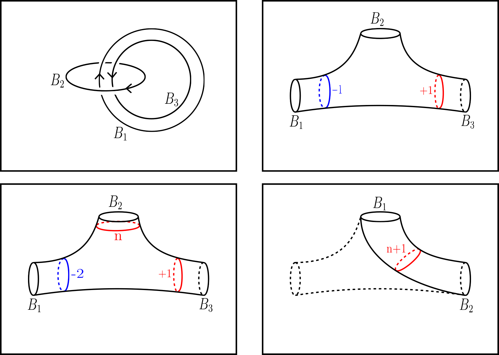
Bottom left: The open book . Bottom right: The open book .
The results above provide a universal upper bound for the fractional Dehn twist coefficient of a capped-off open book with connected binding, given that the un-capped fractional Dehn twist coefficients are negative enough. We would like to be able to extend our results to open books with more than two boundary components, but this is difficult in general. The following example demonstrates that even for the simplest case of three boundary component, planar open books in lens spaces, we have no clear bound:
Example 5.1.
Let be the connect sum of a negative and positive Hopf link in , as in Figure 5. This link is fibered, with open book where is a pair of pants. The page framing on is the Seifert framing, so we may add arbitrary Dehn twists along to obtain a family of open books for . This changes the page-framing on to with respect to the Seifert framing, so we can add another negative Dehn twist along to obtain an open book for the lens space , where . Note that .
On the other hand, capping off now yields the open book where is a core curve of the annulus . The ambient manifold for is the Lens space which is a rational homology sphere, and we can see that for .
Indeed, there is a significant technical challenge to applying the same strategy outlined in the previous section: we don’t have an analogue of the relationship between twist coefficients and reduced Floer homology for open books with disconnected binding. In fact, as noted by Baldwin and Etynre in [BE12], the open books of Example 4.1 provide an infinite family of examples with genus and boundary components where , despite the fractional Dehn twist coefficients on both boundary components being arbitrarily large.
This leads us to the following question:
Question 5.2.
Is there a way to guarantee that in terms of fractional Dehn twist coefficients when has boundary components?
In another direction, our results involve heavy restrictions on the fractional Dehn twist coefficient of an open book along the boundary component being capped off. However, one may intuitively wonder about a restriction on the amount that the twist coefficient can change along a fixed boundary component, independent of the others, in terms of the Floer homology of the underlying manifold.
Question 5.3.
Can we bound the change in twist coefficient of a fixed boundary component, independent of the twist coefficient of the boundary component which is being capped off?
Finally, our results only give a universal upper bound of for the twist coefficient of the capped off open book, independent of the twist coefficients along for . One may intuitively hope to get a bound on the difference between the twist coefficients, in terms of the Floer homology:
Question 5.4.
When has boundary components, can we bound the difference in terms of the Floer homology of ? What about when ?
References
- [AP10] Yinghua Ai and Thomas D. Peters. The twisted floer homology of torus bundles. Algebr. Geom. Topol., 10(2):679 – 695, 2010.
- [Bal13] John A. Baldwin. Capping off open books and the ozsváth-szabó contact invariant. J. Symplectic Geom., 11(4):521–561, 2013.
- [BE12] John A. Baldwin and John Etnyre. Admissible transverse surgery does not preserve tightness. Mathematische Annalen, 357, 03 2012.
- [Con19] James Conway. Tight contact structures via admissible transverse surgery. Journal of Knot Theory and Its Ramifications, 28, 02 2019.
- [GS12] David T. Gay and András I. Stipsicz. On Symplectic Caps, pages 199–212. Birkhäuser Boston, Boston, MA, 2012.
- [HKM07] Ko Honda, William H Kazez, and Gordana Matić. Right-veering diffeomorphisms of compact surfaces with boundary. Invent. Math., 169:427–449, 2007.
- [HKM08] Ko Honda, William H Kazez, and Gordana Matić. Right-veering diffeomorphisms of compact surfaces with boundary II. Geom. and Top., 12(4):2057 – 2094, 2008.
- [HKM09] Ko Honda, William H. Kazez, and Gordana Matić. On the contact class in heegaard floer homology. J. Differential Geom., 83, 2009.
- [HM18] Matthew Hedden and Thomas E. Mark. Floer homology and fractional dehn twists. Adv. in Math., 324:1–39, 2018.
- [IK17] Tetsuya Ito and Keiko Kawamuro. Essential open book foliation and fractional dehn twist coefficient. Geom. Dedicata, 187, 2017.
- [KR13] William H. Kazez and Rachel Roberts. Fractional dehn twists in knot theory and contact topology. Algebr. Geom. Topol., 13(6):3603–3637, 2013.
- [KR15] Tejas Kalelkar and Rachel Roberts. Taut foliations in surface bundles with multiple boundary components. Pacific Journal of Mathematics, 273:257–275, 02 2015.
- [OS01] Peter Ozsvath and Zoltan Szabo. Holomorphic disks and three-manifold invariants: Properties and applications. Annals of Mathematics, 159, 06 2001.
- [OS05] Peter Ozsváth and Zoltán Szabó. Heegaard floer homology and contact structures. Duke Math J., 129(1):39–61, 2005.
- [Pen88] R. C. Penner. A construction of pseudo-anosov homeomorphisms. Trans. Amer. Math. Soc., 310(1):179–197, 1988.
- [Wen13] Chris Wendl. Non-exact symplectic cobordisms between contact 3-manifolds. Journal of Differential Geometry, 95(1):121 – 182, 2013.