跳到论文正文
W Papers独立论文阅读器 arXiv:2110.10518 论文正文 计算阅读时间 · 0%
引用这篇论文根据当前论文元数据生成,正式投稿前建议核对。


License: arXiv.org perpetual non-exclusive license
arXiv:2110.10518v1 [stat.ML] 20 Oct 2021

Online non-parametric change-point detection
for heterogeneous data streams observed over graph nodes

Alejandro de la Concha    Argyris Kalogeratos    Nicolas Vayatis
Abstract

Consider a heterogeneous data stream being generated by the nodes of a graph. The data stream is in essence composed by multiple streams, possibly of different nature that depends on each node. At a given moment τ\tau, a change-point occurs for a subset of nodes CC, signifying the change in the probability distribution of their associated streams. In this paper we propose an online non-parametric method to infer τ\tau based on the direct estimation of the likelihood-ratio between the post-change and the pre-change distribution associated with the data stream of each node. We propose a kernel-based method, under the hypothesis that connected nodes of the graph are expected to have similar likelihood-ratio estimates when there is no change-point. We demonstrate the quality of our method on synthetic experiments and real-world applications.

Introduction

Change-points delimit segments in which a data stream exhibits a notion of stationarity. Their detection is fundamental for time-series analysis and control tasks. Modern challenges include handling larger amounts of more complex data streams, a clear example of which is when those lie over a graph. Many real-world systems can be seen as a network in which each node generates a stream of data. For instance, activity or monitor data can be collected from users in a social network, stations in a railway, or banks in a financial system. A change-point in these systems may signify the shift of users’ interest, a disruption of the railway service, or the early signs of an economic crisis. Using any available information to detect as fast as possible such changes is important. The aim of this paper is to address the naturally arising question: how can we integrate the latent information carried by the graph structure in a change-point detection task?

Related work. Change-point detection methods can be classified into offline (Truong, Oudre, and Vayatis 2020; Aminikhanghahi and Cook 2016) and online approaches (Tartakovsky, Nikiforov, and Basseville 2014; Tartakovsky 2021) depending on whether we have access to a complete dataset or we observe data in near real-time. Further classification can be done into parametric, semi- and non-parametric approaches, depending on the assumptions which are made regarding the distribution generating the data stream. The Online Kernel Graph Detector (OKGD) presented in this paper is a online non-parametric approach.

Kernel methods have been used in both the offline (Harchaoui, Moulines, and Bach 2009; Garreau and Arlot 2018; Arlot, Celisse, and Harchaoui 2019) and the online settings (Kawahara and Sugiyama 2012; Bouchikhi et al. 2019; Li et al. 2019), showing useful theoretical and practical properties. Kernel-based methods are appealing because they can be applied to complex data and monitor different kinds of changes, such as mean shifts, or changes in the correlation between variables. More related to our work is the kernel-based algorithm presented in (Kawahara and Sugiyama 2012) that estimates directly the likelihood-ratio between the post-change-point and the pre-change-point probability density function of a data stream. A change is spotted as soon the estimator is bigger than a given threshold. Its theoretical properties under a semi-parametric hypothesis are analyzed in (Kanamori, Suzuki, and Sugiyama 2012).

The existing literature has hardly studied change-point detection for heterogeneous data streams, where each node may generate a stream of different dimensions and/or nature (e.g. some nodes may generate sensor signals, others text or other content, etc.). To the best of our knowledge, (Ferrari and Richard 2020) is the only paper referring to this setting. Its authors make the hypothesis that the underlying graph has a community structure and a change may occur in only one of these communities at a given moment. Using tools originating from Graph Signal Processing (Ortega et al. 2018; Perraudin and Vandergheynst 2017), they spot the change-point and the affected community. Their approach consists in estimating independently the likelihood-ratio for each of the nodes. This essentially composes a graph signal, which is then filtered with the Graph Fourier Scan Statistic (GFSS) (Sharpnack, Rinaldo, and Singh 2016) in order to detect the community of interest. The main disadvantage of this approach is its limited applicability to cases where the graph has poor community structure (e.g. graphs approximating a manifold structure). Furthermore, the sophistication of GFSS is limited, as it is a graph filter whose only effect is to filter out the high frequencies while maintaining the low frequencies. Therefore, scenarios where changes may concern nodes that are less concentrated at a site of the graph (or even arbitrary to it) is a blind spot to this approach.

Main contributions. In this paper we present the Online Kernel Graph Detector (OKGD) algorithm that builds upon the notion graph smoothness, which formalizes the intuition that two nodes are expected to have a similar behavior if they are connected. We introduce a kernel-based cost function made of two terms: a penalized LSE-like term aiming to infer the likelihood-ratio at each of the nodes, and a Laplacian penalization term aiming to guarantee the smoothness of the estimations. Then, we develop a stochastic gradient descent strategy to minimize the cost function.

In a nutshell, the OKGD approach: i) is online, ii) non-parametric, meaning it is flexible and can handle heterogeneous data streams, ii) exploits the expected smoothness of the graph signal derived by the likelihood-ratio estimations, and iv) is easy to parallelize and its computational time improves with the sparsity of the graph.

Notation and definitions

Let xix_{i} be the ii-th entry of vector xx, and Ai​jA_{ij} be the entry associated with the ii-th row and jj-th column of a matrix. 𝟏N\mathbf{1}_{N} represents the vector with NN ones (resp. 𝟎N\mathbf{0}_{N}), and 𝕀N\mathbb{I}_{N} is the N×NN\times N identity matrix (the subscript may be omitted). Let G=(V,E,W)G=(V,E,W) be a weighted and undirected graph without self-loops, where VV is the set of vertices, EE the set of edges, and W∈N×NW\in\real^{N\times N} its adjacency matrix.

Let us suppose we observe NN synchronous data streams that could be of different nature, each of them being generated by a node of GG. We denote by yv,ty_{v,t} the observation generated by node vv at time tt, by yt=(y1,t,…,yN,t)y_{t}=(y_{1,t},...,y_{N,t}) the vector obtained after concatenating all the observations from all the nodes at time tt. We will denote by Y={yt}t∈{1,…}Y=\{y_{t}\}_{t\in\{1,...\}} the whole time-series.

Additionally, we suppose that the graph GG (hence WW) remains constant through time. We also suppose that WW is weighted and symmetric, Wu​v=Wv​uW_{uv}=W_{vu}, and each Wu​vW_{uv} entry is a positive value reflecting how similar are expected to be the data streams generated by the nodes uu and vv (note: Wu​u=0,∀u∈VW_{uu}=0,\forall u\in V). The degree of vv is dv=∑u∈ng​(v)Wu​vd_{v}=\sum_{u\in\text{ng}(v)}W_{uv}, where u∈ng​(v)u\in\text{ng}(v) means that uu is a neighbor of vv.

A term that we use throughout the paper is that of graph signal which is attributed to any function x:V→ℝx:V\rightarrow\R defined from the nodes of a graph into ℝ\R. Consider as change-point the timestamp at which the distribution associated with a time-series changes meaning its probability density function (p.d.f.) goes from p⁡(y)p(y) to p′​(y)p^{\prime}(y). Here, a change-point is denoted by τ\tau, which indicates a change in the marginal distribution of a subset of nodes CC, more explicitly:

{t<τyv,t∼pv​(y);t≥τyv,t∼pv′​(y),\left\{\begin{array}[]{ll}t<{\tau}\ \ y_{v,t}\sim p_{v}(y);\\ t\geq{\tau}\ \ y_{v,t}\sim p_{v}^{\prime}(y),\end{array}\right. (1)

where pv​(y)≠pv′​(y)p_{v}(y)\neq p^{\prime}_{v}(y) if v∈C{v\in C}, otherwise pv​(y)=pv′​(y)p_{v}(y)=p^{\prime}_{v}(y). We consider pv​(y),pv′​(y)p_{v}(y),p^{\prime}_{v}(y) as well as CC and τ\tau o be unknown. We denote by p⁡(y)p(y) (resp. p′​(y)p^{\prime}(y)) the joint p.d.f. of YY before the change-point (resp. after the change-point), meaning its vv-marginal p.d.f. is pv​(y)p_{v}(y) (resp. pv′​(y)p^{\prime}_{v}(y)). A simple example of this framework is illustrated in Fig. 1.

Similarly, we denote by 𝔼p⁡(y)​[⋅]\mathbb{E}_{p(y)}[\cdot] (resp. 𝔼p′​(y)​[⋅]\mathbb{E}_{p^{\prime}(y)}[\cdot]) the expected value under the pre-change (resp. post-change) distribution. For a set of observations {yt}t∈I\{y_{t}\}_{t\in I} in a given time interval II, we denote by 𝔼(p​(y),p′​(y))​[⋅]\mathbb{E}_{(p(y),p^{\prime}(y))}[\cdot] the expectation on the joint p.d.f. of the time-series at that interval. If there is a change, then p​(y)≠p′​(y)p(y)\neq p^{\prime}(y), otherwise p​(y)=p′​(y)p(y)=p^{\prime}(y).

In this work, we estimate and monitor the likelihood-ratio between pv′​(y)p^{\prime}_{v}(y) and pv​(y)p_{v}(y) at each node, that is the quantity rv​(t)=pv′​(y)pv​(y)r_{v}(t)=\frac{p^{\prime}_{v}(y)}{p_{v}(y)}. We define by r⁡(y)=(r1​(y),…,rN​(y))r(y)=(r_{1}(y),...,r_{N}(y)) the vector whose entries are the likelihood-ratios corresponding to each node of GG. Note that r⁡(y)r(y) is a graph signal. In the text, we call null hypothesis the case where there is no change, i.e. when pv​(y)=pv′​(y)p_{v}(y)=p^{\prime}_{v}(y), ∀v∈V\forall v\in V, which opposes the alternative hypothesis where a change exists.

The smoothness of a graph signal xx over a graph GG can be defined using a Laplacian operator ℒ{\mathcal{L}} associated with GG. Here, we use the combinatorial Laplacian operator, ℒ=diag⁡(dv)v∈V−W{\mathcal{L}}=\operatorname{diag}(d_{v})_{v\in V}-W, for which smoothness is defined as:

s⁡(x)=x𝖳​ℒ​x=12​∑u,v∈VWu​v​(xu−xv)2.{}s(x)=x^{\mkern-1.5mu\mathsf{T}}{\mathcal{L}}x=\frac{1}{2}\sum_{u,v\in V}W_{uv}(x_{u}-x_{v})^{2}. (2)

s⁡(x)s(x) is always positive, and is lower when adjacent values are more similar.
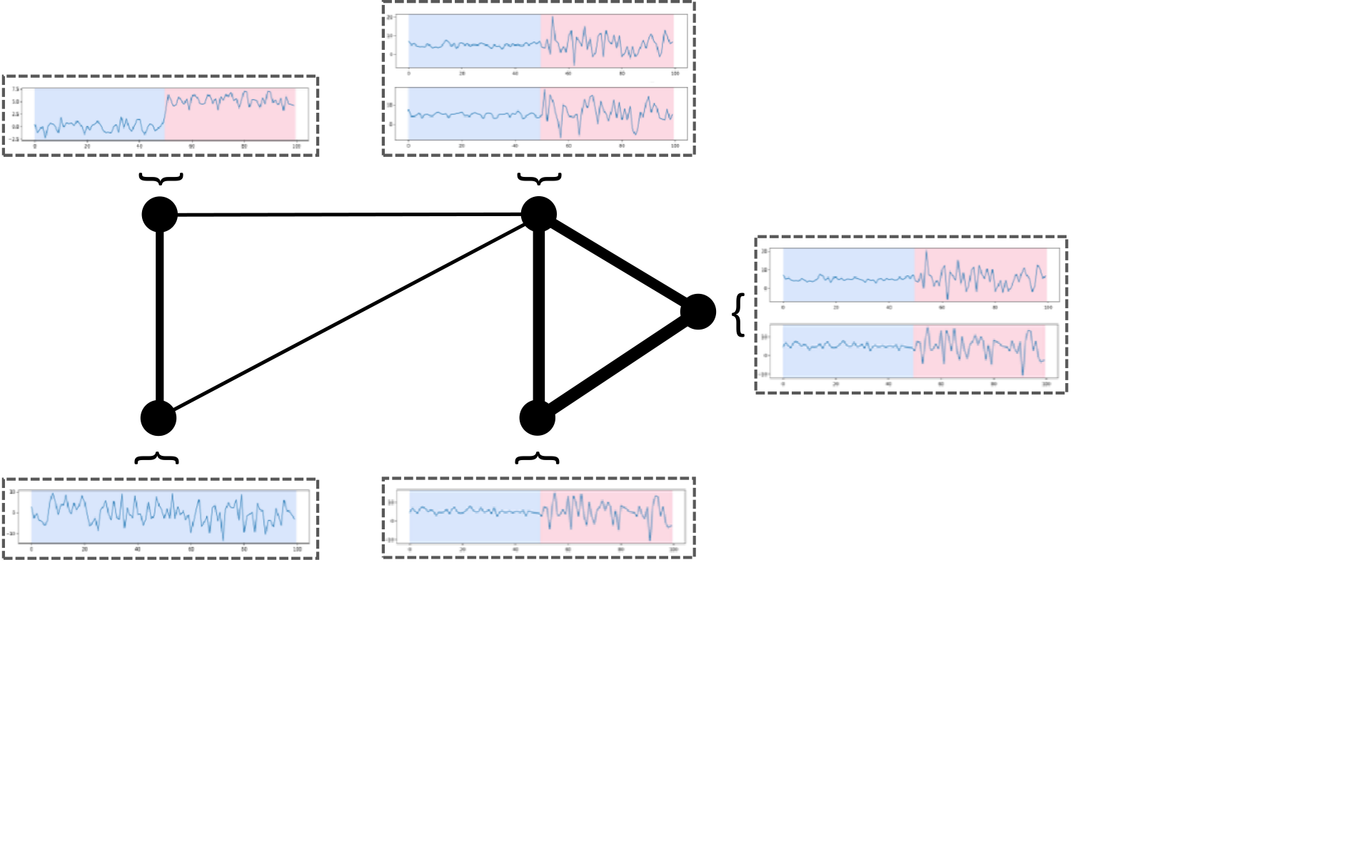
Refer to caption
Figure 1: Example of a heterogeneous data stream, observed over the nodes of a weighted graph that expresses node behavior similarity. The dimensions or even the nature of the time-series of each node may vary. A change occurs in a subset of nodes and the change-point is at the moment when the color changes in the respective time-series. For the top-left node, the change-point is associated with a shift in the mean, while the three nodes of the clique on the right present a shift in the variance of their streams.

Problem formulation and solution

Our approach relies on a cost function that would estimate the likelihood-ratio rvr_{v} associated with each node, and would integrate all such estimates. We desire the solution of the cost-function to have a similar behavior to that of rvr_{v} under the null hypothesis, so that we can detect when new observations come from a different probabilistic model. Furthermore, we want to be able to solve the optimization problem in a way that allows the online update of the parameters.

Estimating the likelihood-ratio rvr_{v} at each node vv requires a dictionary and a kernel function associated with vv. In our approach, the estimation of the rvr_{v}’s of all nodes is performed jointly, however we suppose that a dictionary and a kernel function can be defined and learned independently for each node. The quality of the dictionary affects the performance of the algorithm. This is why we propose to integrate the approach of (Richard, Bermudez, and Honeine 2009) in order to enlarge our dictionary with arriving observations that are dissimilar to what has been previously observed.

Cost function

Most usually we do not know the form of the joint p.d.f.’s, before the change-point p⁡(y)p(y) and after it p′​(y)p^{\prime}(y); same for its marginals pv​(y)p_{v}(y) and pv′​(y)p^{\prime}_{v}(y) for each node vv. Instead, our method uses a kernel-based approach to estimate the graph signal g⁡(y):r⁡(y)−𝟏N=(r1​(y1)−1,…,r⁡(yN)−1)𝖳g(y):r(y)-\mathbf{1}_{N}=(r_{1}(y_{1})-1,...,r(y_{N})-1)^{\mkern-1.5mu\mathsf{T}}. Under the null hypothesis of no change-point, it holds g⁡(y)=𝟎Ng(y)=\mathbf{0}_{N}, hence s⁡(g⁡(y))=0s(g(y))=0, see Eq. 2). For this reason, in our cost function we include a penalization term against the non-smoothness of g⁡(y)g(y):

Φ⁡(g)\displaystyle\Phi(g) =𝔼p⁡(y)​[‖r⁡(y)−𝟏N−g⁡(y)‖222+λ2​g​(y)𝖳​ℒ​g​(y)]\displaystyle=\mathbb{E}_{p(y)}\left[\frac{\left\lVert r(y)-\mathbf{1}_{N}-g(y)\right\rVert_{2}^{2}}{2}+\frac{\lambda}{2}g(y)^{\mkern-1.5mu\mathsf{T}}{\mathcal{L}}g(y)\right] (3)
=12​𝔼p⁡(y)​[‖g⁡(y)‖22]+𝔼p⁡(y)​[𝟏N𝖳​g​(y)]−𝔼p′​(y)​[𝟏N𝖳​g​(y)]\displaystyle=\frac{1}{2}\mathbb{E}_{p(y)}[\left\lVert g(y)\right\rVert_{2}^{2}]+\mathbb{E}_{p(y)}[\mathbf{1}_{N}^{{\mkern-1.5mu\mathsf{T}}}g(y)]-\mathbb{E}_{p^{\prime}(y)}[\mathbf{1}_{N}^{{\mkern-1.5mu\mathsf{T}}}g(y)]
+λ4​𝔼p⁡(y)​[∑u,v∈VWu​v​(gu​(y)−gv​(y))2]+K,\displaystyle+\frac{\lambda}{4}\mathbb{E}_{p(y)}\left[\sum_{u,v\in V}W_{uv}\left(g_{u}(y)-g_{v}(y)\right)^{2}\right]+K,

where KK is a constant. Notice that the initial expression of Eq. 3 works under the distribution p⁡(y)p(y) before the change-point (null hypothesis) and consists of a least square term that controls the approximation error, and a penalization term aiming to promote the smoothness of g⁡(y)g(y). Then, the second equality is due to 𝔼p⁡(y)​[rv​(y)​gv​(y)]=𝔼pv′​(y)​[gv​(y)]\mathbb{E}_{p(y)}[r_{v}(y)g_{v}(y)]=\mathbb{E}_{p^{\prime}_{v}(y)}[g_{v}(y)], which is is easy to verify given the definition of r⁡(y)r(y).

The next step is to approximate Φ⁡(g)\Phi(g) by means of empirical expectations. It is common that a user has a sample of npren^{{\text{pre}}} observations generated by the probabilistic model p⁡(y)p(y), then npostn^{{\text{post}}} new observations arrive and she has to decide if those last observations are still coming from p⁡(y)p(y). We denote by YtY_{t} the set of all observations coming from p⁡(y)p(y) and have occurred up to the decision time tt, and YtpostY_{t}^{{\text{post}}} the last observations that need to be validated. Let us suppose that the user takes a sub-sample Ytpre⊆YtY_{t}^{{\text{pre}}}\subseteq Y_{t} of size npren^{{\text{pre}}}, and observes npostn^{{\text{post}}} recent observations up to time tt:

{Ytpre={y1,…,ynpre},∀y1,…,ynpre∼p⁡(y);Ytpost={yt−npost,…,yt−1,yt}.\left\{\begin{array}[]{ll}Y_{t}^{{\text{pre}}}&=\{y_{1},...,y_{n^{{\text{pre}}}}\},\ \forall y_{1},...,y_{n^{{\text{pre}}}}\sim p(y);\\ Y_{t}^{{\text{post}}\!\!\!\!}&=\{y_{t-n^{{\text{post}}}},...,y_{t-1},y_{t}\}.\end{array}\right. (4)

We can now define our optimization problem in terms of its empirical expected values:

min(g1,…,gN)∈H1×H2,…,×HN∑v∈V[∑yj∈Ytpregv2​(yv,j)2​npre\displaystyle\min_{(g_{1},...,g_{N})\in H_{1}\times H_{2},...,\times H_{N}}\sum_{v\in V}\left[\frac{\sum_{y_{j}\in Y_{t}^{{\text{pre}}}}g^{2}_{v}(y_{v,j})}{2n^{{\text{pre}}}}\right. (5)
+(∑yj∈Ytpregv​(yv,j)npre−∑yj∈Ytpostgv​(yv,j)npost)]\displaystyle\left.+\left(\frac{\sum_{y_{j}\in Y_{t}^{{\text{pre}}}}g_{v}(y_{v,j})}{n^{{\text{pre}}}}-\frac{\sum_{y_{j}\in Y_{t}^{{\text{post}}}}g_{v}(y_{v,j})}{n^{{\text{post}}}}\right)\right]
+λ2​[∑yj∈Ytpre∑u,v∈VWu​v​(gv​(yv,j)−gv​(yu,j))2npre]\displaystyle+\frac{\lambda}{2}\left[\frac{\sum_{y_{j}\in Y_{t}^{{\text{pre}}}}\sum_{u,v\in V}W_{uv}\left(g_{v}(y_{v,j})-g_{v}(y_{u,j})\ \right)^{2}}{n^{{\text{pre}}}}\right]
+∑v∈Vγ2‖gv‖2Hv,\displaystyle+\sum_{v\in V}\frac{\gamma}{2}\left\lVert g_{v}\right\rVert^{2}_{H_{v}},\!\!\!\!\!\!\!\!\!\!

where HH denotes the product of NN reproducing kernel spaces H:H1×H2×…×HNH:H_{1}\times H_{2}\times...\times H_{N}. Each HvH_{v} represents the reproducing kernel space related with the data stream of node vv with kernel function kv​(xv,yv):Hv×Hv→ℝk_{v}(x_{v},y_{v}):H_{v}\times H_{v}\rightarrow\R. The term ‖g‖Hv2\left\lVert g\right\rVert^{2}_{H_{v}} is an extra penalization term which favors sparse representations of gv​(yv)g_{v}(y_{v}) in terms of a basis of HvH_{v}. By applying the Representer Theorem in this context we can show that every solution of Problem 5 satisfies:

gv​(⋅,θv)=∑j=t−(npost+npre−1)tθv,k​kv​(⋅,yv,j).g_{v}(\cdot,\theta_{v})=\sum_{j={t-(n^{{\text{post}}}+n^{{\text{pre}}}-1)}}^{t}\theta_{v,k}k_{v}(\cdot,y_{v,j}). (6)

In this way, the problem will be solved once we find the parameters θv,j,∀v∈V​ and ​∀j∈{t−(npost+npre−1),…,t}\theta_{v,j},\forall v\in V\text{ and }\forall j\in\{t-(n^{{\text{post}}}+n^{{\text{pre}}}-1),...,t\}. Having a dictionary that is rich enough to represent each of the spaces HvH_{v}, ∀v\forall v, we can reduce the complexity of Eq. 6 to:

gv​(⋅,θv)=∑l=1Lvθv,l​kv​(⋅,yv,l),g_{v}(\cdot,\theta_{v})=\sum_{l={1}}^{L_{v}}\theta_{v,l}k_{v}(\cdot,y_{v,l}), (7)

where LvL_{v} is the size of the dictionary describing the data stream generated by the node vv, θv=(θv,1,…,θv,Lv)𝖳\theta_{v}=(\theta_{v,1},...,\theta_{v,L_{v}})^{\mkern-1.5mu\mathsf{T}} and θ=(θ1𝖳,…,θN𝖳)𝖳∈ℝL\theta=(\theta_{1}^{\mkern-1.5mu\mathsf{T}},...,\theta_{N}^{\mkern-1.5mu\mathsf{T}})^{\mkern-1.5mu\mathsf{T}}\in\R^{L}, where L=∑v∈VLvL=\sum_{v\in V}L_{v}. We let kv​(yv,j)=(kv​(yv,j,yv,0),…,kv​(yv,j,yv,Lv))𝖳k_{v}(y_{v,j})=(k_{v}(y_{v,j},y_{v,0}),...,k_{v}(y_{v,j},y_{v,L_{v}}))^{\mkern-1.5mu\mathsf{T}} and we define the matrix KG​(yj)∈ℝL×NK_{G}(y_{j})\in\R^{L\times N} as:

KG​(yj)=(k1​(y1,k)0...0 0k2​(y2,k)......…......... 00...k2​(yN,k)).K_{G}(y_{j})=\begin{pmatrix}k_{1}(y_{1,k})&0&...&0\\ \ 0&k_{2}(y_{2,k})&...&...\\ \ ...&...&...&...\\ \ 0&0&...&k_{2}(y_{N,k})\end{pmatrix}\!\!.\!\! (8)

Eq. 7 allows us to rewrite the optimization Problem 5 in terms of the parameter θ\theta. Let us introduce the partial terms:

hv,tpost\displaystyle h_{v,t}^{{\text{post}}} =∑yj∈Ytpostkv​(yv,j)npost,hv,tpre=∑yj∈Ytprekv​(yv,j)npre∈Lv,\displaystyle=\frac{\sum_{y_{j}\in Y_{t}^{{\text{post}}}}k_{v}(y_{v,j})}{n^{{\text{post}}}},h_{v,t}^{{\text{pre}}}=\frac{\sum_{y_{j}\in Y_{t}^{{\text{pre}}}}k_{v}(y_{v,j})}{n^{{\text{pre}}}}\in\real^{L_{v}}, (9)
Hv,tpre\displaystyle H_{v,t}^{{\text{pre}}} =∑yj∈Ytprekv​(yv,j)​kv​(yv,j)𝖳npre∈Lv×Lv,\displaystyle=\frac{\sum_{y_{j}\in Y_{t}^{{\text{pre}}}}k_{v}(y_{v,j})k_{v}(y_{v,j})^{\mkern-1.5mu\mathsf{T}}}{n^{{\text{pre}}}}\in\real^{L_{v}\times L_{v}},
htpost\displaystyle h^{{\text{post}}}_{t} =(h1,tpost,h2,tpost,…hN,tpost),hpret=(h1,tpre,h2,tpre,…,hN,tpre)∈L,\displaystyle=(h_{1,t}^{{\text{post}}},h_{2,t}^{{\text{post}}},...h_{N,t}^{{\text{post}}}),h^{{\text{pre}}}_{t}=(h_{1,t}^{{\text{pre}}},h_{2,t}^{{\text{pre}}},...,h_{N,t}^{{\text{pre}}})\in\real^{L},
Htpre\displaystyle H^{{\text{pre}}}_{t} =(H1,tpre0...0 0H2,tpre......…......... 00...HN,tpre)∈L×L.\displaystyle=\begin{pmatrix}H^{{\text{pre}}}_{1,t}&0&...&0\\ \ 0&H^{{\text{pre}}}_{2,t}&...&...\\ \ ...&...&...&...\\ \ 0&0&...&H^{{\text{pre}}}_{N,t}\end{pmatrix}\in\real^{L\times L}.

Finally, we rewrite Problem 5 to the following minimization of a function Ft​(θ)F_{t}(\theta) that has an elegant quadratic form (see details in the Appendix):

minθ∈ℝL⁡Ft​(θ)=minθ∈ℝL⁡θ𝖳​At​θ2+θ𝖳​bt,\min_{\theta\in\R^{L}}F_{t}(\theta)=\min_{\theta\in\R^{L}}\frac{\theta^{\mkern-1.5mu\mathsf{T}}A_{t}\theta}{2}+\theta^{\mkern-1.5mu\mathsf{T}}b_{t}, (10)
whereAt\displaystyle\!\!\!\!\!\!\!\!\text{where}\ \ A_{t} =Htpre+λ​∑yj∈YtpreKG​(yj)​ℒ​KG​(yj)𝖳npre+γ​𝕀L,\displaystyle=H_{t}^{{\text{pre}}}+\lambda\sum_{y_{j}\in Y_{t}^{{\text{pre}}}}\frac{K_{G}(y_{j}){\mathcal{L}}K_{G}(y_{j})^{\mkern-1.5mu\mathsf{T}}}{n^{{\text{pre}}}}+\gamma\mathbb{I}_{L},\!\! (11)
bt\displaystyle b_{t} =htpre−htpost.\displaystyle=h_{t}^{{\text{pre}}}-h_{t}^{{\text{post}}}. (12)

Since the matrix AtA_{t} is positive definite, Problem 10 has a unique solution for each tt.

Online estimation

At each time tt, we generate YtpreY_{t}^{{\text{pre}}} from the set YpreY^{{\text{pre}}} and use the last npostn^{{\text{post}}} observations to compute FtF_{t}. With these elements we can solve the optimization Problem 10. Nevertheless, in many applications the size of the graph is large, making the inversion of the matrix AtA_{t} prohibitive. Furthermore, we know that under the null hypothesis, all FtF_{t}, ∀t\forall t, have the same expectation. (Later, we will prove that the expected value is 00). We can then define the following cost function:

minθ⁡F​(θ)\displaystyle\min_{\theta}\textbf{F}(\theta) =minθ⁡𝔼(p​(y),p′​(y))​[Ft​(θ)]\displaystyle=\min_{\theta}\mathbb{E}_{(p(y),p^{\prime}(y))}[F_{t}(\theta)] (13)
=minθ∈ℝL⁡θ𝖳​𝔼(p​(y),p′​(y))​[At]​θ2+θ𝖳​𝔼(p​(y),p′​(y))​[bt],\displaystyle=\min_{\theta\in\R^{L}}\frac{\theta^{\mkern-1.5mu\mathsf{T}}\mathbb{E}_{(p(y),p^{\prime}(y))}[A_{t}]\theta}{2}+\theta^{\mkern-1.5mu\mathsf{T}}\mathbb{E}_{(p(y),p^{\prime}(y))}[b_{t}],

Eq. 13 suggests that FtF_{t} can be seen as a noisy observation of the cost function F​(θ)\textbf{F}(\theta). We would like to minimize F​(θ)\textbf{F}(\theta) using the information given by each cost function FtF_{t} when p​(y)=p′​(y)p(y)=p^{\prime}(y). The plan is to follow a stochastic gradient descent-like strategy that we know it will converge to 00, and spot a change-point when the update exceeds a given threshold. We apply the Block Stochastic Gradient Method (BSGD) (Xu and Yin 2015) that combines the advantage of stochastic gradient descent with block coordinate descent to solve problems with multiple blocks of variables. Also, BSGD achieves an optimal order of convergence rate.

In our problem, each block of variables is associated with each node vv, thus it contains θv\theta_{v}. Before applying BSGD, we require to define a fixed update order for the variables. Let θ<v\theta_{<v} be the set of variables that were updated before vv, and θ≥v\theta_{\geq v} be the complement of that set. BSGD requires a noisy observation of the partial derivative of the cost function F. In our case, such noisy gradient will be the derivative of the cost function FtF_{t} with respect to θv\theta_{v}. Then, the estimate at time t+1t+1 (θv,t+1\theta_{v,t+1}) can be updated according to:

θv,t+1\displaystyle\theta_{v,t+1} =θv,t−αv,t​(Δθv​Ft​((θt+1)<v,(θt)≥v))\displaystyle=\theta_{v,t}-\alpha_{v,t}\big(\Delta_{\theta_{v}}F_{t}((\theta_{t+1})_{<v},(\theta_{t})_{\geq v})\big) (14)
=θv,t−αv,t​(Bv,t​θv,t+cv,t)\displaystyle=\theta_{v,t}-\alpha_{v,t}\big(B_{v,t}\theta_{v,t}+c_{v,t}\big)
=θv,t−αv,t[((1+λdv)Hv,tpre+𝕀Lv)θv,t\displaystyle=\theta_{v,t}-\alpha_{v,t}\Bigg[\Big((1+\lambda d_{v})H_{v,t}^{{\text{pre}}}+\mathbb{I}_{L_{v}}\Big)\theta_{v,t}
−λnpre∑yj∈Ytpre∑u∈ng​(v)Wu​v[kv(yv,j)ku(yv,j)𝖳\displaystyle-\frac{\lambda}{n^{{\text{pre}}}}\sum_{y_{j}\in Y_{t}^{{\text{pre}}}}\sum_{u\in\text{ng}(v)}W_{uv}\left[k_{v}(y_{v,j})k_{u}(y_{v,j})^{\mkern-1.5mu\mathsf{T}}\right.
(θu,t+1𝟏u<v+θu,t𝟏u≥v)]+hv,tpre−hv,tpost],\displaystyle\left.\big(\theta_{u,t+1}\mathbf{1}_{u<v}+\theta_{u,t}\mathbf{1}_{u\geq v}\big)\right]+h_{v,t}^{{\text{pre}}}-h_{v,t}^{{\text{post}}}\Bigg],

where Δθv,t​Ft​(⋅)\Delta_{\theta_{v},t}F_{t}(\cdot) denotes the partial derivative of the cost function FtF_{t}, and αv,t\alpha_{v,t} is the learning rate associated with node vv at time tt. It is worth pointing out that the update of θv\theta_{v} only require information from the neighbors of vv.

In order to reduce this expression, we introduce the terms:

Bv,t=(1+λ​dv)​Hv,tpre+𝕀Lv\displaystyle B_{v,t}=(1+\lambda d_{v})H_{v,t}^{{\text{pre}}}+\mathbb{I}_{L_{v}} (15)
cv,t=hv,tpre−hv,tpost−λnpre∑yj∈Ytpre∑u∈ng​(v)Wv​u[kv(yv,j)ku(yu,j)𝖳\displaystyle c_{v,t}=h_{v,t}^{{\text{pre}}}-h_{v,t}^{{\text{post}}}-\frac{\lambda}{n^{{\text{pre}}}}\sum_{y_{j}\in Y_{t}^{{\text{pre}}}}\sum_{u\in\text{ng}(v)}W_{vu}\left[k_{v}(y_{v,j})k_{u}(y_{u,j})^{\mkern-1.5mu\mathsf{T}}\right.
(θu,t+1𝟏u<v+θu,t𝟏u≥v)].\displaystyle\left.\big(\theta_{u,t+1}\mathbf{1}_{u<v}+\theta_{u,t}\mathbf{1}_{u\geq v}\big)\right].

The properties of this estimator are analyzed in the Theoretical Analysis section In particular, we prove the convergence of the update of Eq. 14 under the null hypothesis.

Once the parameters θv,t+1\theta_{v,t+1} has been estimated we compute the statistic g^t:(g^1,t,…,g^t,n)\hat{g}_{t}:(\hat{g}_{1,t},...,\hat{g}_{t,n}):

g^t=1npre∑yj∈Ytpreθt+1KG(yj)∈N.\hat{g}_{t}=\frac{1}{n^{{\text{pre}}}}\sum_{y_{j}\in Y_{t}^{{\text{pre}}}}\theta_{t+1}K_{G}(y_{j})\in\real^{N}. (16)

g^t+𝟏N\hat{g}_{t}+\mathbf{1}_{N} is an approximation of the likelihood-ratio at time tt. Furthermore, this is an asymptotic unbiased estimator when t→∞t\rightarrow\infty. We finally detect a change-point when ‖g^t‖>ϵ\left\lVert\hat{g}_{t}\right\rVert>\epsilon.

Dictionary learning

In the previous section, the cost function Ft​(θ)F_{t}(\theta) required having NN dictionaries, each one describing the Hilbert space HvH_{v} associated with node vv. This can be hard in practice, especially since we expect that at some point the observations will start being different to what will have been seen till then. Therefore, it is important to enrich the dictionary with new observations in an online manner, which would improve the quality of g^t\hat{g}_{t}. This specific problem has been studied in the context of online prediction for time-series (Richard, Bermudez, and Honeine 2009). In that paper, the authors address the problem of including new observations to a dictionary while controlling its size and the sparse representation of the datapoints. They achieve that by introducing the coherence measure that quantifies the similarity of the new point to the elements already present in the dictionary. If this is smaller that a given threshold μ0\mu_{0}, the new datapoint is added into the dictionary, hence the dimension of the dictionary LvL_{v} will increase its size by one and, as a consequence, θv\theta_{v}’s dimension increases as well. The update of Eq. 14 reflects that, as also shown in Alg. 1.

input :  λ\lambda, γ\gamma: penalization constants
μ0\mu_{0}: coherence parameter
qq: how many of the first observations to be used to
generate the initial dictionary of each node
npren^{{\text{pre}}}, npostn^{{\text{post}}}: sizes of the detection windows
ϵ\epsilon: threshold used to detect a change-point
output : τ^\hat{\tau}: the detection time of the change
1
■ Dictionary initialization 2
for v∈{1,…,N}v\in\{1,...,N\} do 3
Lv=1L_{v}=1 4
   Observe kv​(yv,t1):=kv​(yv,1)k_{v}(y_{v,t_{1}}):=k_{v}(y_{v,1}) and add it to the dictionary​​​​​​​​​​​​ 5
   for t∈{2,…,q}t\in\{2,...,q\} do 6
    Observe yv,ty_{v,t} 7
      for v∈{1,…,N}v\in\{1,...,N\} do 8
       Update Bv,tB_{v,t} and cv,tc_{v,t} (Expr. 14) end for 9
       10
      if maxl∈{1,…,Lv}⁡kv​(yv,t,yv,l)≤μ0\max_{l\in\{1,...,L_{v}\}}k_{v}(y_{v,t},y_{v,l})\leq\mu_{0} then 11
       Lv:=Lv+1L_{v}:=L_{v}+1 12
         Add yv,Lv:=kv​(yv,t)y_{v,L_{v}}:=k_{v}(y_{v,t}) to the dictionary end if 13
       end for 14
   Create the set Ypre={yj}j=1qY^{{\text{pre}}}=\{y_{j}\}_{j=1}^{q} end for 15
■ Online estimation and detection 16
for t∈{q+Npost,…}t\in\{q+N^{\mathrm{{\text{post}}}},...\} do 17
Sample npren^{{\text{pre}}} observations from YpreY^{{\text{pre}}} and update the set YtpreY_{t}^{{\text{pre}}}​​​​​​​​​​​​ 18
   Observe yv,ty_{v,t} and update the sliding window YtpostY_{t}^{{\text{post}}} (Eq. 4)​​​​​​​​​​ 19
   □ Dictionary update 20
   if maxl∈{1,…,Lv}⁡kv​(yv,t,yv,l)≤μ0\max_{l\in\{1,...,L_{v}\}}k_{v}(y_{v,t},y_{v,l})\leq\mu_{0} then 21
    22
      Lv=Lv+1L_{v}=L_{v}+1 23
      Add kv​(yv,tLv):=kv​(yv,t)k_{v}(y_{v,t_{L_{v}}}):=k_{v}(y_{v,t}) to the dictionary 24
      ϑ=[θv,t−10]\vartheta=\begin{bmatrix}\theta_{v,t-1}\\ 0\end{bmatrix} 25
       26
   else 27
    28
      ϑ=θv,t−1\vartheta=\theta_{v,t-1} 29
       end if 30
    31
   □ Parameters update 32
   for v∈{1,…,N}v\in\{1,...,N\} do 33
    34
      Cv,t=(1+λ​dv)​‖Hv,t‖2+γ+λ​Mv​∑u∈ng​(v)Wu​v​MuC_{v,t}=(1+\lambda d_{v})\left\lVert H_{v,t}\right\rVert_{2}+\gamma+\lambda M_{v}\sum_{u\in\text{ng}(v)}W_{uv}M_{u}​​​​​​​​​​​​​ 35
      αv,t=min⁡(ct−(q+npost−1),1Cv,t)\alpha_{v,t}=\min\big(\frac{c}{t-(q+n^{{\text{post}}}-1)},\frac{1}{C_{v,t}}\big) 36
      θv,t=ϑ−αv,t​(Bv,t​ϑ+cv,t)\theta_{v,t}=\vartheta-\alpha_{v,t}\left(B_{v,t}\vartheta+c_{v,t}\right)​​​​​​​​ end for 37
    38
   □ Online detection 39
   Compute the score g^t:=(g^1,t,…,g^N,t)\hat{g}_{t}:=(\hat{g}_{1,t},...,\hat{g}_{N,t}) 40
   if ‖g^t‖>ϵ\left\lVert\hat{g}_{t}\right\rVert>\epsilon then 41
    A change-point is detected at τ^=t\hat{\tau}=t else 42
    Ypre=Ypre∪{yt−npost}Y^{{\text{pre}}}=Y^{{\text{pre}}}\cup\{y_{t-n^{{\text{post}}}}\} end if 43
    end for 44
Algorithm 1 Online Kernel Graph Detector (O​K​G​DOKGD)

Theoretical analysis

In this section, we show how the cost function F of Eq. 13 admits a unique solution θ∗\theta^{*}, and also that the induced estimator g⁡(⋅,θ∗)g(\cdot,\theta^{*}) is an unbiased estimator of the vector of likelihood-ratios r⁡(y)−𝟏Nr(y)-\mathbf{1}_{N} under the null hypothesis.

As we have pointed out earlier, we do not have access to all the data observations, so it is impossible to estimate θ∗\theta^{*} directly. For this reason we analyze the convergence of the estimator θt\theta_{t} (Eq. 14) under the null hypothesis, as well as the asymptotic behavior of the associated estimator g^t\hat{g}_{t} (Eq. 16).

Here, we focus only on the case where we have a fixed dictionary, which means no elements are added later and the dimension of θ\theta remains constant through time.

Assumption 1.

The Hilbert space HvH_{v} is separable and there exists a constant Mv>0M_{v}>0 such that:

sup(x,y)∈Hv​x​Hvkv​(x,y)≤Mv<∞.\sup_{(x,y)\in H_{v}xH_{v}}k_{v}(x,y)\leq M_{v}<\infty. (17)

Assumption 1 is true for Gaussian and Laplacian kernels, and has been used in (Harchaoui, Moulines, and Bach 2009).

The fact that the space HvH_{v} is separable and the boundness assumption over kvk_{v} allow us to define the Bochner mean μv∈ℍv\mu_{v}\in\mathbb{H}_{v} also called the mean element pv​(yv)p_{v}(y_{v}) which is defined as the element such that ∀hv∈ℍv\forall h_{v}\in\mathbb{H}_{v}:

⟨μv,yv⟩ℍv\displaystyle\langle\mu_{v},y_{v}\rangle_{\mathbb{H}_{v}} =𝔼pv​(y)​[hv​(yv)]=𝔼pv​(y)​[⟨yv,hv⟩ℍv].\displaystyle=\mathbb{E}_{p_{v}(y)}[h_{v}(y_{v})]=\mathbb{E}_{p_{v}(y)}[\langle y_{v},h_{v}\rangle_{\mathbb{H}_{v}}].\!\!\!\! (18)
Assumption 2.

The observations of the time-series y1,..,yty_{1},..,y_{t} are independent in time.

This is a standard hypothesis in kernel-based change-point detection literature (Arlot, Celisse, and Harchaoui 2019; Li et al. 2019; Harchaoui, Moulines, and Bach 2009; Bouchikhi et al. 2019).

Theorem 1.

Problem 13 admits a unique solution θ∗\theta^{*}. Furthermore, under the null hypothesis, it holds θ∗=0\theta^{*}=0.

The proof of Theorem 1 (see Appendix) does not require Assumption 1 nor Assumption 2. The main implication is that the estimator defined in Eq. 7 gv(,θv∗)=0g_{v}(,\theta_{v}^{*})=0 ∀v∈V\forall v\in V. This means that, when no change has occurred, gv​(⋅,θv∗)g_{v}(\cdot,\theta_{v}^{*}) is an unbiased estimator for rv​(⋅)−1r_{v}(\cdot)-1 .

Theorem 2.

Consider the case when p​(y)=p′​(y)p(y)=p^{\prime}(y) and Assumption 1 and Assumption 2. Let θt+1\theta_{t+1} be generated as described in Eq. 14 with αv,t<1L\alpha_{v,t}<\frac{1}{L} ∀v,t\forall v,t. If σ=suptσt<∞\sigma=\sup_{t}\sigma_{t}<\infty and there exists MM as defined in Eq. 17, then:

𝔼p⁡(y)​[‖θt+1‖2]≤𝔼p⁡(y)​[‖θt‖2]1+12​γ​αt+2​D​αt21+12​γ​αt.\mathbb{E}_{p(y)}[\left\lVert\theta_{t+1}\right\rVert^{2}]\leq\frac{\mathbb{E}_{p(y)}[\left\lVert\theta_{t}\right\rVert^{2}]}{1+\frac{1}{2}\gamma\alpha_{t}}+2D\frac{\alpha_{t}^{2}}{1+\frac{1}{2}\gamma\alpha_{t}}. (19)

In particular when αv,t=ct<1L\alpha_{v,t}=\frac{c}{t}<\frac{1}{L} ∀v∈V,t\forall v\in V,t:

𝔼p⁡(y)[‖θt+1‖2]≤1tmax{4​D​c​(1+12​c​γ)γ),‖θ1‖2},\mathbb{E}_{p(y)}[\left\lVert\theta_{t+1}\right\rVert^{2}]\leq\frac{1}{t}\max\left\{\!\frac{4Dc(1+\frac{1}{2}c\gamma)}{\gamma}),\left\lVert\theta_{1}\right\rVert^{2}\!\right\},\!\!\! (20)
whereD=N​σ21−L​c+N​ρ2​(A+L​N⁡(4​L2​ρ2+4​σt2)),\displaystyle\text{where}\ \ D=\frac{N\sigma^{2}}{1-Lc}+\sqrt{N\rho^{2}}\Big(A+L\sqrt{N(4L^{2}\rho^{2}+4\sigma^{2}_{t})}\Big),
λvmax=‖𝔼p⁡(y)​[Hv,t]‖2​ and\displaystyle\lambda^{\text{{max}}}_{v}=\left\lVert\mathbb{E}_{p(y)}[H_{v,t}]\right\rVert_{2}\text{ and }
L\displaystyle\!\!\!\!\!\!L =maxv∈V⁡{(+λ​dv)​λvmax+γ+λ​Mv​∑u∈ng​(v)Wu​v​Mu}\displaystyle=\max_{v\in V}\left\{\!(1\!+\!\lambda d_{v})\lambda^{\text{{max}}}_{v}+\gamma+\lambda M_{v}\!\!\!\sum_{u\in\text{ng}(v)}W_{uv}M_{u}\!\right\}\!\!\!\!\! (21)
=maxv∈V⁡Cv.\displaystyle=\max_{v\in V}C_{v}.

The proof of Theorem 2 is given in the Appendix. Notice that the first inequality gives an upper-bound for the expected value of the norm of the estimation θt\theta_{t} at time tt, which depends on: the previous estimation θt−1\theta_{t-1}, the step-size αk\alpha_{k}, and the constant DD. DD depends on: the upper-bound of the kernel values, the approximation error σt\sigma_{t} and the graph structure. Furthermore, we can see that by reducing the learning rate to linear, θt\theta_{t} converges to zero, which is the value of θ∗\theta^{*} under the null hypothesis. In practice, we achieve a good performance by following the recommendation of (Xu and Yin 2015) and by fixing the learning rate at αv,t=min⁡{ct,1Cv,t}\alpha_{v,t}=\min\{\frac{c}{t},\frac{1}{C_{v,t}}\}, where Cv,tC_{v,t} is computed as in Alg. 1.

Another important consequence of Theorem 2 is:

Corollary 1.

Under the conditions described in Theorem 2, the estimator g^t\hat{g}_{t} defined in Expr. 16 is an unbiased asymptotic estimator of the vector r⁡(y)−𝟏Nr(y)-\mathbf{1}_{N}.

Experiments

Use-cases on synthetic data

Our intention is to validate the use of the graph structure in the change-point detection task and to show the different scenarios in which our method is able to operate successfully. We design two synthetic scenarios caused by changes occurring with different spatial characteristics. Both scenarios use the same graph sampled from a Stochastic Block Model with 44 clusters, C11,…,C44, each having 2020 nodes. The intra- and inter-cluster connection probability for node pairs is fixed at 0.50.5 and 0.010.01, respectively. To illustrate that we can handle data heterogeneity, the time-series of the nodes in each cluster are generated by different probabilistic models (see details in the Appendix).

The change that we introduce in the time-series is as follows: the nodes of the cluster C11 start behaving as in C33, and vice-versa (i.e. a change in the node correlation structure). Moreover, the nodes of C22 increase its expected value as in C44, while the nodes of C44 reduce it as in C11.

In the experiments we compare three algorithms. The first is the one of (Ferrari and Richard 2020) (NOUGAT-based): it consists in estimating the likelihood-ratio in a kernel-based way, and then applying a low-frequency Graph filter aiming to spot nodes having a likelihood-ratio different from zero, under the hypothesis that they will be elements of a cluster in the graph. It uses a constant learning rate for all nodes, and it monitors the quantity ‖G​F​S​S​(l^t)‖\|G\!F\!S\!S(\hat{l}_{t})\|, where G​F​S​S​(⋅)G\!F\!S\!S(\cdot) is the Graph Fourier Scan Statistic and l^t=θt​KG​(yt+1)\hat{l}_{t}=\theta_{t}K_{G}(y_{t+1}). We also use: the OKGD method with λ=0\lambda=0, which is when the graph structure is ignored (OKGD no graph), and finally OKGD with λ>0\lambda>0 that is our complete proposal integrating the graph in the detection algorithm.

We fix the burning period at q=100q=100 observations that are used to generate the initial dictionary for each node. The coherence parameter is fixed at μ0=0.5\mu_{0}=0.5. We use a Gaussian kernel with scale parameter tuned via the median heuristic over the qq observations. Moreover we set γ=10\gamma=10, and npre=npost=100n^{{\text{pre}}}=n^{{\text{post}}}=100 for the size of the windows. The detection threshold ϵ\epsilon was set adeptly, as we know g^t\hat{g}_{t} will converge towards zero. We fix ϵt\epsilon_{t} at 1.51.5 times the mean of {‖g^‖j}j=1t\{\left\lVert\hat{g}\right\rVert_{j}\}_{j=1}^{t}. For the last algorithm (OKGD), we fix λ=10d¯\lambda=\frac{10}{\bar{d}}, where d¯\bar{d} is the average node degree in GG.

Changes at arbitrary random graph locations. In the first experiment 1010 nodes at random suffer a change in their distribution, as described previously. An instance of this scenario can be seen in Fig. 2(a). We can see that the NOUGAT-based approach fails as its “changing cluster” hypothesis is not satisfied. Contrary, our method is able to spot the change even when the graph is not taken into account. After averaging over 100100 instances of this scenario, we can see in Tab. 1 how the OKGD method performs the best in terms of the observed expected detection delay and precision. We can see, that the NOUGAT fails here to detect the change-point and has a precision of just 36%36\%.

​​​​​​​​​

(a) Changes at random locations
(b) Changes in a graph cluster
Figure 2: Comparison of the detection score of the algorithms: NOUGAT-based (green), OKGD without graph structure (orange) and OKGD (blue). Problem instances: a) the marginal density changes for 1010 nodes that are picked at random, b) the change affects the covariance matrices of all the 2020 nodes of the first cluster.

Changes concentrated in a graph cluster. In the second experiment, all the 2020 nodes of one cluster change their distribution. This problem was also the motivation of the NOUGAT-based algorithm. What we investigate here is whether our algorithm is able to also identify this kind of changes. Fig. 2(b) shows a simulated instance: the affected community is the C11 cluster, which at time 500500 starts behaving like the C33 cluster (i.e. the variables become dependent). As we can see, the methods that use the graph structure are able to spot the change. In this particular simulation instance, the NOUGAT detector is the fastest.

Tab. 1 shows results after averaging over 100100 simulation instances. In each instance, we first select a cluster at random and then we change the probabilistic model of all of its nodes. Interestingly, even in this particular case, OKGD has an expected detection delay lower than the NOUGAT-based algorithm, a higher precision, and no false alarms.

Use-cases on real data

Seismic dataset. We show the performance of our method using the well-known dataset provided by the High Resolution Seismic Network. The dataset contains the tremor signal captured by the sensors located at 1313 seismic stations near Parkfield, California. Each of the stations contains three geophones in three mutually perpendicular directions. The recording was captured on Dec 23, 2004 from 2:00am to 2:16am with an observation every 0.0640.064 seconds, making a total of around 15​k15k observations. An earthquake measured at duration magnitude 1.471.47Md hit at 02:09:54.01. The goal of this exercise is to detect the moment the earthquake occurred. The dataset version we are working on is described in (Chen, Wang, and Samworth 2021) and is available online11 1 The ocd package: https://cran.r-project.org/web/packages/ocd. . The processing of the data is detailed in the same paper; it comprises standard steps in the seismology literature and a autoregressive filter of order 11.

We represent seismic stations as graph nodes. The graph is built via the 55-nearest neighbor method. The signal generated at each node is the measurements of the three geophones, i.e. yv,t∈ℝ3y_{v,t}\in\R^{3}. Here we set npre=npost=100n^{{\text{pre}}}=n^{{\text{post}}}=100, which corresponds to 6.46.4 seconds. The threshold ete_{t} is fixed as 44 times the empirical expectation of the score ‖g^t‖\left\lVert\hat{g}_{t}\right\rVert. The other parameters are tuned as described at the beginning of Sec. V.

We can see how the graph structure reduces the detection delay in this case, as the results for OKGD and NOUGAT-based show. Nevertheless, the number of false alarms is bigger for the NOUGAT-based. The epicenter of the earthquake occurred 5050km far away from the seismic stations and the wave travels at 66km/s, so the detection delay of 12.0712.07 seconds is a sufficiently good result in this context.

Figure 3: Seismic dataset: the norm of the score generated by the different change-point detection methods at each time tt.

Influenza epidemics dataset. The French Sentinelles Network (INSERM/UPMC 2021) follows epidemic outbreaks and collects timely epidemiological data. It provides a weekly update of the number of cases and incidence rates of various re-occurring diseases in the different regions of France. Furthermore, it uses a simple yet standard methodology to detect the starting point of an epidemic outbreak. The exercise is detect the beginning of such outbreaks.

This dataset includes the weekly incidence rates of influenza-like diseases per 100100k inhabitants. The time period goes from the 4444-th week of 1984 up to the 1111-th week of 2020 for the 2121 geographical regions of France. We build a graph containing nodes that represent the regions, and edges connecting regions that share border. The signal at each node is the recorded incidence rate of infection at one region.

For the burning period, we use observations that have occurred before 1995, excluding the epidemic periods. We fix the threshold ete_{t} to be 1.751.75 times the empirical expectation of the score ‖g^t‖\left\lVert\hat{g}_{t}\right\rVert. We fix npre=24n^{{\text{pre}}}=24 that corresponds to a 66-month period, and we try to test for outbreaks using upcoming observations for every two weeks npost=2n^{{\text{post}}}=2. The other parameters are tuned as described at the beginning of Sec. V.

The results are reported in Fig. 4 and Tab. 1. Once again, we can see that OKGD shows better performance compared to the other methods: higher precision, smaller detection delay, and no false alarms. In this use-case, ignoring the graph leads to very big errors (see Tab. 1). On the other hand, the NOUGAT-based method has a low detection delay, a high precision, but it has the problem of more false alarms. It is very interesting to note how the OKGD method anticipates the peak of the national incidence rates in most outbreaks. In this case, we allow a window of 1515 weeks around the official beginning of each epidemic period, as in some cases the official date occurs after the peak of the epidemic period.

Conclusions and further work

In this paper, we presented the Online Kernel Graph Detector for spotting change-points in data streams observed over graphs. Our sound formalization of the problem uses a kernel-based cost function made of two terms: a penalized LSE-like term aiming to infer the likelihood-ratio at each of the nodes, and a Laplacian penalization term aiming to guarantee the smoothness of the estimations. This is a non-parametric approach flexible enough to handle heterogeneous data streams. We demonstrated the efficiency of the method in several synthetic and real scenarios. One of the hard points that remains to be analyzed is the choice of the threshold parameter, which would require a broader theoretical framework able to evaluate also the significance of the graph structure in a specific detection problem.

Refer to caption  Refer to caption  Refer to caption

Figure 4: (Top) Comparison of the vector g^2\hat{g}^{2}, 55 weeks before an outbreak and at a change-point detected by OKGD. The node color indicates the value of g^2\hat{g}^{2} at each region of France. (Center) Norm of the score generated by the different change-point detection methods at each time tt. (Bottom) The national incidence rate per 100100k inhabitants, as reported by the Sentinels Network.

Dataset / Detection # False Scenario Detector delay (std) alarms Precision Synthetic: NOUGAT-based 59.30 (25.70) 3 36 % Random OKGD-no graph 86.78 (07.28) 0 60 % locations OKGD 54.79 (13.61) 0 98 % Synthetic: NOUGAT-based 49.56 (25.33) 7 57 % One cluster OKGD-no graph 58.29 (06.47) 0 48 % OKGD 34.29 (14.74) 0 75 % Real: NOUGAT-based 12.39 seconds 3 100 % Seismic OKGD-no graph 30.57 seconds 0 100 % OKGD 12.07 seconds 0 100 % Real: NOUGAT-based 2.5 (03.00) weeks 3 75 % Influenza OKGD-no graph 2.33 (01.70) weeks 3 13 % OKGD 0.79 (02.06) weeks 0 100 %

Table 1: Performance comparison between change-point detectors in different scenarios. Whenever there is more than one change-point, the standard deviation of the detection delay is shown in parentheses. The measure of time is specified when relevant.

Acknowledgment

This work was funded by the IdAML Chair hosted at ENS Paris-Saclay, University Paris-Saclay and the DIM Math Innov network.

References

  • Aminikhanghahi and Cook (2016) Aminikhanghahi, S.; and Cook, D. 2016. A Survey of Methods for Time Series Change Point Detection. Knowledge and Information Systems, 51: 339–367.
  • Arlot, Celisse, and Harchaoui (2019) Arlot, S.; Celisse, A.; and Harchaoui, Z. 2019. A Kernel Multiple Change-point Algorithm via Model Selection. Journal of Machine Learning Research, 20(162): 1–56.
  • Bouchikhi et al. (2019) Bouchikhi, I.; Ferrari, A.; Richard, C.; Bourrier, A.; and Bernot, M. 2019. Kernel Based Online Change Point Detection. In 2019 European Signal Processing Conf. , 1–5.
  • Chen, Wang, and Samworth (2021) Chen, Y.; Wang, T.; and Samworth, R. 2021. High-dimensional, multiscale online changepoint detection. Apollo - University of Cambridge Repository.
  • Ferrari and Richard (2020) Ferrari, A.; and Richard, C. 2020. Non-parametric Community Change-points Detection in Streaming Graph Signals. In IEEE Int. Conf. on Acoustics, Speech and Signal Processing, 5545–5549.
  • Garreau and Arlot (2018) Garreau, D.; and Arlot, S. 2018. Consistent change-point detection with kernels. Electron. Journal of Statistics, 12(2): 4440–4486.
  • Harchaoui, Moulines, and Bach (2009) Harchaoui, Z.; Moulines, E.; and Bach, F. R. 2009. Kernel Change-point Analysis. In Koller, D.; Schuurmans, D.; Bengio, Y.; and Bottou, L., eds., Advances in Neural Information Processing Systems, 609–616. Curran Associates, Inc.
  • INSERM/UPMC (2021) INSERM/UPMC. 2021. Réseau Sentinelles. http://www.sentiweb.fr. Accessed: 2021-06-29.
  • Kanamori, Suzuki, and Sugiyama (2012) Kanamori, T.; Suzuki, T.; and Sugiyama, M. 2012. ff-Divergence Estimation and Two-Sample Homogeneity Test Under Semiparametric Density-Ratio Models. IEEE Trans. on Information Theory, 58(2): 708–720.
  • Kawahara and Sugiyama (2012) Kawahara, Y.; and Sugiyama, M. 2012. Sequential change-point detection based on direct density-ratio estimation. Statistical Analysis and Data Mining: The ASA Data Science Journal, 5(2): 114–127.
  • Li et al. (2019) Li, S.; Xie, Y.; Dai, H.; and Song, L. 2019. Scan B-statistic for kernel change-point detection. Sequential Analysis, 38(4): 503–544.
  • Ortega et al. (2018) Ortega, A.; Frossard, P.; Kovačević, J.; Moura, J.; and Vandergheynst, P. 2018. Graph Signal Processing: Overview, Challenges, and Applications. Proc. of the IEEE, 106(5): 808–828.
  • Perraudin and Vandergheynst (2017) Perraudin, N.; and Vandergheynst, P. 2017. Stationary Signal Processing on Graphs. IEEE Trans. on Signal Processing, 65(13): 3462–3477.
  • Richard, Bermudez, and Honeine (2009) Richard, C.; Bermudez, J. C. M.; and Honeine, P. 2009. Online Prediction of Time Series Data With Kernels. IEEE Trans. on Signal Processing, 57(3): 1058–1067.
  • Sharpnack, Rinaldo, and Singh (2016) Sharpnack, J.; Rinaldo, A.; and Singh, A. 2016. Detecting Anomalous Activity on Networks With the Graph Fourier Scan Statistic. IEEE Trans. on Signal Processing, 64(2): 364–379.
  • Tartakovsky (2021) Tartakovsky, A. 2021. Sequential change detection and hypothesis testing : general non-i.i.d. stochastic models and asymptotically optimal rules. Boca Raton: Chapman & Hall/CRC. ISBN 9781032084350.
  • Tartakovsky, Nikiforov, and Basseville (2014) Tartakovsky, A.; Nikiforov, I.; and Basseville, M. 2014. Sequential Analysis: Hypothesis Testing and Changepoint Detection. Chapman & Hall/CRC Monographs on Statistics & Applied Probability. Taylor & Francis, CRC Press.
  • Truong, Oudre, and Vayatis (2020) Truong, C.; Oudre, L.; and Vayatis, N. 2020. Selective review of offline change point detection methods. Signal Processing, 167: 107299.
  • Xu and Yin (2015) Xu, Y.; and Yin, W. 2015. Block Stochastic Gradient Iteration for Convex and Nonconvex Optimization. SIAM Journal on Optimization, 25(3): 1686–1716.

Appendix A Appendix

Derivation of the cost function of quadratic form

Here we detail how Eq. 10 is derived in Sec. “Cost function”. Using the expressions and terms provided in that section, we can reformulate our estimation Problem 5 to:

minθ∈ℝL⁡Ft​(θ)=minθ∈ℝL⁡θ𝖳​Htpre​θ2+θ𝖳​htpre−θ𝖳​htpost\displaystyle\min_{\theta\in\R^{L}}F_{t}(\theta)=\min_{\theta\in\R^{L}}\frac{\theta^{\mkern-1.5mu\mathsf{T}}H_{t}^{{\text{pre}}}\theta}{2}+\theta^{\mkern-1.5mu\mathsf{T}}h_{t}^{{\text{pre}}}-\theta^{\mkern-1.5mu\mathsf{T}}h_{t}^{{\text{post}}} (22)
+λ2​θ𝖳​(∑yj∈YtpreKG​(yj)​ℒ​KG​(yj)𝖳npre)​θ+γ​θ𝖳​𝕀L​θ2\displaystyle+\frac{\lambda}{2}\theta^{\mkern-1.5mu\mathsf{T}}\Big(\sum_{y_{j}\in Y_{t}^{{\text{pre}}}}\frac{K_{G}(y_{j}){\mathcal{L}}K_{G}(y_{j})^{\mkern-1.5mu\mathsf{T}}}{n^{{\text{pre}}}}\Big)\theta+\gamma\frac{\theta^{\mkern-1.5mu\mathsf{T}}\mathbb{I}_{L}\theta}{2}
=min⁡∑v∈Vθ∈Θ⁡[θv𝖳​Hv,tpre​θv2+θv𝖳​hv,tpre−θv𝖳​hv,tpost+γ2​θv𝖳​𝕀Lv​θv]\displaystyle=\min_{\theta\in\Theta}\sum_{v\in V}\left[\frac{\theta_{v}^{\mkern-1.5mu\mathsf{T}}H_{v,t}^{{\text{pre}}}\theta_{v}}{2}+\theta_{v}^{\mkern-1.5mu\mathsf{T}}h_{v,t}^{{\text{pre}}}-\theta_{v}^{\mkern-1.5mu\mathsf{T}}h_{v,t}^{{\text{post}}}+\frac{\gamma}{2}\theta_{v}^{\mkern-1.5mu\mathsf{T}}\mathbb{I}_{L_{v}}\theta_{v}\right]
+λ4∑yj∈Ytpre∑u,v∈VWu​v​(θv𝖳​kv​(yv,j)−θu𝖳​ku​(yu,j))2npre.\displaystyle+\frac{\lambda}{4}\sum_{y_{j}\in Y_{t}^{{\text{pre}}}}\sum_{u,v\in V}\frac{W_{uv}\left(\theta_{v}^{\mkern-1.5mu\mathsf{T}}k_{v}(y_{v,j})-\theta_{u}^{\mkern-1.5mu\mathsf{T}}k_{u}(y_{u,j})\right)^{2}}{n^{{\text{pre}}}}.

And now it is easy to see that Ft​(θ)F_{t}(\theta) has the quadratic form:

minθ∈ℝL⁡Ft​(θ)=minθ∈ℝL⁡θ𝖳​At​θ2+θ𝖳​bt,\min_{\theta\in\R^{L}}F_{t}(\theta)=\min_{\theta\in\R^{L}}\frac{\theta^{\mkern-1.5mu\mathsf{T}}A_{t}\theta}{2}+\theta^{\mkern-1.5mu\mathsf{T}}b_{t}, (23)
whereAt\displaystyle\!\!\!\!\text{where}\ \ A_{t} =Htpre+λ​∑yj∈YtpreKG​(yj)​ℒ​KG​(yj)𝖳npre+γ​𝕀,\displaystyle=H_{t}^{{\text{pre}}}+\lambda\sum_{y_{j}\in Y_{t}^{{\text{pre}}}}\frac{K_{G}(y_{j}){\mathcal{L}}K_{G}(y_{j})^{\mkern-1.5mu\mathsf{T}}}{n^{{\text{pre}}}}+\gamma\mathbb{I}, (24)
bt\displaystyle b_{t} =htpre−htpost.\displaystyle=h_{t}^{{\text{pre}}}-h_{t}^{{\text{post}}}. (25)

Proof of Theorem 1

Proof.

Notice we can write 𝔼(p​(y),p′​(y))​[At]=Ct+λ​𝕀\mathbb{E}_{(p(y),p^{\prime}(y))}[A_{t}]=C_{t}+\lambda\mathbb{I}, where CtC_{t} is a positive definite positive matrix thanks to the kernel and Laplacian positive definiteness. This implies 𝔼(p​(y),p′​(y))​[At]\mathbb{E}_{(p(y),p^{\prime}(y))}[A_{t}] is positive definite, then invertible. This means Problem 13 admits a unique solution given by:

θ∗=𝔼(p​(y),p′​(y))​[At]−1​𝔼(p​(y),p′​(y))​[bt].\theta^{*}=\mathbb{E}_{(p(y),p^{\prime}(y))}[A_{t}]^{-1}\mathbb{E}_{(p(y),p^{\prime}(y))}[b_{t}]. (26)

Notice: when there is no change-point 𝔼(p​(y),p′​(y))​[bt]−1=𝔼p⁡(y)​[hv,tpre]−𝔼p⁡(y)​[hv,tpost]=0\mathbb{E}_{(p(y),p^{\prime}(y))}[b_{t}]^{-1}=\mathbb{E}_{p(y)}[h^{{\text{pre}}}_{v,t}]-\mathbb{E}_{p(y)}[h^{{\text{post}}}_{v,t}]=0, and hence θ∗=0\theta^{*}=0 ∎

For completeness of the proof we include the results appearing in the BSGD’s paper (Xu and Yin 2015). In this work the objective function to optimize takes the form:

minx∈χv⁡Φ⁡(x)\displaystyle\min_{x\in\chi_{v}}\Phi(x) =minx∈χv⁡𝔼⁡[f⁡(x,ϵ)]+∑v=1Nr⁡(xv)\displaystyle=\min_{x\in\chi_{v}}\mathbb{E}[f(x,\epsilon)]+\sum_{v=1}^{N}r(x_{v}) (27)
=minx∈χv⁡F​(x)+∑v=1Nr⁡(xv)\displaystyle=\min_{x\in\chi_{v}}\textbf{F}(x)+\sum_{v=1}^{N}r(x_{v})
s.txv∈χvv=1,…,N,\displaystyle\text{s.t}\ \ \ x_{v}\in\chi_{v}\ \ \ v=1,...,N,

where χv⊂ℝnv\chi_{v}\subset\R^{n_{v}}, the variable xx is of dimension L=∑v=1sLvL=\sum_{v=1}^{s}L_{v} and is partitioned into disjoint blocks x=(x1,x2,…,xN)x=(x_{1},x_{2},...,x_{N}), ϵ\epsilon is a random variable.

The convergence of the tt-th update described in Expr. 14 is guaranteed under the following hypothesis:

Assumption A. 1.

There exist a constant AA and a sequence {σk}\{\sigma_{k}\} such that, for any vv and tt,

‖𝔼⁡[δv,t|Ξt−1]‖≤A​maxv​αv,t\displaystyle\left\lVert\mathbb{E}[\delta_{v,t}|\Xi_{t-1}]\right\rVert\leq A\max_{v}\alpha_{v,t} (28)
𝔼​[‖δv,t‖]2≤σt2,\displaystyle\mathbb{E}[\left\lVert\delta_{v,t}\right\rVert]^{2}\leq\sigma_{t}^{2},

where Ξt−1\Xi_{t-1} refers to the set of variables sampled at the interaction t−1t-1.

Assumption A. 2.

The objective function is lower bounded, i.e. Φ⁡(x)>−∞\Phi(x)>-\infty . There exists a uniform Lipschitz constant L>0L>0 such that:

‖Δxv​F​(x)−Δxv​F​(y)‖≤L⁡‖x−y‖,∀x,y,∀i.\left\lVert\Delta_{x_{v}}F(x)-\Delta_{x_{v}}F(y)\right\rVert\leq L\left\lVert x-y\right\rVert,\ \ \ \forall x,y,\forall i. (29)
Assumption A. 3.

There exists a constant ρ\rho such that 𝔼​[xt]2≤ρ2​∀t\mathbb{E}[x_{t}]^{2}\leq\rho^{2}\forall t.

Assumption A. 4.

Every function rir_{i} is Lipschitz continuous, namely there is a constant LrvL_{r_{v}}, such that ‖rv​(xv)−rv​(yv)‖≤Crv​‖xv−yv‖,∀xv,yv\left\lVert r_{v}(x_{v})-r_{v}(y_{v})\right\rVert\leq C_{r_{v}}\left\lVert x_{v}-y_{v}\right\rVert,\forall x_{v},y_{v}.

They denote by Lmax=maxv⁡CrvL_{\text{max}}=\max_{v}C_{r_{v}} the dominant Lipschitz constant.

One of the main results of (Xu and Yin 2015) is the convergence of BSGD for a set of cost functions ϕ⁡(x)\phi(x):

Theorem A. 1.

(Xu and Yin 2015) Let {xt}\{x_{t}\} be generated from the BSGD algorithm with αv,t=αt=ct\alpha_{v,t}=\alpha_{t}=\frac{c}{t}, ∀v,t\forall v,t. Under Assumptions, if FF and rvr_{v} are all convex, Ψ\Psi is strongly convex with modulus μ>0\mu>0, and σ=suptσt<∞\sigma=\sup_{t}{\sigma_{t}}<\infty, then:

𝔼⁡[‖xt−x∗‖2]≤1t​max⁡{2​D​c​(1+μ​c)μ,‖x1−x∗‖},\!\!\!\!\mathbb{E}[\left\lVert x_{t}-x^{*}\right\rVert^{2}]\leq\frac{1}{t}\max\left\{\frac{2Dc(1+\mu c)}{\mu},\left\lVert x_{1}-x^{*}\right\rVert\right\},\!\! (30)

where x∗x^{*} is solution to the optimization Problem 27 and DD is defined as:

D\displaystyle\!\!D =N⁡(σ2+4​Lmax)1−L​c\displaystyle=\frac{N(\sigma^{2}+4L_{\max})}{1-Lc} (31)
+σ⁡(‖x∗‖+ρ)​(A+L​∑v=1N(4​Mρ2+4​σt2+2​Lrv2))\displaystyle+\sigma(\left\lVert x^{*}\right\rVert+\rho)\left(\!A+L\sqrt{\sum_{v=1}^{N}(4M_{\rho}^{2}+4\sigma^{2}_{t}+2L_{r_{v}}^{2})}\right)\!\!\!\!\!
andMρ=4​L2​ρ2+2​maxv​‖Δxv​F​(0)‖2.\!\text{and}\ \ \ M_{\rho}=\sqrt{4L^{2}\rho^{2}+2\max_{v}\left\lVert\Delta_{x_{v}}F(0)\right\rVert^{2}}. (32)

Proof of Theorem 2

In this section, we will prove the assumptions described are satisfied under the hypothesis p​(y)≠p′​(y)p(y)\neq p^{\prime}(y). This will guarantee the convergence of our method as stated in Theorem 1. To improve the clarity of the demonstration, we define the terms ℍv=𝔼p⁡(y)​[Hv,t]\mathbb{H}_{v}=\mathbb{E}_{p(y)}[H_{v,t}] and ℍv​u=𝔼p⁡(y)​[kv​(yv,t)​ku​(yu,t)𝖳]\mathbb{H}_{vu}=\mathbb{E}_{p(y)}[k_{v}(y_{v,t})k_{u}(y_{u,t})^{\mkern-1.5mu\mathsf{T}}], where λvmax\lambda^{\text{max}}_{v} is the maximum eigenvalue of ℍv\mathbb{H}_{v}.

On the other hand, when AA is a matrix, we will denote by ‖A‖2\left\lVert A\right\rVert_{2} the spectral norm of AA.

According to the proof of Theorem 1, the optimization, when there is not change-point, Problem 13 has a unique solution θ∗=0\theta^{*}=0 and 𝔼p⁡(y)​[bt]=0\mathbb{E}_{p(y)}[b_{t}]=0. This means that we can reduce the optimization domain to a ball of radius ρ>0\rho>0 (𝔹ρ\mathbb{B}_{\rho}) and rewrite Problem 13 as:

minθ∈ℝL⁡F​(θ)\displaystyle\min_{\theta\in\R^{L}}\textbf{F}(\theta) =minθ∈𝔹ρθ𝖳𝔼p⁡(y)[Htpre2+γ2𝕀L\displaystyle=\min_{\theta\in\mathbb{B}_{\rho}}\theta^{\mkern-1.5mu\mathsf{T}}\mathbb{E}_{p(y)}\Bigg[\frac{H_{t}^{{\text{pre}}}}{2}+\frac{\gamma}{2}\mathbb{I}_{L} (33)
+λ2(∑j∈YpreKG​(yj)​ℒ​KG​(yj)𝖳npre)]θ.\displaystyle+\frac{\lambda}{2}\Big(\!\!\sum_{j\in Y^{{\text{pre}}}}\frac{K_{G}(y_{j}){\mathcal{L}}K_{G}(y_{j})^{\mkern-1.5mu\mathsf{T}}}{n^{{\text{pre}}}}\Big)\Bigg]\theta.

This cost function is always strongly convex with modulus γ2\frac{\gamma}{2}, and it is lower-bounded by 00.

Additionally, it is easy to see that the function Δθv​𝐅t​(x)\Delta_{\theta_{v}}\mathbf{F}_{t}(x) is a linear function in xx, then Lipschitz continuous. Furthermore we can show that:

‖Δθv​𝐅​(x)−Δθv​𝐅​(y)‖≤‖((1+λ​dv)​ℍv+γ​I)​(xv−yv)‖\displaystyle\left\lVert\Delta_{\theta_{v}}\mathbf{F}(x)-\Delta_{\theta_{v}}\mathbf{F}(y)\right\rVert\leq\left\lVert((1+\lambda d_{v})\mathbb{H}_{v}+\gamma I)(x_{v}-y_{v})\right\rVert (34)
+λ∑u∈ng​(v)Wu​v‖ℍv​u(xu−yu)‖\displaystyle+\lambda\sum_{u\in\text{ng}(v)}W_{uv}\left\lVert\mathbb{H}_{vu}(x_{u}-y_{u})\right\rVert
≤[(1+λ​dv)​λvmax+γ]​‖xv−yv‖\displaystyle\leq\left[(1+\lambda d_{v})\lambda^{\text{max}}_{v}+\gamma\right]\left\lVert x_{v}-y_{v}\right\rVert
+λMv∑u∈ng​(v)Wu​vMu‖xu−yu‖\displaystyle+\lambda M_{v}\sum_{u\in\text{ng}(v)}W_{uv}M_{u}\left\lVert x_{u}-y_{u}\right\rVert
≤[(1+λ​dv)​λvmax+γ+λ​Mv​∑u∈ng​(v)Wu​v​Mu]​‖x−y‖\displaystyle\leq\left[(1+\lambda d_{v})\lambda^{\text{max}}_{v}+\gamma+\lambda M_{v}\sum_{u\in\text{ng}(v)}W_{uv}M_{u}\right]\left\lVert x-y\right\rVert
=Cv​‖x−y‖\displaystyle=C_{v}\left\lVert x-y\right\rVert
≤L​‖x−y‖.\displaystyle\leq L\left\lVert x-y\right\rVert.

The second inequality is true thanks to Assumption 1 and

Cv\displaystyle C_{v} =(1+λ​dv)​λvmax+γ+λ​Mv​∑u∈ng​(v)Wu​v​Mu\displaystyle=(1+\lambda d_{v})\lambda^{\text{max}}_{v}+\gamma+\lambda M_{v}\sum_{u\in\text{ng}(v)}W_{uv}M_{u} (35)
L\displaystyle L =maxv∈V⁡Cv.\displaystyle=\max_{v\in V}C_{v}.

The previous discussion proves that the conditions of Assumption A.2 are satisfied.

Regarding Assumption A.3, the equivalent formulation of the optimization problem in the set 𝔹ρ\mathbb{B}_{\rho} allow us replace our gradient-step for a projected gradient-step in 𝔹ρ\mathbb{B}_{\rho}. In other words, we can always guarantee that:

‖θt‖<ρ,\left\lVert\theta_{t}\right\rVert<\rho, (36)

which is a more restrictive condition that Assumption A.3.

Now lets validate that Assumption 3 is satisfied. Notice that the terms hv,tpost,hv,tpre,Hv,tpreh_{v,t}^{{\text{post}}},h_{v,t}^{{\text{pre}}},H_{v,t}^{{\text{pre}}} are independent from Yt−1preY_{t-1}^{{\text{pre}}} given the independence assumption in the time-series and the fact that Yt−1preY_{t-1}^{{\text{pre}}} is sampled uniformly at random YpreY^{{\text{pre}}} at every time stamp. This reduces the complexity of some terms:

𝔼p⁡(y)​[Δθv​Ft​((θt+1)<v,(θt)≥v)|Yt−1pre]=\displaystyle\mathbb{E}_{p(y)}[\Delta_{\theta_{v}}F_{t}((\theta_{t+1})_{<v},(\theta_{t})_{\geq v})|Y_{t-1}^{{\text{pre}}}]= (37)
𝔼p⁡(y)​[hv,tpost−hv,tpre|Yt−1pre]+(1+λ​dv)​𝔼p⁡(y)​[Hv,tpre​θv,t|Yt−1pre]\displaystyle\mathbb{E}_{p(y)}[h_{v,t}^{{\text{post}}}-h_{v,t}^{{\text{pre}}}|Y_{t-1}^{{\text{pre}}}]+(1+\lambda d_{v})\mathbb{E}_{p(y)}[H_{v,t}^{{\text{pre}}}\theta_{v,t}|Y_{t-1}^{{\text{pre}}}]
+γ𝔼p⁡(y)[θv,t|Yt−1pre]−λ∑u∈ng​(v)Wv​u1npre∗\displaystyle+\gamma\mathbb{E}_{p(y)}[\theta_{v,t}|Y_{t-1}^{{\text{pre}}}]-\lambda\sum_{u\in\text{ng}(v)}W_{vu}\frac{1}{n^{{\text{pre}}}}*
∑yj∈Ytpre[𝔼p⁡(y)[kv(yv,j)ku(yu,j)𝖳θu,t+1𝟏u<v|Yt−1pre]\displaystyle\sum_{y_{j}\in Y_{t}^{{\text{pre}}}}\Big[\mathbb{E}_{p(y)}[k_{v}(y_{v,j})k_{u}(y_{u,j})^{\mkern-1.5mu\mathsf{T}}\theta_{u,t+1}\mathbf{1}_{u<v}|Y_{t-1}^{{\text{pre}}}]
+𝔼p⁡(y)[kv(yv,j)ku(yu,j)𝖳θu,t𝟏u≥v|Yt−1pre]]\displaystyle+\mathbb{E}_{p(y)}[k_{v}(y_{v,j})k_{u}(y_{u,j})^{\mkern-1.5mu\mathsf{T}}\theta_{u,t}\mathbf{1}_{u\geq v}|Y_{t-1}^{{\text{pre}}}]\Big]
=(1+λ​dv)​𝔼p⁡(y)​[Hv,tpre]​𝔼p⁡(y)​[θv,t|Yt−1pre]+γ​𝔼p⁡(y)​[θv,t|Yt−1pre]\displaystyle=(1+\lambda d_{v})\mathbb{E}_{p(y)}[H_{v,t}^{{\text{pre}}}]\mathbb{E}_{p(y)}[\theta_{v,t}|Y_{t-1}^{{\text{pre}}}]+\gamma\mathbb{E}_{p(y)}[\theta_{v,t}|Y_{t-1}^{{\text{pre}}}]
−λ∑u∈ng​(v)Wv​u[𝔼p⁡(y)[kv(yv,t)ku(yu,t)𝖳]𝔼p⁡(y)[θu,t𝟏u≥v|Yt−1pre]\displaystyle-\lambda\sum_{u\in\text{ng}(v)}W_{vu}\Big[\mathbb{E}_{p(y)}[k_{v}(y_{v,t})k_{u}(y_{u,t})^{\mkern-1.5mu\mathsf{T}}]\mathbb{E}_{p(y)}[\theta_{u,t}\mathbf{1}_{u\geq v}|Y_{t-1}^{{\text{pre}}}]
+1npre∑yj∈Ytpre𝔼p⁡(y)[kv(yv,j)ku(yu,j)𝖳θu,t+1𝟏u<v|Yt−1pre]]\displaystyle+\frac{1}{n^{{\text{pre}}}}\sum_{y_{j}\in Y_{t}^{{\text{pre}}}}\mathbb{E}_{p(y)}[k_{v}(y_{v,j})k_{u}(y_{u,j})^{\mkern-1.5mu\mathsf{T}}\theta_{u,t+1}\mathbf{1}_{u<v}|Y_{t-1}^{{\text{pre}}}]\Big]
=(1+λ​dv)​ℍv​𝔼p⁡(y)​[θv,t|Yt−1pre]+γ​𝔼p⁡(y)​[θv,t|Yt−1pre]\displaystyle=(1+\lambda d_{v})\mathbb{H}_{v}\mathbb{E}_{p(y)}[\theta_{v,t}|Y_{t-1}^{{\text{pre}}}]+\gamma\mathbb{E}_{p(y)}[\theta_{v,t}|Y_{t-1}^{{\text{pre}}}]
−λ∑u∈ng​(v)Wv​u[ℍv​u𝔼p⁡(y)[θu,t𝟏u≥v|Yt−1pre]\displaystyle-\lambda\sum_{u\in\text{ng}(v)}W_{vu}\Big[\mathbb{H}_{vu}\mathbb{E}_{p(y)}[\theta_{u,t}\mathbf{1}_{u\geq v}|Y_{t-1}^{{\text{pre}}}]
+1npre∑yj∈Ytpre𝔼p⁡(y)[kv(yv,j)ku(yu,j)𝖳θu,t+1𝟏u<v|Yt−1pre]],\displaystyle+\frac{1}{n^{{\text{pre}}}}\sum_{y_{j}\in Y_{t}^{{\text{pre}}}}\mathbb{E}_{p(y)}[k_{v}(y_{v,j})k_{u}(y_{u,j})^{\mkern-1.5mu\mathsf{T}}\theta_{u,t+1}\mathbf{1}_{u<v}|Y_{t-1}^{{\text{pre}}}]\Big],

where the second equality follows from the independence hypothesis. On the other hand:

𝔼p⁡(y)​[Δθv​F​((θt+1)<v,(θt−1)≥v)|Yt−1pre]=\displaystyle\mathbb{E}_{p(y)}[\Delta_{\theta_{v}}\textbf{F}((\theta_{t+1})_{<v},(\theta_{t-1})_{\geq v})|Y_{t-1}^{{\text{pre}}}]= (38)
(1+λ​dv)​ℍv​𝔼p⁡(y)​[θv,t|Yt−1pre]+γ​𝔼p⁡(y)​[θv,t|Yt−1pre]\displaystyle(1+\lambda d_{v})\mathbb{H}_{v}\mathbb{E}_{p(y)}[\theta_{v,t}|Y_{t-1}^{{\text{pre}}}]+\gamma\mathbb{E}_{p(y)}[\theta_{v,t}|Y_{t-1}^{{\text{pre}}}]
−λ∑u∈ng​(v)Wv​uℍv​u[𝔼p⁡(y)[θu,t𝟏u≥v|Yt−1pre]\displaystyle-\lambda\sum_{u\in\text{ng}(v)}W_{vu}\mathbb{H}_{vu}\Big[\mathbb{E}_{p(y)}[\theta_{u,t}\mathbf{1}_{u\geq v}|Y_{t-1}^{{\text{pre}}}]
+𝔼p⁡(y)[θu,t+1𝟏u<v|Yt−1pre]].\displaystyle+\mathbb{E}_{p(y)}[\theta_{u,t+1}\mathbf{1}_{u<v}|Y_{t-1}^{{\text{pre}}}]\Big].

Then, it is easy to obtain the upper-bounds for the quantity:

δv,t=Δθv​Ft​((θt+1)<v,(θt)≥v)−Δθv​F​((θt+1)<v,(θt−1)≥v)\delta_{v,t}=\Delta_{\theta_{v}}F_{t}((\theta_{t+1})_{<v},(\theta_{t})_{\geq v})-\Delta_{\theta_{v}}\textbf{F}((\theta_{t+1})_{<v},(\theta_{t-1})_{\geq v})
‖𝔼p⁡(y)[δv,t|Yt−1pre]‖=λ∥∑u∈ng​(v)Wv​u1npre∗\displaystyle\left\lVert\mathbb{E}_{p(y)}[\delta_{v,t}|Y_{t-1}^{{\text{pre}}}]\right\rVert=\lambda\Bigg\lVert\sum_{u\in\text{ng}(v)}W_{vu}\frac{1}{n^{{\text{pre}}}}* (39)
∑yj∈Ytpre[𝔼p⁡(y)[kv(yv,j)ku(yu,j)𝖳θu,t+1𝟏u<v|Yt−1pre]\displaystyle\sum_{y_{j}\in Y_{t}^{{\text{pre}}}}\Big[\mathbb{E}_{p(y)}[k_{v}(y_{v,j})k_{u}(y_{u,j})^{\mkern-1.5mu\mathsf{T}}\theta_{u,t+1}\mathbf{1}_{u<v}|Y_{t-1}^{{\text{pre}}}]
−ℍv​u𝔼p⁡(y)[θu,t+1𝟏u<v|Yt−1pre]]∥\displaystyle-\mathbb{H}_{vu}\mathbb{E}_{p(y)}[\theta_{u,t+1}\mathbf{1}_{u<v}|Y_{t-1}^{{\text{pre}}}]\Big]\Bigg\rVert
=λ∥∑u∈ng​(v)Wv​u1npre∗\displaystyle=\lambda\Bigg\lVert\sum_{u\in\text{ng}(v)}W_{vu}\frac{1}{n^{{\text{pre}}}}*
∑yj∈Ytpre𝔼p⁡(y)​[(kv​(yv,j)​ku​(yu,j)𝖳−ℍv​u)​θu,t​𝟏u<v|Yt−1pre]\displaystyle\sum_{y_{j}\in Y_{t}^{{\text{pre}}}}\mathbb{E}_{p(y)}[\big(k_{v}(y_{v,j})k_{u}(y_{u,j})^{\mkern-1.5mu\mathsf{T}}-\mathbb{H}_{vu}\big)\theta_{u,t}\mathbf{1}_{u<v}|Y_{t-1}^{{\text{pre}}}]
−αu,t𝔼p⁡(y)[(kv(yv,j)ku(yu,j)𝖳−ℍv​u)∗\displaystyle-\alpha_{u,t}\mathbb{E}_{p(y)}[\big(k_{v}(y_{v,j})k_{u}(y_{u,j})^{\mkern-1.5mu\mathsf{T}}-\mathbb{H}_{vu}\big)*
ΔθvFt((θt+1)<u,(θt)≥u))|Yt−1pre]∥(Update rule for (θt+1)<u)\displaystyle\Delta_{\theta_{v}}F_{t}((\theta_{t+1})_{<u},(\theta_{t})_{\geq u}))|Y_{t-1}^{{\text{pre}}}]\Bigg\rVert\ \ \hfill(\text{Update rule for $(\theta_{t+1})_{<u}$})
=λ∥∑u∈ng​(v)Wv​uαu,t1npre∗\displaystyle=\lambda\Bigg\lVert\sum_{u\in\text{ng}(v)}W_{vu}\alpha_{u,t}\frac{1}{n^{{\text{pre}}}}*
∑yj∈Ytpre𝔼p⁡(y)[(kv(yv,j)ku(yu,j)𝖳−ℍv​u)∗\displaystyle\sum_{y_{j}\in Y_{t}^{{\text{pre}}}}\mathbb{E}_{p(y)}[\big(k_{v}(y_{v,j})k_{u}(y_{u,j})^{\mkern-1.5mu\mathsf{T}}-\mathbb{H}_{vu}\big)*
ΔθvFt((θt+1)<u,(θt)≥u)|Yt−1pre]∥(Assumption 2)\displaystyle\Delta_{\theta_{v}}F_{t}((\theta_{t+1})_{<u},(\theta_{t})_{\geq u})|Y_{t-1}^{{\text{pre}}}]\Bigg\lVert\ \ \ \hfill(\text{Assumption\,\ref{assum:independence}})
=2λMv∑u∈ng​(v)Wv​uαu,tMu∗\displaystyle=2\lambda M_{v}\sum_{u\in\text{ng}(v)}W_{vu}\alpha_{u,t}M_{u}*
‖𝔼p⁡(y)[ΔθuFt((θt+1)<u,(θt)≥u)|Yt−1pre)]‖(Assumption 1)\displaystyle\left\lVert\mathbb{E}_{p(y)}[\Delta_{\theta_{u}}F_{t}((\theta_{t+1})_{<u},(\theta_{t})_{\geq u})|Y_{t-1}^{{\text{pre}}})]\right\rVert\hfill(\text{Assumption\,\ref{assum:kernel}})
≤2Mvλ∑u∈ng​(v)Wu​vMuαu,t[(1+λdv)‖ℍv𝔼p⁡(y)[θv,t|Yt−1pre]‖\displaystyle\leq 2M_{v}\lambda\sum_{u\in\text{ng}(v)}W_{uv}M_{u}\alpha_{u,t}\Big[(1+\lambda d_{v})\left\lVert\mathbb{H}_{v}\mathbb{E}_{p(y)}[\theta_{v,t}|Y_{t-1}^{{\text{pre}}}]\right\rVert
+γ⁡‖𝔼p⁡(y)​[θv,t|Yt−1pre]‖\displaystyle+\gamma\left\lVert\mathbb{E}_{p(y)}[\theta_{v,t}|Y_{t-1}^{{\text{pre}}}]\right\rVert
+λ∑u∈ng​(v)Wv​u[‖ℍv​u𝔼p⁡(y)[θu,t𝟏u≥v|Yt−1pre]‖\displaystyle+\lambda\sum_{u\in\text{ng}(v)}W_{vu}\Bigg[\left\lVert\mathbb{H}_{vu}\mathbb{E}_{p(y)}[\theta_{u,t}\mathbf{1}_{u\geq v}|Y_{t-1}^{{\text{pre}}}]\right\rVert
+1npre∥∑yj∈Ytpre𝔼p⁡(y)[kv(yv,j)ku(yu,j)𝖳θu,t+1𝟏u<v|Yt−1pre]∥]\displaystyle+\frac{1}{n^{{\text{pre}}}}\Big\|\!\!\sum_{y_{j}\in Y_{t}^{{\text{pre}}}}\mathbb{E}_{p(y)}[k_{v}(y_{v,j})k_{u}(y_{u,j})^{\mkern-1.5mu\mathsf{T}}\theta_{u,t+1}\mathbf{1}_{u<v}|Y_{t-1}^{{\text{pre}}}]\Big\|\Bigg]
≤2λMv∑u∈ng​(v)Wu​vMuαu,tCuρ(Expr. 36 and Expr. 35)\displaystyle\leq 2\lambda M_{v}\sum_{u\in\text{ng}(v)}W_{uv}M_{u}\alpha_{u,t}C_{u}\rho\ \ \ \hfill(\text{Expr.\,\ref{eq:theta_bound} and Expr.\,\ref{eq:C_v}})
≤2​λ​ρ​Mv​(∑u∈ng​(v)Wu​v​Mu​Cu)​maxj​αj,t\displaystyle\leq 2\lambda\rho M_{v}\Big(\!\sum_{u\in\text{ng}(v)}W_{uv}M_{u}C_{u}\!\!\Big)\max_{j}\alpha_{j,t}
≤A​maxj​αj,t,\displaystyle\leq A\max_{j}\alpha_{j,t},

where A=maxv∈V⁡2​λ​ρ​Mv​(∑u∈ng​(v)Wu​v​Mu​Cu)A=\max_{v\in V}2\lambda\rho M_{v}\left(\sum_{u\in\text{ng}(v)}W_{uv}M_{u}C_{u}\right).

On the other side we have that:

𝔼p⁡(y)[‖δv,t‖2]≤𝔼p⁡(y)[∥(1+λdv)(Hv,t−ℍv)θv,t\displaystyle\mathbb{E}_{p(y)}[\left\lVert\delta_{v,t}\right\rVert^{2}]\leq\mathbb{E}_{p(y)}\Bigg[\Big\lVert(1+\lambda d_{v})\left(H_{v,t}-\mathbb{H}_{v}\right)\theta_{v,t} (40)
+λ∑u∈ng​(v)Wu​v1npre∑yj∈Ytpre(kv(yv,j)ku(yu,j)𝖳−ℍv​u)∗\displaystyle+\lambda\sum_{u\in\text{ng}(v)}W_{uv}\frac{1}{n^{{\text{pre}}}}\sum_{y_{j}\in Y_{t}^{{\text{pre}}}}\big(k_{v}(y_{v,j})k_{u}(y_{u,j})^{\mkern-1.5mu\mathsf{T}}-\mathbb{H}_{vu}\big)*
(θu,t𝟏u≥v+θu,t+1𝟏u<v)+hv,tpost−hv,tpre∥2]\displaystyle\big(\theta_{u,t}\mathbf{1}_{u\geq v}+\theta_{u,t+1}\mathbf{1}_{u<v}\big)+h_{v,t}^{{\text{post}}}-h_{v,t}^{{\text{pre}}}\Big\rVert^{2}\Bigg]
≤4​(1+λ​dv)2​𝔼p⁡(y)​[‖Hv,t−ℍv‖2​‖θv,t‖2]\displaystyle\leq 4(1+\lambda d_{v})^{2}\mathbb{E}_{p(y)}[\left\lVert H_{v,t}-\mathbb{H}_{v}\right\rVert^{2}\left\lVert\theta_{v,t}\right\rVert^{2}]
+4λ2𝔼p⁡(y)[∥∑u∈ng​(v)Wu​v1npre∑yj∈Ytpre(kv(yv,j)ku(yu,j)𝖳−ℍv​u)∗\displaystyle+4\lambda^{2}\mathbb{E}_{p(y)}\Bigg[\Big\lVert\sum_{u\in\text{ng}(v)}W_{uv}\frac{1}{n^{{\text{pre}}}}\sum_{y_{j}\in Y_{t}^{{\text{pre}}}}\big(k_{v}(y_{v,j})k_{u}(y_{u,j})^{\mkern-1.5mu\mathsf{T}}-\mathbb{H}_{vu}\big)*
(θu,t𝟏u≥v+θu,t+1𝟏u<v)∥2]+2𝔼p⁡(y)[‖hv,tpost−hv,tpre‖2]\displaystyle\big(\theta_{u,t}\mathbf{1}_{u\geq v}+\theta_{u,t+1}\mathbf{1}_{u<v}\big)\Big\rVert^{2}\Bigg]+2\mathbb{E}_{p(y)}[\left\lVert h_{v,t}^{{\text{post}}}-h_{v,t}^{{\text{pre}}}\right\rVert^{2}]
(By applying twice the expression a​b≤a2+b2)\displaystyle(\text{By applying twice the expression $ab\leq a^{2}+b^{2}$})
≤4​(1+λ​dv)2​ρ2​𝔼p⁡(y)​[‖Hv,t−ℍv‖22]+2​𝔼p⁡(y)​[‖hv,tpost−hv,tpre‖2]\displaystyle\leq 4(1+\lambda d_{v})^{2}\rho^{2}\mathbb{E}_{p(y)}[\left\lVert H_{v,t}-\mathbb{H}_{v}\right\rVert^{2}_{2}]+2\mathbb{E}_{p(y)}[\left\lVert h_{v,t}^{{\text{post}}}-h_{v,t}^{{\text{pre}}}\right\rVert^{2}]
+4λ2ρ2𝔼p⁡(y)[(∑u∈ng​(v)Wu​v∥1npre∗\displaystyle+4\lambda^{2}\rho^{2}\mathbb{E}_{p(y)}\Bigg[\Bigg(\sum_{u\in\text{ng}(v)}W_{uv}\Bigg\lVert\frac{1}{n^{{\text{pre}}}}*
∑yj∈Ytpre(kv(yv,j)ku(yu,j)𝖳−ℍv​u)∥2)2](Expr. 36)\displaystyle\sum_{y_{j}\in Y_{t}^{{\text{pre}}}}\big(k_{v}(y_{v,j})k_{u}(y_{u,j})^{\mkern-1.5mu\mathsf{T}}-\mathbb{H}_{vu}\big)\Bigg\rVert_{2}\Bigg)^{2}\Bigg]\ \ \ \hfill(\text{Expr.\,\ref{eq:theta_bound}})
=σv,t\displaystyle=\sigma_{v,t}

Given Assumption 1, we can define σt=maxv∈V⁡σv,t\sigma_{t}=\max_{v\in V}\sigma_{v,t} and σt<∞\sigma_{t}<\infty. Then the upper-bounds appearing in Assumption 1 are satisfied.

Lastly, we can see how in our case the function ri​(x)=0r_{i}(x)=0 and f⁡(x,ϵ)=Ft​(x)f(x,\epsilon)=F_{t}(x). This implies that:

Mρ=2​L​ρ,M_{\rho}=2L\rho, (41)

which leads to:

D=N​σ21−L​c+N​ρ2​(A+L​N⁡(4​L2​ρ2+4​σt2)).D=\frac{N\sigma^{2}}{1-Lc}+\sqrt{N\rho^{2}}\Big(A+L\sqrt{N(4L^{2}\rho^{2}+4\sigma^{2}_{t})}\Big). (42)

As we check the proof of Theorem A.1 we arrive to an intermediate step that appears as Eq. 30 in (Xu and Yin 2015), and leads to the upperbound:

𝔼p⁡(y)[‖θt+1‖2]≤1tmax{4​D​c​(1+0.5​c​γ)γ),‖θ1‖2}.\mathbb{E}_{p(y)}[\left\lVert\theta_{t+1}\right\rVert^{2}]\leq\frac{1}{t}\max\{\frac{4Dc(1+0.5c\gamma)}{\gamma}),\left\lVert\theta_{1}\right\rVert^{2}\}.

Finally, the last inequality shown in the formulation of Theorem 2 is a rewriting of the inequality appearing in Theorem A.1 in our context.

Proof of Corollary 1

We can deduce that under the null hypothesis:

𝔼p⁡(y)​[‖g^t‖2]\displaystyle\mathbb{E}_{p(y)}[\left\lVert\hat{g}_{t}\right\rVert^{2}] ≤𝔼p⁡(y)​[θt​KG​(yj)​KG​(yj)𝖳​θt𝖳]\displaystyle\leq\mathbb{E}_{p(y)}[\theta_{t}K_{G}(y_{j})K_{G}(y_{j})^{\mkern-1.5mu\mathsf{T}}\theta_{t}^{\mkern-1.5mu\mathsf{T}}] (43)
≤(∑v∈VLvMv2)𝔼p⁡(y)[‖θt‖2](Assumption 1)\displaystyle\leq\left(\!\sum_{v\in V}L_{v}M_{v}^{2}\!\right)\mathbb{E}_{p(y)}[\left\lVert\theta_{t}\right\rVert^{2}]\ \ \ \hfill(\text{Assumption\,\ref{assum:kernel}})
≤1t​(∑v∈VLv​Mv2)​max⁡{4​D​c​(1+0.5​c​γ)γ,‖θ1‖2}.\displaystyle\leq\frac{1}{t}\left(\!\sum_{v\in V}L_{v}M_{v}^{2}\!\right)\max\left\{\!\frac{4Dc(1+0.5c\gamma)}{\gamma},\left\lVert\theta_{1}\right\rVert^{2}\!\right\}.

The last expression is a consequence of Theorem 2, the we can conclude that 𝔼p⁡(y)​[‖g^t‖2]→0\mathbb{E}_{p(y)}[\left\lVert\hat{g}_{t}\right\rVert^{2}]\rightarrow 0 as t→∞t\rightarrow\infty, meaning our estimator is an asymptotically unbiased under the null hypothesis.

Details for the synthetic data

The synthetic data we used in our experiments are by construction heterogeneous, since the time-series of the nodes in each cluster are generated by different probabilistic models. More specifically:

  • •

    C11: bivariate a Gaussian distribution with mean vector equal to the vector of zeros and with covariance matrix equal to the identity matrix.

  • •

    C22: a Poisson distribution with expected value fixed at 55.

  • •

    C33: a bivariate Gaussian distribution with mean vector equal to the vector of zeros, variance values fixed at 11, and the covariance fixed at 0.750.75.

  • •

    C44: a Poisson distribution with expected value fixed at 1010.