An application of a small area procedure with correlation between measurement error and sampling error to the Conservation Effects Assessment Project
Abstract
County level estimates of mean sheet and rill erosion from the Conservation Effects Assessment Project (CEAP) are useful for program development and evaluation. Since county sample sizes in the CEAP survey are insufficient to support reliable direct estimators, small area estimation procedures are needed. The quantity of water runoff is a useful covariate but is unavailable for the full population. We use an estimate of mean runoff from the CEAP survey as a covariate in a small area model with sheet and rill erosion as the response. As the runoff and sheet and rill erosion are estimators from the same survey, the measurement error in the covariate is important as is the correlation between the measurement error and the sampling error. We conduct a detailed investigation of small area estimation in the presence of a correlation between the measurement error in the covariate and the sampling error in the response. In simulations, the proposed predictor is superior to small area predictors that assume the response and covariate are uncorrelated or that ignore the measurement error entirely.
Introduction
The Conservation Effects Assessment Project (CEAP) is a program comprised of several surveys that are intended to evaluate the environmental impacts of agricultural production. We consider data from a CEAP survey of cropland that was conducted over the period 2003-2006. An important variable collected in CEAP is sheet and rill erosion (soil loss due to the flow of water). County estimates of sheet and rill erosion can improve the efficiency of allocation of resources for conservation efforts. Sample sizes in CEAP are too small to support reliable direct county estimates. Past analyses have explored a variety of issues that arise in the context of small area estimation using CEAP data (Erciulescu and Fuller 2016; Berg and Chandra 2014; Lyu et al. 2020; Berg and Lee 2019).
Traditional small area estimation procedures utilize population-level auxiliary information from censuses or administrative databases (Rao and Molina 2015; Pfeffermann 2013; Jiang and Lahiri 2006). A critical assumption underlying the seminal Fay and Herriot 1979 predictor is that one can condition on the observed value of the covariate. As discussed in Lyu et al. 2020, the task of obtaining covariates that are related to sheet and rill erosion and are known for the full population of cropland of interest is difficult. Use of variables collected in the CEAP survey as covariates is therefore desirable. We use an estimate of mean water runoff from the CEAP survey as a covariate in an area level model with sheet and rill erosion as the response. As the covariate and response are both estimates from the CEAP survey, the analysis should recognize not only the sampling error in the covariate but also the correlation between the covariate and the response.
If the covariate is an estimator from a sample survey, naive application of standard Fay-Herriot procedures can lead to erroneous inferences (Bell et al. 2019; Arima et al. 2017). A widely used technique to model sampling error in the covariate is to employ either a structural (Ghosh et al. 2006; Arima et al. 2012; Torabi et al. 2009; Torabi 2012) or a functional (Ghosh and Sinha 2007; Datta et al. 2010; Torabi 2011) measurement error model. In the structural model, the latent covariate is stochastic, while the functional model treats the unobserved covariate as fixed (Fuller 2009; Carroll et al. 2006).
Ybarra and Lohr 2008 develops predictors for an area level model in which a covariate is subject to functional measurement error. Arima et al. 2015, Arima et al. 2017, and Burgard et al. 2021 extend Ybarra and Lohr 2008 to bivariate and Bayesian frameworks. Burgard et al. 2020 conducts an analysis of the model of Ybarra and Lohr 2008 under the stronger assumption that the random terms have normal distributions. Bell et al. 2019 compares the properties of functional and structural measurement error models to the naive Fay-Herriot model. Mosaferi et al. 2021 extends Ybarra and Lohr 2008 to lognormal data. All of these works assume that the measurement error in the covariate and the sampling error in the response are uncorrelated.
Models in which the measurement error and the sampling error are correlated have received little attention in the small area estimation literature. Franco and Bell 2022 defines a bivariate model that is equivalent to a structural model with a correlation between the measurement error and the sampling error. We adopt the functional modeling approach, which, unlike the structural model, requires no assumptions about the distribution of the latent covariate. Kim et al. 2015 permits a correlation between the covariate and response but conceptualizes the parameter of interest as the unobserved value of a covariate that is measured with error. Ybarra 2003 generalizes the functional measurement error model of Ybarra and Lohr 2008 to allow for a correlation between the measurement error and the sampling error. Burgard et al. 2022 uses likelihood-based arguments to derive a predictor for a model in which the measurement error and the sampling error are correlated.
We conduct a thorough analysis of a model in which the measurement error and the sampling error are correlated. Our work expands on Ybarra 2003 in several dimensions. We conduct extensive simulation studies in a framework where the measurement error in the covariate is correlated with the sampling error in the response. We rigorously discuss the theoretical properties of the predictors with estimated parameters. Further, we provide comprehensive software at https://github.com/emilyjb/SAE-Correlated-Errors/.
The rest of this manuscript is organized as follows. We derive a predictor using properties of the bivariate normal distribution in Section 2.1. We propose estimators of the fixed model parameters in Section 2.2, and we study the theoretical properties of the proposed estimators. Then, we derive the mean squared prediction error (MSPE) of the proposed predictor. We also conduct extensive simulations to assess the properties of the proposed procedures in Section 3. We apply the proposed method to data from the CEAP survey in Section 4. We conclude in Section 5.
Model and Predictor
We define an area-level model, where the measurement error in the covariate is correlated with the sampling error in the response. We denote the true, unknown value of the covariate by for , where is the total number of small areas. We do not observe directly. Instead, we observe a contaminated version of denoted by . In the common situation, represents an estimator of obtained from a survey. The measurement error is functional instead of structural because is regarded as a fixed quantity.
The parameter of interest is
where for . We let denote an estimator of . The variables representing observable quantities are then . We define a model for as,
| (1) | ||||
and where is independent of for . We assume that is known.
Typically, is the design-variance of , and is constructed from the unit-level data using standard procedures for complex surveys. We parametrize as
The component captures the correlation between the measurement error and the sampling error. We denote the fixed vector of parameters which needs to be estimated as . The objective is to predict the small area parameter .
Remark 1.
The model in (1) has strong connections to other models in the small area estimation literature. The model is identical to the model of Ybarra 2003. If , then the model in (1) simplifies to the functional measurement error models of Ybarra and Lohr 2008 and Burgard et al. 2020. The structure of our model is also similar to the one given by Kim et al. 2015. The parameter of interest in our framework is the conditional mean of the response denoted by , which differs from the parameter of interest in Kim et al. 2015, the unobserved covariate, . In small area estimation, the parameter of interest is usually the mean of a response variable. Thus, we think that our formulation is more useful to practitioners than that of Kim et al. 2015.
Remark 2.
In many situations, as in the CEAP data analysis of Section 4, the observed covariate is an estimator from a sample survey. In this case, the error in the observed covariate is a sampling error. Because the model (1) has the form of a measurement error model, we refer to the random term as a measurement error instead of a sampling error. This terminology is common in the small area estimation literature (Ybarra and Lohr 2008).
Predictor as a Function of the True Model Parameters
We first define a predictor as a function of the unknown . This predictor is also defined in Ybarra 2003. We provide a derivation that differs slightly from that of Ybarra 2003. One can express the parameter of interest as . We define a predictor of the parameter of interest as , where is an appropriately defined predictor of . We now proceed to develop a form for . As in Fuller 2009 and Ybarra and Lohr 2008, define
Then, using properties of the bivariate normal distribution (as explained in Appendix A),
| (2) |
where . A predictor of is then
| (3) |
where
The MSPE of is
| (4) | ||||
In (4), because does not depend on any random variables.
Remark 3.
We use the properties of the bivariate normal distribution to derive the predictor (3). A different way to develop a predictor is to find the convex combination of and that minimizes the MSPE. Ybarra 2003 demonstrates that the predictor (3) is the minimum MSPE convex combination of and under moment conditions that do not require normality.
Remark 4.
Burgard et al. 2022 define a predictor for a generalization of the model (1). The predictor proposed in (3) differs from that of Burgard et al. 2022. In the supplement, we provide empirical evidence that the predictor (3) is more efficient than the predictor of Burgard et al. 2022.
Estimation of Parameters
We require estimators of , , and . We estimate the regression coefficients by matching the sample moments with their theoretical expectations. Define and Then, and We define an estimator of as
Theorem 1 of Appendix B states that the estimator of the regression coefficients is consistent, where we simplify and only consider a univariate covariate. We outline the proof of Theorem 1 in Appendix B and provide further details in the supplementary material.
The estimator of defined in Ybarra and Lohr 2008 can be easily adjusted to the case of correlated errors, as in Ybarra 2003. Following Ybarra and Lohr 2008, one can define an estimator of as
| (5) |
A drawback of the estimator (5) is that it can be negative. Thus, we use a profile likelihood.
We define the profile likelihood for estimating by
| (6) |
where . The estimator of unknown parameter is
| (7) |
where the maximization is over the parameter space for . The profile likelihood estimator is similar to a maximum likelihood estimator (MLE) in the sense that the estimator does not account for the loss of degrees of freedom from estimating regression coefficients. Another possibility is to construct a restricted ML (REML)-type estimator to improve upon the properties of , and this is a possible future research direction. We give theoretical consideration to the properties of for a univariate covariate. Theorem 2 in Appendix B states that is a consistent estimator of . We present a proof of Theorem 2 in the supplement.
Remark 5.
For the estimation of , Li and Lahiri 2010 proposed an adjusted likelihood. We tried this technique and found that the resulting estimator can have a positive bias in simulations. We therefore use the profile likelihood function (6) for our simulations and data analysis. The benefits of our proposed estimator are that the estimator is simple and has tractable theoretical properties, as we discuss in Appendix B.
Remark 6.
It may be observed that we use a likelihood-based estimator of and a moment-based estimator of the regression coefficients. An alternative is to develop a likelihood-based estimator of the regression coefficients, along the lines of Burgard et al. 2020. We prefer the moment-based estimator for two main reasons. First, the estimator can be calculated in one step, enabling a computationally simple procedure. Second, the moment-based estimator is robust to the assumption of normality, as we demonstrate through the simulation study. We prefer the profile-likelihood estimator of over the moment-based estimator for the purpose of avoiding negative estimates.
Predictors with Estimated Parameters
We evaluate the predictor (3) at the estimator of . We define the predictor as
| (8) |
where . The vector of estimated parameters is obtained using the procedure of Section 2.2. The MSPE of decomposes into a sum of three terms as
The first term, , is defined in (4). The second term, , accounts for the variance of . Consider the cross term defined as . Suppose is independent of given . Then,
The final equality holds because , and the preceding equality holds by the assumption that is independent of given . The MSPE of then decomposes into a sum of two terms as
We use a plug-in estimator of defined as
where is defined in (4). We use the jackknife technique to estimate as well as the bias of for . Let denote the estimator of with area omitted. The jackknife estimator of is defined as
The jackknife estimate of the bias of the estimator of is
The estimator of the MSPE is then defined as
| (9) |
Remark 7.
The simplifying assumption that is independent of given facilitates construction of a simple MSPE estimator. The simulation studies presented in Section 3 verify that the MSPE estimator, constructed under this assumption, has good properties.
Remark 8.
Alternatives to the jackknife variance estimator are Taylor linearization and the bootstrap. For this model, Taylor linearization is possible, but the operations are tedious. We prefer the jackknife relative to Taylor linearization for simplicity of implementation.
Remark 9.
We use the assumption of normality when formulating the predictor and when proving that the parameter estimators are consistent. The procedures, however, do not rely heavily on the normality assumption. The development of the predictor in Ybarra 2003 as the optimal convex combination between the direct estimator and does not require normality. The estimators of regression coefficients remain consistent under suitable assumptions on the fourth moments. We study the robustness of the prediction procedure to departures from normality through simulations.
Simulations
We conduct simulations with two goals. The first is to understand the effect of the nature of on the properties of the predictor. The second is to assess effects of departures from normality. We simulate data from normal distributions, as specified in model (1). For the simulations of Section 3.1, we use unequal . For the simulations of Section 3.2, we use a constant value of for . We generate data from distributions in Section 3.3. For both normal and distributions, we use a univariate covariate so that is a 22 matrix, and is a scalar. We generate a fixed set of as independent chi-square random variables with 5 degrees of freedom. We set .
As one of the simulation objectives is to understand the effects of the form of on the properties of the predictor, we define a general form for by
for . We conduct simulations with equal and uneuqal . For the simulations with unequal , we set one-fourth of the equal to for . Areas are assigned . For the simulations with equal , we set for . The configurations are chosen to reflect a range of conditions.
We define 8 simulation configurations by four combinations of and two sample sizes. First, we set . For this configuration, the measurement error variance is smaller than the sampling error variance, and the correlation between the measurement error and the sampling error is 0.2. We then increase the correlation and set . Next, we reverse and so that the measurement error variance exceeds the sampling error variance. For the third and fourth choices of , we define and . For each choice of defined by , we use two sample sizes of and . For each of the 8 configurations, we conduct a Monte Carlo (MC) simulation with a MC sample size of 1000.
We refer to the procedure proposed in Section 2 as ME-Cor. We compare the proposed procedure to two primary competitors. One competitor is the approach of Ybarra and Lohr 2008, which assumes that . We abbreviate the Ybarra and Lohr 2008 procedure as “YL”. We implement estimation and prediction for the model of Ybarra and Lohr 2008 using the R package saeME. The other competitor is the standard estimator and predictor for the traditional Fay and Herriot 1979 model, abbreviated as “FH.” This competitor is of practical interest because naive application of the Fay-Herriot model when the covariate is from a sample survey is tempting for its simplicity. We implement estimation, prediction, and MSPE estimation for the standard Fay-Herriot model using the R package SAE.
We do not include the predictor outlined in Ybarra 2003 in the simulations for two main reasons. One is that the predictor of Ybarra 2003 is not fully developed for the case of a correlation between the measurement error and the sampling error. The other is that we do not view the procedure of Ybarra 2003 as a competitor to our approach. Instead, our objective is to build on the predictor of Ybarra 2003 and study its properties in more detail.
We also do not compare our predictor to a predictor for a bivariate model in which the covariate is included as a second response variable. As discussed in Section 1, Franco and Bell 2022 considers a bivariate modeling approach. Their approach is equivalent to a structural measurement error model with no covariates. We prefer to remain in the framework of functional measurement error. Therefore, we do not include a comparison to a predictor based on a bivariate model.
Normal Distributions, Unequal
We first simulate data with normally distributed random components, as specified in model (1). We use the unequal defined in (3). We compare the alternative estimators and predictors for the case of normal distributions and unequal in Tables 1 and 2. Table 1 contains the MC means and standard deviations of the alternative estimators of the fixed model parameters. The properties of the estimators are similar across the 8 configurations. At the sample size of , the proposed estimator (ME-Cor) is approximately unbiased for the intercept and slope. For , the MC bias of the proposed estimator of is below 0.01 for each combination of .
The proposed estimator of usually has a negative bias when . A negative small-sample bias for the estimator of is not surprising because the estimator does not incorporate a correction for the loss of degrees of freedom associated with estimating and . An exception to the negative bias occurs when the measurement error exceeds the sampling error and when the correlation between and is only 0.2. For this configuration, the estimator of has a positive bias at . Increasing the sample size to rectifies the bias of the estimator of for the configuration with . When , the distribution of the estimator of for is highly skewed right and has extreme values. When the sample size increases to , the distribution of the estimator of for this configuration is more unimodal and symmetric.
The presence of a nontrivial correlation between and causes the YL estimator to have a negative bias for the intercept and a positive bias for the slope. The YL estimator of has a severe negative bias in the presence of a nonzero correlation between and . The R function FHme, used to implement the YL procedure, applies a lower bound of zero to the estimator of , and it is apparent from the results that many of the estimates reach the lower bound of zero.
The measurement error attenuates the FH estimator of the slope toward zero and leads to a positive bias in the estimator of the intercept. The FH estimator of usually has a positive bias because the FH estimator of includes part of the measurement error. For configurations with and , the covariance structure causes the FH estimator of to have a negative bias.
Table 2 summarizes the empirical properties of the alternative predictors and MSPE estimators. The columns under the heading “MC MSPE of Predictor” contain the average MC MSPE’s of the alternative predictors, where the average is across areas. The columns under the heading “MC Mean Est. MSPE” contain the average MC means of the MSPE estimators for the ME-Cor and FH procedures. The column labeled “Direct” indicates the average MC MSPE of the direct estimator, .
The YL predictor is superior to the FH predictor but inferior to the ME-Cor predictor. For all but the configuration with the YL predictor has MC MSPE exceeding that of the direct estimator. The results for the YL predictor demonstrate the importance of accounting for a correlation between and .
The properties of the FH predictor depend on the structure of and are similar for and . When and (measurement error variance is smaller than the sampling variance), the FH predictor is superior to the direct estimator but inferior to the ME-Cor predictor. For all other configurations, the MC MSPE of the FH predictor exceeds the MC MSPE of the direct estimator. This empirical finding echoes a theoretical result in Ybarra and Lohr 2008 that the Fay-Herriot predictor can have MSPE greater than the variance of the direct estimator if the covariate is measured with error.
The efficiency of the FH predictor relative to the direct estimator is best when and . This is reasonable because this configuration most closely approximates a situation where the covariate is measured without error. The MC means of the estimators of in Table 1 provide insight into why the FH predictor is less efficient than the direct estimator for . The MC means of the estimators of in Table 1 reveal the impacts of measurement error on the shrinkage parameters for the FH predictor, where the shrinkage parameter is defined as . For the scenarios with , the estimator of has a severe negative bias, leading to considerable over-shrinkage toward a covariate that is itself measured with error. For scenarios with , the positive bias of the estimator of is overwhelming, and the FH estimator does not exhibit enough shrinkage toward the estimated regression line.
| ME-Cor | YL | FH | ||||||||
|---|---|---|---|---|---|---|---|---|---|---|
| MC Mean | MC SD | MC Mean | MC SD | MC Mean | MC SD | |||||
| 100 | 0.987 | 0.298 | 0.942 | 0.263 | 1.266 | 0.260 | ||||
| 0.250 | 0.750 | 0.200 | 100 | 2.002 | 0.054 | 2.011 | 0.046 | 1.944 | 0.045 | |
| 100 | 0.351 | 0.236 | 0.083 | 0.172 | 1.050 | 0.291 | ||||
| 500 | 0.993 | 0.122 | 0.953 | 0.112 | 1.218 | 0.109 | ||||
| 0.250 | 0.750 | 0.200 | 500 | 2.001 | 0.021 | 2.009 | 0.019 | 1.956 | 0.018 | |
| 500 | 0.357 | 0.108 | 0.019 | 0.053 | 1.045 | 0.125 | ||||
| 100 | 0.996 | 0.176 | 0.840 | 0.170 | 1.071 | 0.164 | ||||
| 0.250 | 0.750 | 0.800 | 100 | 2.001 | 0.027 | 2.028 | 0.026 | 1.988 | 0.025 | |
| 100 | 0.344 | 0.106 | 0.000 | 0.000 | 0.058 | 0.073 | ||||
| 500 | 1.001 | 0.077 | 0.810 | 0.079 | 1.084 | 0.075 | ||||
| 0.250 | 0.750 | 0.800 | 500 | 2.000 | 0.013 | 2.038 | 0.013 | 1.983 | 0.012 | |
| 500 | 0.359 | 0.047 | 0.000 | 0.000 | 0.044 | 0.037 | ||||
| 100 | 0.968 | 0.470 | 0.912 | 0.431 | 1.972 | 0.363 | ||||
| 0.750 | 0.250 | 0.200 | 100 | 2.008 | 0.085 | 2.018 | 0.075 | 1.803 | 0.062 | |
| 100 | 0.377 | 0.375 | 0.175 | 0.335 | 3.410 | 0.568 | ||||
| 500 | 1.002 | 0.186 | 0.957 | 0.163 | 1.833 | 0.151 | ||||
| 0.750 | 0.250 | 0.200 | 500 | 2.000 | 0.031 | 2.009 | 0.027 | 1.838 | 0.024 | |
| 500 | 0.361 | 0.191 | 0.067 | 0.135 | 3.502 | 0.257 | ||||
| 100 | 0.991 | 0.352 | 0.778 | 0.325 | 1.758 | 0.272 | ||||
| 0.750 | 0.250 | 0.800 | 100 | 2.004 | 0.064 | 2.048 | 0.060 | 1.844 | 0.047 | |
| 100 | 0.350 | 0.282 | 0.001 | 0.018 | 2.174 | 0.392 | ||||
| 500 | 0.996 | 0.149 | 0.819 | 0.138 | 1.708 | 0.119 | ||||
| 0.750 | 0.250 | 0.800 | 500 | 2.000 | 0.026 | 2.036 | 0.024 | 1.856 | 0.020 | |
| 500 | 0.360 | 0.135 | 0.000 | 0.000 | 2.205 | 0.169 | ||||
An important implication of measurement error is that the Fay-Herriot MSPE estimator (FH-MSPE) has a severe negative bias for the MSPE of the Fay-Herriot predictor (FH). When and , the MC mean of the FH MSPE estimator is more than an order of magnitude lower than the MC MSPE of the FH predictor. A risk of naive application of Fay-Herriot procedures in the presence of measurement error is under-estimation of the MSPE.
The ME-Cor predictor has smaller MC MSPE than the alternatives considered for all configurations. When , the gain in efficiency from the ME-Cor predictor relative to the direct estimator is greater for than for . When , the opposite pattern holds, as the ratio of the MC MSPE of the direct estimator to the MC MSPE of the ME-Cor predictor is greater for than for . The ME-Cor procedure renders only trivial improvements in efficiency over the direct estimator for configurations with or . Increasing from 100 to 500 has little effect on the properties of the ME-Cor predictor.
The proposed MSPE estimator (ME-Cor-MSPE) is a good approximation for the MSPE of the ME-Cor predictor (ME-Cor). For each configuration, the average MC mean of the estimated MSPE for the ME-Cor predictor (ME-Cor-MSPE) is close to the average MC MSPE of the ME-Cor predictor (ME-Cor). The simulation results support the predictor and MSPE estimator proposed in Section 2.
| MC MSPE of Predictor | MC Mean Est. MSPE | ||||||||
|---|---|---|---|---|---|---|---|---|---|
| Direct | ME-Cor | YL | FH | ME-Cor-MSPE | FH-MSPE | ||||
| (0.250, 0.750, 0.200) | 100 | 1.010 | 0.748 | 0.759 | 0.809 | 0.744 | 0.499 | ||
| 500 | 1.007 | 0.741 | 0.758 | 0.804 | 0.739 | 0.487 | |||
| (0.250, 0.750, 0.800) | 100 | 1.010 | 1.002 | 1.105 | 1.584 | 1.001 | 0.087 | ||
| 500 | 1.007 | 1.000 | 1.112 | 1.614 | 1.001 | 0.048 | |||
| (0.750, 0.250, 0.200) | 100 | 0.337 | 0.335 | 0.345 | 0.357 | 0.334 | 0.302 | ||
| 500 | 0.336 | 0.334 | 0.345 | 0.356 | 0.333 | 0.301 | |||
| (0.750, 0.250, 0.800) | 100 | 0.334 | 0.214 | 0.440 | 0.559 | 0.215 | 0.285 | ||
| 500 | 0.336 | 0.213 | 0.443 | 0.563 | 0.212 | 0.285 | |||
Normal Distributions, Equal
A special case in which the FH predictor retains reasonable properties occurs in the context of the structural model when the measurement error is uncorrelated with the sampling error and when the measurement error variance is constant (Bell et al. 2019). When the measurement error and sampling error are correlated, the naive Fay-Herriot predictor remains inappropriate, even if the measurement error variance is constant. To illustrate this point, we present simulation results with equal .
Tables 3 and 4 contain simulation results for for , where is defined in (3). We continue to simulate the errors from normal distributions. The conclusions for equal are the same as those for unequal . As seen in Table 3, the FH and YL estimators of the fixed parameters remain biased when . In contrast, the MC means of the proposed estimators of the fixed parameters are close to the true parameter values. In Table 4, the proposed predictor has smaller MC MSPE than the alternatives for all configurations and sample sizes. The Fay-Herriot predictor remains inefficient when . Also, the FH estimator of the MSPE continues to have a negative bias in the case of equal . The proposed MSPE estimator is nearly unbiased for the MSPE of the ME-Cor predictor.
Simulations with Distributions
We next simulate data from distributions. This allows us to assess robustness of the procedure to departures from normality. To simulate data from distributions, we first generate , , and . The notation denotes a distribution with 5 degrees of freedom divided by . The division by standardizes the variables so that , , and have zero mean and unit variance. The , , and are mutually independent. We then define , where is the square root matrix of . We set . We use the defined in (3) with the 4 combinations of .
| ME-Cor | YL | FH | ||||||||
|---|---|---|---|---|---|---|---|---|---|---|
| MC Mean | MC SD | MC Mean | MC SD | MC Mean | MC SD | |||||
| 100 | 0.994 | 0.252 | 0.949 | 0.253 | 1.202 | 0.243 | ||||
| 0.250 | 0.750 | 0.200 | 100 | 2.001 | 0.044 | 2.010 | 0.044 | 1.959 | 0.042 | |
| 100 | 0.336 | 0.228 | 0.090 | 0.143 | 0.999 | 0.248 | ||||
| 500 | 0.997 | 0.111 | 0.953 | 0.111 | 1.204 | 0.107 | ||||
| 0.250 | 0.750 | 0.200 | 500 | 2.001 | 0.019 | 2.010 | 0.019 | 1.960 | 0.018 | |
| 500 | 0.351 | 0.112 | 0.047 | 0.067 | 0.996 | 0.112 | ||||
| 100 | 0.996 | 0.154 | 0.826 | 0.156 | 1.070 | 0.151 | ||||
| 0.250 | 0.750 | 0.800 | 100 | 2.001 | 0.027 | 2.035 | 0.027 | 1.986 | 0.026 | |
| 100 | 0.341 | 0.101 | 0.000 | 0.000 | 0.027 | 0.052 | ||||
| 500 | 0.999 | 0.077 | 0.798 | 0.078 | 1.086 | 0.075 | ||||
| 0.250 | 0.750 | 0.800 | 500 | 2.000 | 0.014 | 2.041 | 0.014 | 1.982 | 0.013 | |
| 500 | 0.358 | 0.047 | 0.000 | 0.000 | 0.008 | 0.019 | ||||
| 100 | 0.962 | 0.377 | 0.914 | 0.380 | 1.697 | 0.317 | ||||
| 0.750 | 0.250 | 0.200 | 100 | 2.005 | 0.065 | 2.015 | 0.066 | 1.863 | 0.053 | |
| 100 | 0.352 | 0.357 | 0.153 | 0.256 | 2.812 | 0.433 | ||||
| 500 | 0.988 | 0.148 | 0.948 | 0.149 | 1.604 | 0.129 | ||||
| 0.750 | 0.250 | 0.200 | 500 | 2.003 | 0.025 | 2.011 | 0.026 | 1.879 | 0.021 | |
| 500 | 0.342 | 0.196 | 0.078 | 0.120 | 2.839 | 0.192 | ||||
| 100 | 0.983 | 0.286 | 0.825 | 0.294 | 1.475 | 0.251 | ||||
| 0.750 | 0.250 | 0.800 | 100 | 2.004 | 0.047 | 2.035 | 0.049 | 1.904 | 0.040 | |
| 100 | 0.328 | 0.268 | 0.000 | 0.001 | 1.860 | 0.290 | ||||
| 500 | 0.987 | 0.127 | 0.822 | 0.131 | 1.502 | 0.110 | ||||
| 0.750 | 0.250 | 0.800 | 500 | 2.002 | 0.023 | 2.036 | 0.023 | 1.896 | 0.019 | |
| 500 | 0.352 | 0.142 | 0.000 | 0.000 | 1.857 | 0.136 | ||||
| MC MSPE of Predictor | MC Mean Est. MSPE | ||||||||
|---|---|---|---|---|---|---|---|---|---|
| Direct | ME-Cor | YL | FH | ME-Cor-MSPE | FH-MSPE | ||||
| (0.250, 0.750, 0.200) | 100 | 0.745 | 0.564 | 0.575 | 0.580 | 0.564 | 0.441 | ||
| 500 | 0.750 | 0.563 | 0.578 | 0.576 | 0.561 | 0.430 | |||
| (0.250, 0.750, 0.800) | 100 | 0.747 | 0.744 | 0.842 | 1.291 | 0.746 | 0.067 | ||
| 500 | 0.752 | 0.747 | 0.847 | 1.329 | 0.745 | 0.017 | |||
| (0.750, 0.250, 0.200) | 100 | 0.249 | 0.247 | 0.255 | 0.255 | 0.248 | 0.230 | ||
| 500 | 0.250 | 0.248 | 0.257 | 0.256 | 0.248 | 0.230 | |||
| (0.750, 0.250, 0.800) | 100 | 0.248 | 0.164 | 0.327 | 0.372 | 0.163 | 0.222 | ||
| 500 | 0.250 | 0.162 | 0.330 | 0.376 | 0.162 | 0.221 | |||
The results for the distribution are presented in Tables 5 and 6. Table 5 contains the MC means and standard deviations of the estimators of the fixed parameters when the random terms are generated from distributions. Table 6 contains the MC MSPE’s of the predictors as well as the MC means of the estimated MSPE’s for the proposed and Fay-Herriot predictors. The results for the distribution are largely similar to the results for the normal distribution.
For configurations with , the estimator of has a negative bias. The negative bias is expected because the objective function (6) does not account for the loss of degrees of freedom from estimating regression coefficients. When , the heavy tails of the distribution cause the estimator of to have a positive bias. The positive bias is notable when . Because the random effects have distributions, the likelihood used to define the estimator of is misspecified for this configuration. Nonetheless, increasing the sample size to markedly reduces the bias.
| ME-Cor | YL | FH | ||||||||
|---|---|---|---|---|---|---|---|---|---|---|
| MC Mean | MC SD | MC Mean | MC SD | MC Mean | MC SD | |||||
| 100 | 0.990 | 0.298 | 0.954 | 0.272 | 1.204 | 0.268 | ||||
| 0.250 | 0.750 | 0.200 | 100 | 2.002 | 0.046 | 2.009 | 0.042 | 1.963 | 0.041 | |
| 100 | 0.339 | 0.300 | 0.118 | 0.273 | 1.039 | 0.380 | ||||
| 500 | 1.004 | 0.134 | 0.959 | 0.123 | 1.245 | 0.120 | ||||
| 0.250 | 0.750 | 0.200 | 500 | 2.000 | 0.024 | 2.008 | 0.021 | 1.951 | 0.021 | |
| 500 | 0.354 | 0.149 | 0.037 | 0.093 | 1.037 | 0.169 | ||||
| 100 | 1.000 | 0.185 | 0.806 | 0.182 | 1.084 | 0.174 | ||||
| 0.250 | 0.750 | 0.800 | 100 | 2.000 | 0.030 | 2.039 | 0.030 | 1.984 | 0.028 | |
| 100 | 0.349 | 0.154 | 0.000 | 0.000 | 0.070 | 0.114 | ||||
| 500 | 1.001 | 0.080 | 0.817 | 0.080 | 1.082 | 0.077 | ||||
| 0.250 | 0.750 | 0.800 | 500 | 2.000 | 0.014 | 2.037 | 0.014 | 1.984 | 0.013 | |
| 500 | 0.358 | 0.072 | 0.000 | 0.000 | 0.047 | 0.056 | ||||
| 100 | 0.945 | 0.504 | 0.903 | 0.446 | 1.928 | 0.390 | ||||
| 0.750 | 0.250 | 0.200 | 100 | 2.011 | 0.097 | 2.020 | 0.086 | 1.807 | 0.073 | |
| 100 | 0.419 | 0.576 | 0.300 | 0.652 | 3.392 | 0.855 | ||||
| 500 | 0.992 | 0.237 | 0.943 | 0.205 | 1.950 | 0.187 | ||||
| 0.750 | 0.250 | 0.200 | 500 | 2.003 | 0.043 | 2.012 | 0.037 | 1.810 | 0.033 | |
| 500 | 0.369 | 0.306 | 0.131 | 0.267 | 3.431 | 0.387 | ||||
| 100 | 0.975 | 0.404 | 0.797 | 0.343 | 1.750 | 0.311 | ||||
| 0.750 | 0.250 | 0.800 | 100 | 2.005 | 0.081 | 2.044 | 0.067 | 1.837 | 0.060 | |
| 100 | 0.399 | 0.482 | 0.026 | 0.240 | 2.179 | 0.593 | ||||
| 500 | 0.992 | 0.175 | 0.799 | 0.156 | 1.701 | 0.140 | ||||
| 0.750 | 0.250 | 0.800 | 500 | 2.001 | 0.032 | 2.040 | 0.028 | 1.859 | 0.025 | |
| 500 | 0.363 | 0.224 | 0.002 | 0.049 | 2.210 | 0.275 | ||||
The positive bias of the estimator of has minimal impacts on the properties of the predictor. As seen in Table 6, the proposed predictor has smaller MC MSPE than the alternatives. The proposed MSPE estimator is a good approximation for the MSPE of the predictor, even when the data are generated from distributions. The results for the distribution support the statement in remark 9 that the predictor and MSPE estimator are robust to the assumption of normality.
The FH and YL procedures remain inefficient when the data are generated from distributions. The bias in the estimators of fixed parameters from the FH and YL procedures is much more severe than the bias from the proposed procedure, even when the random terms are generated from distributions. The bias of the FH and YL estimators propagates into the predictor, resulting in high prediction MSPE’s for the FH and YL procedures.
| MC MSPE of Predictor | MC Mean Est. MSPE | ||||||||
|---|---|---|---|---|---|---|---|---|---|
| Direct | ME-Cor | YL | FH | ME-Cor-MSPE | FH-MSPE | ||||
| (0.250, 0.750, 0.200) | 100 | 0.995 | 0.741 | 0.750 | 0.814 | 0.744 | 0.493 | ||
| 500 | 1.004 | 0.738 | 0.754 | 0.802 | 0.739 | 0.484 | |||
| (0.250, 0.750, 0.800) | 100 | 0.989 | 0.983 | 1.096 | 1.559 | 1.001 | 0.094 | ||
| 500 | 1.011 | 1.004 | 1.115 | 1.614 | 1.001 | 0.049 | |||
| (0.750, 0.250, 0.200) | 100 | 0.331 | 0.329 | 0.339 | 0.352 | 0.334 | 0.301 | ||
| 500 | 0.334 | 0.332 | 0.342 | 0.353 | 0.333 | 0.301 | |||
| (0.750, 0.250, 0.800) | 100 | 0.338 | 0.219 | 0.444 | 0.562 | 0.218 | 0.284 | ||
| 500 | 0.337 | 0.215 | 0.445 | 0.565 | 0.213 | 0.284 | |||
Extended Simulations
We present extended simulation results in the supplementary material. First, we use a distribution instead of a distribution for the random terms. We consider the distribution because, unlike the distribution, the distribution does not have a finite fourth moment. We then consider a distribution where the random terms are distributed as centered and scaled random variables. We use the distribution because it is skewed.
These extended configurations allow us to assess the impacts of skewness and absence of fourth moments on the properties of the proposed procedure. The positive bias of the estimator of is more severe for these configurations because the profile likelihood (6) is misspecified. The bias for the estimator of has little impact on the other model parameters. The estimators of regression coefficients remain approximately unbiased under the and distributions. The predictors remain more efficient than the alternatives considered. Despite the bias for , the proposed MSPE estimator continues to provide a reasonable approximation to the MSPE of the predictor. We refer the reader to the supplementary material for further detail.
We also validate the proposed procedure for a multivariate covariate in the supplementary material. We use two covariates, both of which are measured with error. The estimators of the fixed parameters remain nearly unbiased in the presence of a bivariate covariate. The proposed MSPE estimator is also nearly unbiased for the MSPE of the predictor.
CEAP Data Analysis
We apply the method proposed in Section 2 to predict mean log sheet and rill erosion in Iowa counties using CEAP data. Iowa has counties as small areas. In CEAP, sheet and rill erosion is measured using a computer model called RUSLE2. A variable that impacts the amount of sheet and rill erosion in a county is the quantity of water runoff. The mean runoff is unknown for the full population of cropland in Iowa. We use the sample mean of runoff obtained from the CEAP survey as the covariate for the small area model. The response is the log of the sample mean of RUSLE2.
We connect the context and notation of Section 2 to the CEAP data analysis. Let denote the direct estimator of mean RUSLE2 erosion in county , where . Let denote the direct estimator of the mean runoff for county . The direct estimators are defined in Appendix C. The unknown population mean runoff for county is denoted by . We define the small area model in the log scale. The response variable for the small area model is defined by . The covariate is a contaminated measurement of the log of the population mean runoff, defined as . Figure 1 contains a plot of on the vertical axis against on the horizontal axis. The figure exhibits high variation in the association between runoff and RUSLE2. The variation may arise from inherent variability between the counties as well as measurement error in the covariate. The model (1) accounts for both of these sources of variation.

The model requires an estimate of , the design variance of . We explain how we estimate the design variance of in Appendix C. The estimates of range from -0.84 to 1, and the average correlation is 0.18 for the CEAP data. The estimate of the measurement error variance is uniformly smaller than the estimate of the variance of the sampling error for the CEAP data. The ratios of the estimates of to the estimates of range from 0.0002 to 0.3436, and the average ratio is 0.090. Although the measurement error is smaller than the sampling error, naive application of Fay-Herriot procedures has the potential to under-estimate the MSPE.
For this analysis, we treat the direct estimator of as fixed. An alternative is to use a generalized variance function to smooth the estimator of . For the purpose of this analysis, we think that use of the direct estimator is more illuminating because it enables us to demonstrate the impacts of the structure of on the efficiency of the predictor.
We assume that the model (1) holds for for . The parameter of interest represents the mean log RUSLE2 erosion for county , where . We use the procedure of Section 2.2 to estimate the parameters of model (1). We construct predictors of and MSPE estimators using the method of Section 2.3.
Table 7 contains the estimate of for the CEAP data. The standard errors are the square roots of the diagonal elements of the jackknife covariance matrix defined as
The magnitude of the estimate of each parameter is more than double the corresponding standard error.
| -2.541 | 1.053 | 0.283 | |
| SE | 0.250 | 0.185 | 0.041 |
For the CEAP data analysis, several of the estimated MSPE’s are negative. We therefore apply a lower bound (LB) to the estimated MSPE for the CEAP analysis. We define the MSPE estimator for the CEAP study by
where is defined in (9).
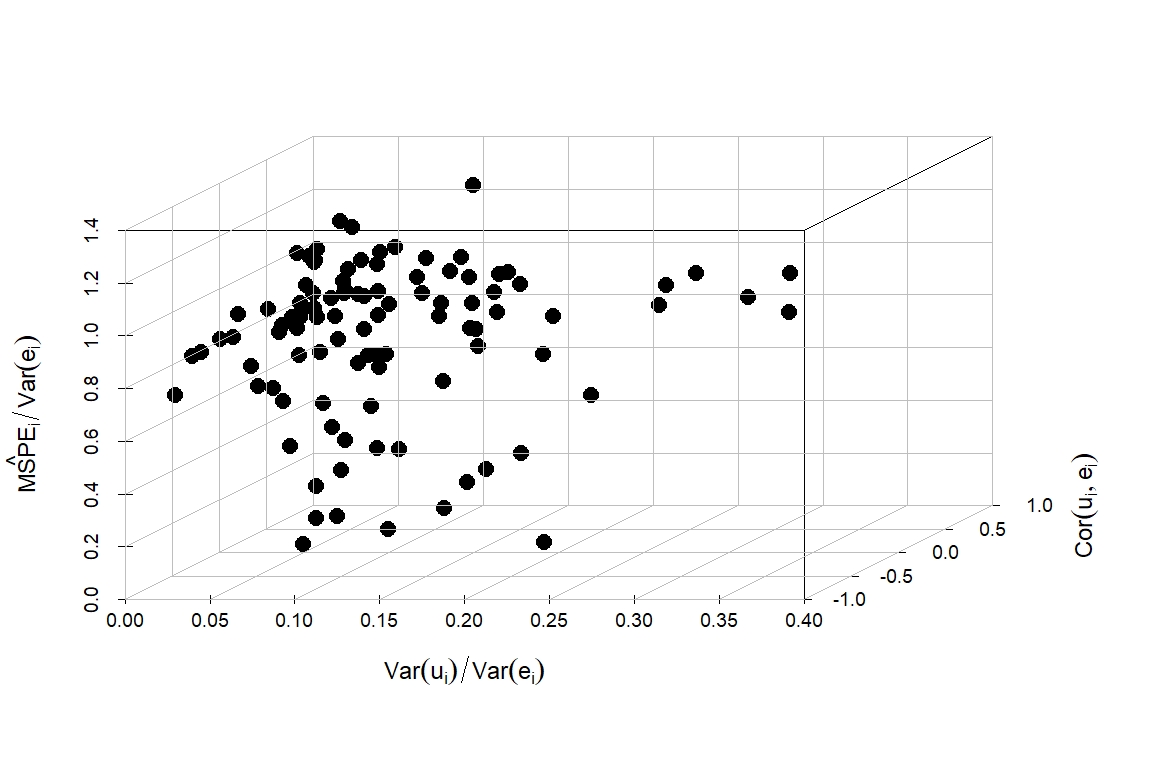
Figure 2 contains a scatterplot illuminating the relationship between the efficiency gain from prediction and the components of the design covariance matrix. The axis of the plot contains the ratios of the estimates of to the estimates of . The axis depicts the estimates of . The axis has the relative mean square prediction error, defined as the ratio of the estimated MSPE of the predictor to the estimated sampling variance of the direct estimator. A ratio below one means that the predictor is more efficient than the direct estimator.
From Figure 2, it is apparent that an efficiency gain is attained for most counties. The relative mean square prediction errors range from 0.056 to 1.222, and the average is 0.781. The efficiency gains are often pronounced when and are both small. For counties where the estimated MSPE of the predictor exceeds the estimated variance of the direct estimator, tends to be relatively high. For instance, for the county with a relative mean square error of 1.222, . This mirrors the simulation results for the configuration with small measurement error variance and high correlation. Overall, the estimated efficiency gains from small area modeling are substantial.
The left panel of Figure 3 contains a scatterplot of the predictors on the vertical axis against the direct estimators on the horizontal axis. The line in the plot is the 45-degree line through the origin. Small area prediction has the expected shrinkage effect. Prediction increases direct estimators that are unusually low and decreases direct estimators that are unusually high.
The right panel of Figure 3 contains a plot of the square roots of the mean square prediction errors against the standard errors of the direct estimators. The line is again the 45-degree line through the origin. For most counties, prediction renders an efficiency gain relative to the direct estimator. The reduction in MSPE from prediction is often substantial. When the MSPE exceeds the estimated variance of the direct estimator, the estimated loss of efficiency is minimal.

Discussion
We conduct an extensive study of the properties of a small area predictor that recognizes a correlation between the measurement error in the covariate and the sampling error in the response. The simulation studies illustrate the dangers of naively applying the Fay-Herriot predictor when the covariate and response are estimators from the same survey. The Fay-Herriot predictor can be less efficient than the direct estimator, and the corresponding MSPE estimator can have a severe negative bias for the MSPE of the predictor. The problems with the Fay-Herriot predictor persist even when for all .
The proposed predictor rectifies the problems with the Fay-Herriot predictor and is more efficient than other alternatives considered in the simulations. In both the simulations and the data analysis, the efficiency of the proposed method relative to the direct estimator depends on the nature of . In the CEAP study, runoff varies less within a county than does sheet and rill erosion, and substantial gains in efficiency from small area prediction are observed for most counties. Without the methodology presented in this paper, the use of runoff as a covariate would be impossible. Our methodology is of general interest beyond the CEAP study. We provide a theoretically sound estimation procedure for use in conjunction with the simple practice of using estimators from related surveys as covariates and response variables. The methodology has potential use in a wide range of applications in the area of official statistics.
References
- Arima et al. (2017) Arima, S., Bell, W. R., Datta, G. S., Franco, C. and Liseo, B. (2017) Multivariate Fay–Herriot Bayesian estimation of small area means under functional measurement error Journal of the Royal Statistical Society: Series A (Statistics in Society) 180, 1191–1209 DOI: 10.1111/rssa.12321.
- Arima et al. (2012) Arima, S., Datta, G. S. and Liseo, B. (2012) Objective Bayesian analysis of a measurement error small area model Bayesian Analysis 7, 363 – 384 DOI: 10.1214/12-BA712.
- Arima et al. (2015) Arima, S., Datta, G. S. and Liseo, B. (2015) Bayesian estimators for small area models when auxiliary information is measured with error Scandinavian Journal of Statistics 42, 518–529 DOI: 10.1111/sjos.12120.
- Bell et al. (2019) Bell, W. R., Chung, H. C., Datta, G. S. and Franco, C. (2019) Measurement error in small area estimation: Functional versus structural versus naive models Survey Methodology 45, 61–80.
- Berg and Chandra (2014) Berg, E. and Chandra, H. (2014) Small area prediction for a unit-level lognormal model Computational Statistics & Data Analysis 78, 159–175 DOI: 10.1016/j.csda.2014.03.007.
- Berg and Lee (2019) Berg, E. and Lee, D. (2019) Prediction of small area quantiles for the conservation effects assessment project using a mixed effects quantile regression model Annals of Applied Statistics 13, 2158–2188 DOI: 10.1214/19-AOAS1276.
- Berg and Yu (2019) Berg, E. and Yu, C. (2019) Semiparametric quantile regression imputation for a complex survey with application to the conservation effects assessment project Survey methodology DOI: 10.1214/12-BA712.
- Burgard et al. (2020) Burgard, J. P., Esteban, M. D., Morales, D. and Pérez, A. (2020) A Fay–Herriot model when auxiliary variables are measured with error Test 29, 166–195 DOI: 10.1007/s11749-019-00649-3.
- Burgard et al. (2021) Burgard, J. P., Esteban, M. D., Morales, D. and Pérez, A. (2021) Small area estimation under a measurement error bivariate Fay–Herriot model Statistical Methods & Applications 30, 79–108 DOI: 10.1007/s10260-020-00515-9.
- Burgard et al. (2022) Burgard, J. P., Krause, J. and Morales, D. (2022) A measurement error Rao–Yu model for regional prevalence estimation over time using uncertain data obtained from dependent survey estimates TEST 31, 204–234 DOI: 10.1111/rssa.12321.
- Carroll et al. (2006) Carroll, R. J., Ruppert, D., Stefanski, L. A. and Crainiceanu, C. M. (2006) Measurement error in nonlinear models: a modern perspective Chapman and Hall/CRC press, New York DOI: 10.1201/9781420010138.
- Datta et al. (2010) Datta, G. S., Rao, J. and Torabi, M. (2010) Pseudo-empirical Bayes estimation of small area means under a nested error linear regression model with functional measurement errors Journal of Statistical Planning and Inference 140, 2952–2962 DOI: 10.1016/j.jspi.2010.03.046.
- Erciulescu and Fuller (2016) Erciulescu, A. L. and Fuller, W. A. (2016) Small area prediction under alternative model specifications Statistics in Transition new series 17, 9–24 DOI: 10.21307/stattrans-2016-003.
- Fay and Herriot (1979) Fay, R. E. and Herriot, R. A. (1979) Estimates of income for small places: an application of James-Stein procedures to census data Journal of the American Statistical Association 74, 269–277 DOI: 10.1080/01621459.1979.10482505.
- Franco and Bell (2022) Franco, C. and Bell, W. R. (2022) Using American Community Survey data to improve estimates from smaller us surveys through bivariate small area estimation models Journal of Survey Statistics and Methodology 10, 225–247 DOI: 10.1093/jssam/smaa040.
- Fuller (2009) Fuller, W. A. (2009) Measurement error models vol. 305 John Wiley & Sons DOI: 10.1002/9780470316665.
- Ghosh and Sinha (2007) Ghosh, M. and Sinha, K. (2007) Empirical Bayes estimation in finite population sampling under functional measurement error models Journal of Statistical Planning and Inference 137, 2759–2773 DOI: 10.1016/j.jspi.2006.08.008.
- Ghosh et al. (2006) Ghosh, M., Sinha, K. and Kim, D. (2006) Empirical and hierarchical Bayesian estimation in finite population sampling under structural measurement error models Scandinavian Journal of Statistics 33, 591–608 DOI: 10.1111/j.1467-9469.2006.00492.x.
- Jiang and Lahiri (2006) Jiang, J. and Lahiri, P. (2006) Mixed model prediction and small area estimation Test 15, 1–96 DOI: 10.1007/BF02595419.
- Kim et al. (2015) Kim, J. K., Park, S. and Kim, S.-Y. (2015) Small area estimation combining information from several sources Survey Methodology 41, 21–36.
- Li and Lahiri (2010) Li, H. and Lahiri, P. (2010) An adjusted maximum likelihood method for solving small area estimation problems Journal of Multivariate Analysis 101, 882–892 DOI: 10.1016/j.jmva.2009.10.009.
- Lyu et al. (2020) Lyu, X., Berg, E. J. and Hofmann, H. (2020) Empirical Bayes small area prediction under a zero-inflated lognormal model with correlated random area effects Biometrical Journal 62, 1859–1878 DOI: 10.1002/bimj.202000029.
- Mosaferi et al. (2021) Mosaferi, S., Ghosh, M. and Steorts, R. C. (2021) Transformed Fay-Herriot model with measurement error in covariates Communications in Statistics-Simulation and Computation 1–18 DOI: 10.1080/03610918.2021.1901917.
- Pfeffermann (2013) Pfeffermann, D. (2013) New important developments in small area estimation Statistical Science 28, 40–68 DOI: 10.1214/12-STS395.
- Rao and Molina (2015) Rao, J. and Molina, I. (2015) Small area estimation second edition Hoboken, New Jersey DOI: 10.1002/9781118735855.fmatter.
- Shao (2003) Shao, J. (2003) Mathematical statistics Springer Science & Business Media, New York, NY DOI: 10.1007/0-387-28276-9.
- Torabi (2011) Torabi, M. (2011) Small area estimation using survey weights with functional measurement error in the covariate Australian & New Zealand Journal of Statistics 53, 141–155 DOI: 10.1111/j.1467-842X.2011.00623.x.
- Torabi (2012) Torabi, M. (2012) Small area estimation using survey weights under a nested error linear regression model with structural measurement error Journal of Multivariate Analysis 109, 52–60 DOI: 10.1016/j.jmva.2012.02.015.
- Torabi et al. (2009) Torabi, M., Datta, G. S. and Rao, J. (2009) Empirical Bayes estimation of small area means under a nested error linear regression model with measurement errors in the covariates Scandinavian Journal of Statistics 36, 355–369 DOI: 10.1111/j.1467-9469.2008.00623.x.
- Ybarra (2003) Ybarra, L. (2003) Small Area Estimation using Data from Multiple Surveys Ph.D. thesis Arizona State University.
- Ybarra and Lohr (2008) Ybarra, L. M. and Lohr, S. L. (2008) Small area estimation when auxiliary information is measured with error Biometrika 95, 919–931 DOI: 10.1093/biomet/asn048.
Appendix A: Derivation of Conditional Distribution of given
We provide further detail on the derivation of the distribution of given . Under the assumptions of the model (1), the bivariate distribution of can be stated as
where we have used the definition of as . By standard properties of the bivariate normal distribution,
and
Appendix B: Statistical Properties of Estimators and Predictors
We state and prove Theorems 1 and 2 for the case of univariate . For the univariate case, we parametrize as
We denote the univariate slope and estimator of as and , respectively.
Theorem 1: Assume the following assumptions hold:
- A.1
, where .
- A.2
, where .
- A.3
, where .
- A.4
=
, where for . - A.5
.
Then, .
Proof: One can express as , where is the univariate version of the vector defined in Section 2.2. Let denote the probability limit of for . By the law of large numbers and assumptions A.1-A.4, is finite. By assumption A.5, is a continuous function on a closed set containing , . The result then follows from the continuous mapping theorem. We present a more rigorous proof in the supplementary material.
Theorem 2: Let and let . Define
where . Assume that for any in the parameter space for ,
Then .
Proof: See the supplementary material.
Appendix C: Direct Estimators for CEAP
We explain how we estimate for the CEAP data. We let denote the index set for the elements in the sample for county . As in Berg and Yu 2019, we approximate the CEAP sample for a county as a Poisson sample. The inclusion probability for unit in county , denoted , is defined in Berg and Yu 2019. In CEAP operations, replication variance estimation procedures are used. We do not have access to the replicate weights for this analysis. The Poisson approximation preserves the calculated inclusion probabilities and enables a simple variance estimation procedure that is adequate for the purpose of this study.
We let and , respectively, denote the values for RUSLE2 and runoff for element in county . Then, we define , where . We define an estimate of the within-county variance for county by
where . By the delta method, an estimator of the sampling variance of is then
Supplement to “An application of a small area procedure with correlation between measurement error and sampling error to the Conservation Effects Assessment Project”
In this supplement, we prove Theorems 1-3 of the main document and present extended simulation results. The proofs are given in Section 1. The simulation output is provided in Sections 2-3.
Proofs
Proof of Theorem 1
The proof of Theorem 1 relies heavily on Theorem 1.14 (ii) of Shao 2003. For ease of reference for the reader, we state Theorem 1.14 (ii) of Shao 2003 as Lemma 1 below:
Lemma 1 (Theorem 1.14 (ii) of Shao 2003 ): Let be independent random variables with finite expectations. If there is a constant such that
then
Proof of Theorem 1: We now prove that . As notation, we let be the univariate version of the vector defined in Section 2.2 of the main document for . Then, , , , and . We first show that . Define . Then,
where , , and .
By A.1, . The are independent and . By normality, .
By A.3, . Lemma 1 with implies that . The are independent, , and
By A.4 and lemma 1 with , . The continuous mapping theorem then implies that . Similarly, let . Then,
By A.1, . By A.4 and lemma 1 with , . By normality, . Then, A.4 and lemma 1 imply that . The continuous mapping theorem then implies that
Similar arguments imply that
and
We have now established that
and
We can express the function defining as
where
and
Consider the function defined as . By A.5, . Now,
and
This verifies that
and
By A.5, and are continuous in a closed set containing . The continuous mapping theorem then implies that
and
This completes the proof of Theorem 1.
Proof of Theorem 2
Let be the root of the score equation such that
Note that is the maximum likelihood estimator that would be obtained if and were known. By standard maximum likelihood theory, . We expand the objective function defining around . A Taylor approximation gives
where is on the line segment between and , and is on the line segment between and .
We only require a first order approximation because we have already proved the consistency of in Theorem 1. We use the notation to denote the partial derivative of with respect to , evaluated at . Similarly, denotes the partial derivative of with respect to evaluated at .
Then, by the conditions in the statement of Theorem 2,
| (12) |
where
and
The right side of (12) is by Theorem 2. Then, , and . This completes the proof of Theorem 2.
Extended Simulation Results
Random components are multiples of distributions
We generate the random effects as , where , and we generate as , where and are independently distributed as random variables. Tables S.1 and S.2 present the results. For this simulation model, the random terms do not have finite fourth moments. Nonetheless, the properties of the proposed predictors and MSPE estimators mostly remain stable. The proposed estimators of regression coefficients are nearly unbiased. The heavy tails of the distribution exacerbate the bias of the estimator of . The bias for the estimator of has minimal impacts on the properties of the predictors and MSPE estimators. The proposed predictors are more efficient than the alternatives. The proposed MSPE estimator is a reasonable approximation for the MSPE of the predictor.
Random components are multiples of distributions
We generate the random effects as , where . Similarly, we generate as , where and have independent distributions, centered and scaled to have mean zero and unit variance. Tables S.3 and S.4 present the results. For this simulation model, the random effects have skewed distributions. Despite the skewness, the estimators of fixed parameters and predictors have reasonable properties. The estimators of regression coefficients are nearly unbiased. The estimator of can have a positive bias when and . Increasing the sample size to 500 reduces the magnitude of the bias substantially. Despite the bias for the estimator of , the proposed predictors are more efficient than the alternatives, and the proposed MSPE estimator is a reasonable approximation for the MSPE of the predictor.
| MC MSPE of Predictor | MC Mean Est. MSPE | ||||||||
|---|---|---|---|---|---|---|---|---|---|
| Direct | ME-Cor | YL | FH | ME-Cor-MSPE | FH-MSPE | ||||
| (0.250, 0.750, 0.200) | 100 | 0.939 | 0.705 | 0.707 | 0.804 | 0.749 | 0.447 | ||
| 500 | 0.988 | 0.731 | 0.741 | 0.805 | 0.740 | 0.461 | |||
| (0.250, 0.750, 0.800) | 100 | 1.015 | 1.012 | 1.116 | 1.543 | 1.001 | 0.096 | ||
| 500 | 0.977 | 0.972 | 1.084 | 1.555 | 1.001 | 0.051 | |||
| (0.750, 0.250, 0.200) | 100 | 0.320 | 0.318 | 0.325 | 0.340 | 0.334 | 0.297 | ||
| 500 | 0.333 | 0.330 | 0.339 | 0.352 | 0.334 | 0.298 | |||
| (0.750, 0.250, 0.800) | 100 | 0.334 | 0.222 | 0.431 | 0.569 | 0.223 | 0.279 | ||
| 500 | 0.330 | 0.215 | 0.431 | 0.559 | 0.218 | 0.281 | |||
| ME-Cor | YL | FH | ||||||||
|---|---|---|---|---|---|---|---|---|---|---|
| MC Mean | MC SD | MC Mean | MC SD | MC Mean | MC SD | |||||
| 100 | 0.999 | 0.314 | 0.976 | 0.277 | 1.206 | 0.280 | ||||
| 0.250 | 0.750 | 0.200 | 100 | 2.003 | 0.054 | 2.007 | 0.048 | 1.962 | 0.048 | |
| 100 | 0.402 | 1.697 | 0.252 | 1.765 | 1.022 | 1.789 | ||||
| 500 | 0.984 | 0.186 | 0.949 | 0.169 | 1.233 | 0.168 | ||||
| 0.250 | 0.750 | 0.200 | 500 | 2.003 | 0.034 | 2.010 | 0.030 | 1.954 | 0.030 | |
| 500 | 0.348 | 0.569 | 0.135 | 0.549 | 1.012 | 0.608 | ||||
| 100 | 1.000 | 0.241 | 0.811 | 0.236 | 1.082 | 0.227 | ||||
| 0.250 | 0.750 | 0.800 | 100 | 2.000 | 0.046 | 2.039 | 0.044 | 1.983 | 0.042 | |
| 100 | 0.355 | 0.592 | 0.036 | 0.465 | 0.114 | 0.525 | ||||
| 500 | 0.998 | 0.105 | 0.804 | 0.097 | 1.086 | 0.093 | ||||
| 0.250 | 0.750 | 0.800 | 500 | 2.000 | 0.020 | 2.041 | 0.018 | 1.982 | 0.017 | |
| 500 | 0.361 | 0.548 | 0.020 | 0.441 | 0.078 | 0.538 | ||||
| 100 | 0.898 | 0.570 | 0.897 | 0.508 | 1.810 | 0.456 | ||||
| 0.750 | 0.250 | 0.200 | 100 | 2.024 | 0.117 | 2.021 | 0.100 | 1.824 | 0.092 | |
| 100 | 0.505 | 1.101 | 0.450 | 1.184 | 3.225 | 1.388 | ||||
| 500 | 0.941 | 0.345 | 0.923 | 0.294 | 1.869 | 0.278 | ||||
| 0.750 | 0.250 | 0.200 | 500 | 2.012 | 0.070 | 2.016 | 0.060 | 1.819 | 0.056 | |
| 500 | 0.385 | 0.780 | 0.265 | 0.834 | 3.317 | 0.899 | ||||
| 100 | 0.959 | 0.447 | 0.845 | 0.389 | 1.528 | 0.384 | ||||
| 0.750 | 0.250 | 0.800 | 100 | 2.007 | 0.080 | 2.031 | 0.070 | 1.898 | 0.068 | |
| 100 | 0.456 | 1.234 | 0.169 | 1.058 | 2.168 | 1.348 | ||||
| 500 | 0.966 | 0.325 | 0.791 | 0.304 | 1.696 | 0.270 | ||||
| 0.750 | 0.250 | 0.800 | 500 | 2.007 | 0.066 | 2.045 | 0.063 | 1.854 | 0.054 | |
| 500 | 0.384 | 0.817 | 0.069 | 0.622 | 2.127 | 0.809 | ||||
| ME-Cor | YL | FH | ||||||||
|---|---|---|---|---|---|---|---|---|---|---|
| MC Mean | MC SD | MC Mean | MC SD | MC Mean | MC SD | |||||
| 100 | 1.002 | 0.287 | 0.954 | 0.273 | 1.243 | 0.264 | ||||
| 0.250 | 0.750 | 0.200 | 100 | 2.000 | 0.046 | 2.007 | 0.042 | 1.958 | 0.041 | |
| 100 | 0.347 | 0.298 | 0.123 | 0.259 | 1.043 | 0.382 | ||||
| 500 | 0.993 | 0.129 | 0.946 | 0.120 | 1.254 | 0.116 | ||||
| 0.250 | 0.750 | 0.200 | 500 | 2.000 | 0.025 | 2.011 | 0.023 | 1.946 | 0.022 | |
| 500 | 0.358 | 0.146 | 0.043 | 0.091 | 1.044 | 0.170 | ||||
| 100 | 1.002 | 0.164 | 0.857 | 0.167 | 1.063 | 0.161 | ||||
| 0.250 | 0.750 | 0.800 | 100 | 2.000 | 0.028 | 2.027 | 0.027 | 1.988 | 0.026 | |
| 100 | 0.351 | 0.145 | 0.000 | 0.000 | 0.071 | 0.101 | ||||
| 500 | 0.998 | 0.071 | 0.846 | 0.072 | 1.066 | 0.070 | ||||
| 0.250 | 0.750 | 0.800 | 500 | 2.000 | 0.012 | 2.029 | 0.012 | 1.987 | 0.011 | |
| 500 | 0.355 | 0.065 | 0.000 | 0.000 | 0.045 | 0.048 | ||||
| 100 | 0.960 | 0.462 | 0.912 | 0.400 | 2.022 | 0.332 | ||||
| 0.750 | 0.250 | 0.200 | 100 | 2.010 | 0.112 | 2.021 | 0.099 | 1.782 | 0.082 | |
| 100 | 0.457 | 0.573 | 0.332 | 0.635 | 3.382 | 0.823 | ||||
| 500 | 0.999 | 0.171 | 0.952 | 0.152 | 1.857 | 0.134 | ||||
| 0.750 | 0.250 | 0.200 | 500 | 2.001 | 0.038 | 2.010 | 0.033 | 1.827 | 0.029 | |
| 500 | 0.368 | 0.287 | 0.138 | 0.260 | 3.471 | 0.406 | ||||
| 100 | 0.994 | 0.320 | 0.830 | 0.290 | 1.630 | 0.258 | ||||
| 0.750 | 0.250 | 0.800 | 100 | 2.000 | 0.064 | 2.032 | 0.058 | 1.879 | 0.051 | |
| 100 | 0.414 | 0.442 | 0.025 | 0.184 | 2.272 | 0.637 | ||||
| 500 | 0.997 | 0.135 | 0.848 | 0.123 | 1.603 | 0.111 | ||||
| 0.750 | 0.250 | 0.800 | 500 | 2.001 | 0.027 | 2.029 | 0.023 | 1.884 | 0.022 | |
| 500 | 0.354 | 0.194 | 0.000 | 0.008 | 2.236 | 0.264 | ||||
| MC MSPE of Predictor | MC Mean Est. MSPE | ||||||||
|---|---|---|---|---|---|---|---|---|---|
| Direct | ME-Cor | YL | FH | ME-Cor-MSPE | FH-MSPE | ||||
| (0.250, 0.750, 0.200) | 100 | 1.012 | 0.755 | 0.764 | 0.828 | 0.743 | 0.492 | ||
| 500 | 1.007 | 0.743 | 0.759 | 0.807 | 0.740 | 0.485 | |||
| (0.250, 0.750, 0.800) | 100 | 1.016 | 1.009 | 1.116 | 1.589 | 1.001 | 0.094 | ||
| 500 | 1.006 | 0.999 | 1.108 | 1.615 | 1.001 | 0.048 | |||
| (0.750, 0.250, 0.200) | 100 | 0.336 | 0.334 | 0.343 | 0.355 | 0.334 | 0.301 | ||
| 500 | 0.335 | 0.333 | 0.344 | 0.355 | 0.333 | 0.301 | |||
| (0.750, 0.250, 0.800) | 100 | 0.337 | 0.215 | 0.444 | 0.563 | 0.218 | 0.286 | ||
| 500 | 0.336 | 0.213 | 0.444 | 0.565 | 0.212 | 0.285 | |||
Bivariate covariate
We validate the procedure for a model with two covariates, both of which are subject to measurement error. The simulation model is defined by
where and the distribution of is defined below. Instead of observing and , we observe
where
and
for all . As the model has more parameters than the model with a univariate covariate, we set for this simulation.
We calculate the estimators of fixed parameters, predictors, and estimator of the MSPE according to the proposed procedures. The MC mean of the estimators of is . The MC mean of the estimator of is 0.349. The average MC MSPE of the predictors is 0.2479. The average of the estimated MSPE is 0.2478. This validates the properties of the proposed procedure for the case of a bivariate covariate.
Comparison to Burgard et al. 2022
We compare the proposed (ME-Cor) predictor to the predictor derived using the method of Burgard et al. 2022. As in Burgard et al. 2022, we use maximum likelihood to estimate the fixed model parameters. We denote the maximum likelihood estimators by . We define a predictor based on the method of Burgard et al. 2022 for a univariate version of the measurement error model. We define the predictor of Burgard et al. 2022 as
where
and . For the simulation configuration in Table S.5, the proposed predictor has smaller average MSE than the predictor of Burgard et al. 2022.
| Burgard | ME-Cor | ||
|---|---|---|---|
| (0.25, 0.75, 0.20) | 100 | 0.743 | 0.732 |
| (0.25, 0.75, 0.20) | 500 | 0.760 | 0.747 |
| (0.25, 0.75, 0.80) | 100 | 1.115 | 1.006 |
| (0.25, 0.75, 0.80) | 500 | 1.087 | 0.998 |
| (0.75, 0.25, 0.20) | 100 | 0.377 | 0.342 |
| (0.75, 0.25, 0.20) | 500 | 0.370 | 0.335 |
| (0.75, 0.25, 0.80) | 100 | 0.681 | 0.215 |
| (0.75, 0.25, 0.80) | 500 | 0.695 | 0.214 |