跳到论文正文
W Papers独立论文阅读器 arXiv:2110.10210 论文正文 计算阅读时间 · 0%
引用这篇论文根据当前论文元数据生成,正式投稿前建议核对。


License: CC BY 4.0
arXiv:2110.10210v1 [math.PR] 19 Oct 2021

Long Random Matrices and Tensor Unfolding

Gérard Ben Arous Thanks: benarous@cims.nyu.edu    Daniel Zhengyu Huang Thanks: dzhuang@caltech.edu Affiliation: California Institute of Technology, Pasadena, CA    Jiaoyang Huang Thanks: jh4427@nyu.edu
Abstract

In this paper, we consider the singular values and singular vectors of low rank perturbations of large rectangular random matrices, in the regime the matrix is “long”: we allow the number of rows (columns) to grow polynomially in the number of columns (rows). We prove there exists a critical signal-to-noise ratio (depending on the dimensions of the matrix), and the extreme singular values and singular vectors exhibit a BBP type phase transition. As a main application, we investigate the tensor unfolding algorithm for the asymmetric rank-one spiked tensor model, and obtain an exact threshold, which is independent of the procedure of tensor unfolding. If the signal-to-noise ratio is above the threshold, tensor unfolding detects the signals; otherwise, it fails to capture the signals.

1 Introduction

High order arrays, or tensors have been actively considered in neuroimaging analysis, topic modeling, signal processing and recommendation system [25, 19, 26, 36, 50, 58, 55, 18, 54]. Researchers have made tremendous efforts to innovate effective methods for the analysis of tensor data. The spiked tensor model, introduced in [51] by Richard and Montanari, captures a number of statistical estimation tasks in which we need to extract information from a noisy high-dimensional data tensor. We are given a tensor 𝑿∈(ℝn)⊗k\bm{X}\in({\mathbb{R}}^{n})^{\otimes k} in the following form

𝑿=β𝒗1⊗𝒗2⊗⋯⊗𝒗k+𝑾,\displaystyle\bm{X}=\beta{\bm{v}}_{1}\otimes{\bm{v}}_{2}\otimes\cdots\otimes{\bm{v}}_{k}+\bm{W},

where 𝑾\bm{W} is a noise tensor, β>0\beta>0 corresponds to the signal-to-noise ratio (SNR), and 𝒗1⊗𝒗2⊗⋯⊗𝒗k{\bm{v}}_{1}\otimes{\bm{v}}_{2}\otimes\cdots\otimes{\bm{v}}_{k} is a rank one unseen signal tensor to be recovered.

When k=2k=2, the spiked tensor model reduces to the spiked matrix model of the form “signal ++ noise”, which has been intensively studied in the past twenty years. It is now well-understood that the extreme eigenvalues of low rank perturbations of large random matrices undergo a so-called BBP phase transition [3] along with the change of signal-to-noise ratio, first discovered by Baik, Péché and the first author. There is an order one critical signal-to-noise ratio βc\beta_{\rm c}, such that below βc\beta_{\rm c}, it is information-theoretical impossible to detect the spikes [49, 46, 45], and above βc\beta_{\rm c}, it is possible to detect the spikes by Principal Component Analysis (PCA). A body of work has quantified the behavior of PCA in this setting [33, 3, 4, 47, 11, 2, 34, 12, 15, 43, 56, 14, 23, 38, 22]. We refer readers to the review article [35] by Johnstone and Paul, for more discussion and references to this and related lines of work.

For the spiked tensor model with k⩾3k\geqslant 3, the same as the spiked matrix model, there is an order one critical signal-to-noise ratio βk\beta_{k} (depending on the order kk), such that below βk\beta_{k}, it is information-theoretical impossible to detect the spikes, and above βk\beta_{k}, the maximum likelihood estimator is a distinguishing statistics [16, 17, 39, 48, 32]. In the matrix setting the maximum likelihood estimator is the top eigenvector, which can be computed in polynomial time by, e.g., power iteration. However, for order k⩾3k\geqslant 3 tensor, computing the maximum likelihood estimator is NP-hard in generic setting. In this setting, two “phase transitions” are often studied. There is the critical signal-to-noise ratio SNRs​t​a​t=βk{}_{stat}=\beta_{k}, below which it is statistically impossible to estimate the parameters. Although above the threshold SNRstat, it is possible to estimate the parameters in theory, there is no known efficient algorithm (polynomial time) to achieve recovery close to the statistical threshold SNRstat. Thus many algorithm development fields are interested in another critical threshold SNRc​o​m​p⩾{}_{comp}\geqslant{}SNRstat below which it is impossible for an efficient algorithm to achieve recovery. For the spiked tensor model with k⩾3k\geqslant 3, it is widely believed there exists a computational-to-statistical gaps SNRc​o​m​p−{}_{comp}-{}SNRs​t​a​t>0{}_{stat}>0. We refer readers to the article [5] by Bandeira, Perry and Wein, for more detailed discussion on this phenomenon.

In the work [51] of Richard and Montanari, the algorithmic aspects of the spiked tensor model have been studied. They showed that tensor power iteration and approximate message passing algorithm with random initialization recovers the signal provided β≳n(k−1)/2\beta\gtrsim n^{(k-1)/2}. Based on heuristic arguments, they predicted that the necessary and sufficient condition for power iteration and approximate message passing (AMP) algorithm to succeed is β≳n(k−2)/2\beta\gtrsim n^{(k-2)/2}. This threshold was proven in [39] for AMP by Lesieur, Miolane, Lelarge, Krzakala and Zdeborová, for power iteration by Yang, Cheng and the last two authurs [31]. The same threshold was also achieved by using gradient descent and Langevin dynamics as studied by Gheissari, Jagannath and the first author [7].

In [51], Richard and Montanari also proposed a method based on tensor unfolding, which unfolds the tensor 𝑿\bm{X} to an nq×nk−qn^{q}\times n^{k-q} matrix 𝖬𝖺𝗍⁡(𝑿)\mathsf{Mat}(\bm{X}) for some 1⩽q⩽k−11\leqslant q\leqslant k-1,

𝖬𝖺𝗍⁡(𝑿)=β​𝒗​𝒖⊤+Z∈ℝnq×ℝnk−q.\displaystyle\mathsf{Mat}(\bm{X})=\beta{\bm{v}}{\bm{u}}^{\top}+Z\in{\mathbb{R}}^{n^{q}}\times{\mathbb{R}}^{n^{k-q}}. (1.1)

By taking q=⌊k/2⌋q=\lfloor{k/2}\rfloor and performing matrix PCA on 𝖬𝖺𝗍⁡(𝑿)\mathsf{Mat}(\bm{X}), they proved that the tensor unfolding algorithm reovers the signal provided β≳n(⌈k/2⌉−1)/2\beta\gtrsim n^{(\lceil k/2\rceil-1)/2}, and predicted that the necessary and sufficient condition for tensor unfolding is β≳n(k−2)/4\beta\gtrsim n^{(k-2)/4}.

Several other sophisticated algorithms for the spiked tensor model have been investigated in literature which achieves the sharp threshold β≳n(k−2)/4\beta\gtrsim n^{(k-2)/4}: Sum-of-Squares algorithms [29, 28, 37], sophisticated iteration algorithms [40, 57, 27], and an averaged version of gradient descent [13] by Biroli, Cammarota, Ricci-Tersenghi. The necessary part of this threshold still remains open. Its relation with hypergraphic planted clique problem was discussed in [41, 42] by Luo and Zhang. Its proven for k=3k=3 in [29] by Hopkins, Shi and Steurer, degree-44 sum-of-squares relaxations fail below this threshold. The candscape complexity of spiked tensor model was studied in [8] by Mei, Montanari, Nica and the first author. A new framework based on the Kac-Rice method that allows to compute the annealed complexity of the landscape has been proposed in [52] by Ros, Biroli,Cammarota and the first author, which was later used to analyze gradient-based algorithms in non-convex setting [53, 44] by Mannelli, Biroli, Cammarota, Krzakala, Urbani, and Zdeborová.

In this paper, we revisit the tensor unfolding algorithm introduced by Richard and Montanari. The unfolded matrix 𝖬𝖺𝗍⁡(𝑿)\mathsf{Mat}(\bm{X}) from (1.1) is a spiked matrix model in the form of “signal ++ noise”. However, it is different from spiked matrix models in random matrix literature, which requires the dimensions of the matrix to be comparable, namely the ratio of the number of rows and the number of columns converges to a fixed constant. In this setting, the singular values and singular vectors of the spiked matrix model (1.1) has been studied in [11] by Benaych-Georges and Nadakuditi.

For the unfolded matrix 𝖬𝖺𝗍⁡(𝑿)\mathsf{Mat}(\bm{X}), its dimensions are not comparable. As the size nn of the tensor goes to infinity, the ratio of the number of rows and columns goes to zero or infinity, unless q=k/2q=k/2 (in this case 𝖬𝖺𝗍⁡(𝑿)\mathsf{Mat}(\bm{X}) is a square matrix). In this paper, we study the singular values and singular vectors of the spiked matrix model (1.1) in the case where the number of rows (columns) grows polynomially in the number of columns (rows), which we call low rank perturbation of long random matrices. In the case when β=0\beta=0, the estimates of singular values and singular vectors for long random matrices follow from [1] by Alex, Erdős, Knowles, Yau, and Yin.

To study the low rank perturbations of long random matrices, we use the master equations from [11], which characterize the outliers of the perturbed random matrices, and the associated singular values. To analyze the master equations, we use the estimates of singular values and Green’s functions of long random matrices from [1]. Comparing with the setting that the ratio of the number of rows and the number of columns converges to a fixed constant, the challenge is to obtain uniform estimates for the errors in the master equations, which depends only on the number of rows. In this way, we can allow the number of columns to grow much faster than the number of rows. For the low rank perturbation of long random matrices, we prove there exists a critical signal-to-noise ratio βc\beta_{\rm c} (depending on the dimensions of the matrix), and it exhibit a BBP type phase transition. We also obtain estimates of the singular values and singular vectors for this model. Moreover, we also have precise estimates when the signal-to-noise ratio β\beta is close to the threshold βc\beta_{\rm c}. In particular, our results also apply when β\beta is close to βc\beta_{\rm c} in mesoscopic scales. In an independent work [24] by Feldman, this model has been studied under different assumptions. We refer to Section 2.2 for a more detailed discussion of the differences.

Our results for low rank perturbation of long random matrices can be used to study the unfolded matrix 𝖬𝖺𝗍⁡(𝑿)\mathsf{Mat}(\bm{X}). For the signal-to-noise ratio β=λ​n(k−2)/4\beta=\lambda n^{(k-2)/4} and any 1⩽q⩽k−11\leqslant q\leqslant k-1, if λ>1\lambda>1, the PCA on 𝖬𝖺𝗍⁡(𝑿)\mathsf{Mat}(\bm{X}) detects the signal tensor; if λ<1\lambda<1, the PCA on 𝖬𝖺𝗍⁡(𝑿)\mathsf{Mat}(\bm{X}) fails to capture the signal tensor. This matches the conjectured algorithmic threshold for the spiked tensor model from [51]. It is worth mentioning that the threshold we get is independent of the tensor unfolding procedure, namely, it is independent of the choice of qq. For q>1q>1, a further recursive unfolding is needed to recover individual signals 𝒗i{\bm{v}}_{i}, which increases the computational cost. We propose to simply take q=1q=1 in the tensor unfolding algorithm for each coordinate axis, and unfold the tensor to an n×nk−1n\times n^{k-1} matrix, which gives good approximation of individual signals 𝒗i{\bm{v}}_{i}, provided λ>1\lambda>1. In tensor literature, this algorithm is exactly the truncated higher order singular value decomposition (HOSVD) introduced in [20] by De Lathauwer, De Moor and Vandewalle. Later, they developed the higher order orthogonal iteration (HOOI) in [21], which uses the truncated HOSVD as initialization combining with a power iteration, to find the best low-multilinear-rank approximation of a tensor. The performance of HOOI was analyzed in [57] by Zhang and Xia, for the spiked tensor model. It was proven that for the signal-to-noise ratio β=λ​n(k−2)/4\beta=\lambda n^{(k-2)/4} satisfies λ⩾Cg​a​p\lambda\geqslant C_{gap} for some large constant Cg​a​p>0C_{gap}>0, HOOI converges within a logarithm factor of iterations.

The paper is organized as follows. In Section 2, we state the main results on the singular values and vectors of low rank perturbations of long random matrices. In Section 3 we study the spiked tensor model, as an application of our results on low rank perturbations of long random matrices. The proofs of our main results are given in Section 4.

Notations For two numbers X,YX,Y, we write that X=O⁡(Y)X=\OO(Y) if there exists a universal constant C>0C>0 such that |X|⩽C​Y|X|\leqslant CY. We write X=o⁡(Y)X=\oo(Y), or X≪YX\ll Y if the ratio |X|/Y→∞|X|/Y\rightarrow\infty as nn goes to infinity. We write X≍YX\asymp Y if there exists a universal constant C>0C>0 such that Y/C⩽|X|⩽C​YY/C\leqslant|X|\leqslant CY. We denote the index set [[k]]={1,2,⋯,k}[\![{k}]\!]=\{1,2,\cdots,k\}. We say an event Ω\Omega holds with high probability if for any large C>0C>0, ℙ⁡(Ω)⩾1−n−C\mathbb{P}(\Omega)\geqslant 1-n^{-C} for nn large enough. We write X≺YX\prec Y or X=O≺⁡(Y)X=\OO_{\prec}(Y), if XX is stochastically dominated by YY in the sense that for all large C>0C>0, we have

ℙ⁡(X⩾n1/C​Y)⩽n−C,\displaystyle\mathbb{P}(X\geqslant n^{1/C}Y)\leqslant n^{-C},

for large enough nn.

Acknowledgements The research of J.H. is supported by the Simons Foundation as a Junior Fellow at the Simons Society of Fellows, and NSF grant DMS-2054835.

2 Main Results

In this section, we state our main results on the singular values and singular vectors of low rank perturbations of long random matrices. Let Z∈ℝn×mZ\in{\mathbb{R}}^{n\times m} be an n×mn\times m random matrices, with i.i.d. random entries Zi​jZ_{ij} satisfying

Assumption 2.1.

The entries of ZZ are i.i.d., and have mean zero and variance 1/n1/n, and for any integer p⩾1p\geqslant 1,

𝔼⁡[Zi​j]=0,𝔼⁡[Zi​j2]=1n,𝔼⁡[Zi​j2​p]⩽Cpnp,1⩽i⩽n,1⩽j⩽m.\displaystyle\mathbb{E}[Z_{ij}]=0,\hskip 10.00002pt\mathbb{E}[Z_{ij}^{2}]=\frac{1}{n},\hskip 10.00002pt\mathbb{E}[Z_{ij}^{2p}]\leqslant\frac{C_{p}}{n^{p}},\hskip 10.00002pt1\leqslant i\leqslant n,\hskip 10.00002pt1\leqslant j\leqslant m.

We introduce the parameter ϕ:=m/n\phi:=\sqrt{m/n}. It is well-known that for m,n→∞m,n\rightarrow\infty, if their ratio converges to m/n=ϕ2→ϕ∗2∈[1,∞)m/n=\phi^{2}\rightarrow\phi_{*}^{2}\in[1,\infty) which is independent of nn, the empirical eigenvalue distribution of Z​Z⊤ZZ^{\top} converges to the Marchenko-Pastur law

(x−(ϕ∗−1)2)​((ϕ∗+1)2−x)2​π​x​d​x,\displaystyle\frac{\sqrt{\left(x-\left(\phi_{*}-1\right)^{2}\right)\left(\left(\phi_{*}+1\right)^{2}-x\right)}}{2\pi x}{\rm d}x, (2.1)

supported on [(ϕ∗−1)2,(ϕ∗+1)2][(\phi_{*}-1)^{2},(\phi_{*}+1)^{2}].

In this paper, we consider the case where the ratio m/n=ϕ2m/n=\phi^{2} depends on nn, satisfying that n1/C⩽ϕ⩽nCn^{1/C}\leqslant\phi\leqslant n^{C} for some constant C>0C>0. In Section 2.1, we collect some results on singular values of the long random matrix ZZ from [1]. Using the estimates of the singular values and singular vectors of long random matrices as input, we can study low rank perturbations of long random matrices. We consider rank one perturbation of long random matrices in the form,

β​𝒗​𝒖⊤+Z∈ℝn×m,\displaystyle\beta{\bm{v}}{\bm{u}}^{\top}+Z\in{\mathbb{R}}^{n\times m}, (2.2)

where 𝒗∈ℝn{\bm{v}}\in{\mathbb{R}}^{n}, 𝒖∈ℝm{\bm{u}}\in{\mathbb{R}}^{m} are unit vectors, and ZZ is an n×mn\times m random matrix satisfying Assumption 2.1. We state our main results on the singular values and singular vectors of low rank perturbations of long random matrices (2.2) in Section 2.2.

2.1 Singular values of Long Random Matrices

Let ZZ be an n×mn\times m random matrix, with entries satisfying Assumption 2.1. Let ϕ=m/n\phi=\sqrt{m/n} satisfy that n1/C⩽ϕ⩽nCn^{1/C}\leqslant\phi\leqslant n^{C} for some constant C>0C>0. The eigenvalues of sample covariance matrices Z​Z⊤ZZ^{\top} in this setting have been well studied in [1]. We denote the singular values of ZZ as

s1⩾s2⩾⋯⩾sn⩾0.\displaystyle s_{1}\geqslant s_{2}\geqslant\cdots\geqslant s_{n}\geqslant 0.

They are square roots of eigenvalues of the sample covariance matrices Z​Z⊤ZZ^{\top}. As an easy consequence of [1, Theorem 2.10], we have the following theorem on the estimates of the largest singular value of ZZ.

Theorem 2.2.

Under Assumption 2.1, let ϕ=m/n\phi=\sqrt{m/n} with n1/C⩽ϕ⩽nCn^{1/C}\leqslant\phi\leqslant n^{C}. Fix an arbitrarily small δ>0\delta>0, with high probability the largest singular value s1s_{1} of ZZ satisfies

|s1−(ϕ+1)|⩽nδn2/3,\displaystyle|s_{1}-(\phi+1)|\leqslant\frac{n^{\delta}}{n^{2/3}}, (2.3)

provided nn is large enough.

The results in [1] give estimates of each eigenvalues of the sample covariance matrix Z​Z⊤ZZ^{\top} away from 00, see Theorem 4.1. It also gives estimates of locations of each singular value of ZZ. In particular, it implies that the empirical singular value distribution ∑i=1nδsi/n\sum_{i=1}^{n}\delta_{s_{i}}/n of ZZ is close to the pushforward of the Marchenko-Pastur law (after proper normalization) by the map x↦xx\mapsto\sqrt{x},

ρϕ​(x)​d​x=(x2−(ϕ−1)2)​((ϕ+1)2−x2)π​x​d​x.\displaystyle\phantom{{}={}}\rho_{\phi}(x){\rm d}x=\frac{\sqrt{\left(x^{2}-\left(\phi-1\right)^{2}\right)\left(\left(\phi+1\right)^{2}-x^{2}\right)}}{\pi x}{\rm d}x.

We remark that ρϕ\rho_{\phi} depends on m,nm,n through ϕ\phi and is supported on [ϕ−1,ϕ+1][\phi-1,\phi+1]. As ϕ→∞\phi\rightarrow\infty with nn, ρϕ​(x)\rho_{\phi}(x) after shifting by ϕ\phi, i.e. ρϕ​(x+ϕ)\rho_{\phi}(x+\phi), converges to the semi-circle distribution on [−1,+1][-1,+1]:

ρϕ​(x+ϕ)​d​x→2​(x+1)​(1−x)π.\displaystyle\rho_{\phi}(x+\phi){\rm d}x\rightarrow\frac{2\sqrt{(x+1)(1-x)}}{\pi}.

See Figure 1 for some plots of ρϕ\rho_{\phi}. One can see that the extreme singular values stick to the boundary of the support of the limiting empirical measure.

Refer to caption
Figure 1: The empirical singular value distribution of ZZ, with n=1000n=1000 and m=n,n1.5,n2m=n,n^{1.5},n^{2}. When ϕ=m/n\phi=\sqrt{m/n} is large, the empirical singular value converges to the Semicircle distribution supported on [ϕ−1,ϕ+1][\phi-1,\phi+1].

2.2 Low Rank Perturbations of Long Random Matrices

Let ZZ be an n×mn\times m random matrix, with entries satisfying Assumption 2.1. Let ϕ=m/n\phi=\sqrt{m/n}. Without loss of generality we can assume that ϕ⩾1\phi\geqslant 1, otherwise, we can simply study the transpose of ZZ. We allow ϕ\phi to grow with nn at any polynomial rate, 1⩽ϕ⩽nC1\leqslant\phi\leqslant n^{C} for any large number C>0C>0. In this regime, ZZ is a long random matrix.

In this section, we state our main results on the rank one perturbation of long random matrices from (2.2):

β​𝒗​𝒖⊤+Z∈ℝn×m,\displaystyle\beta{\bm{v}}{\bm{u}}^{\top}+Z\in{\mathbb{R}}^{n\times m}, (2.4)

where 𝒗∈ℝn{\bm{v}}\in{\mathbb{R}}^{n}, 𝒖∈ℝm{\bm{u}}\in{\mathbb{R}}^{m} are unit vectors. As in Theorem 2.2, in this setting, the singular values of ZZ are roughly supported on the interval [ϕ−1,ϕ+1][\phi-1,\phi+1]. The following theorem states that there is an exact nn-dependent threshold ϕ\sqrt{\phi}, if β\beta is above the threshold, β​𝒗​𝒖⊤+Z\beta{\bm{v}}{\bm{u}}^{\top}+Z has an outlier singular value; if β\beta is below this threshold, there are no outlier singular values, and all the singular values are stick to the bulk.

Theorem 2.3.

We assume Assumption 2.1 and 1⩽ϕ=m/n⩽nC1\leqslant\phi=\sqrt{m/n}\leqslant n^{C}. Let β=λ​ϕ\beta=\lambda\sqrt{\phi} with λ⩾0\lambda\geqslant 0, fix arbitrarily small 𝔠>0{\mathfrak{c}}>0, and denote s^1\hat{s}_{1} the largest singular value of β​𝐯​𝐮⊤+Z\beta{\bm{v}}{\bm{u}}^{\top}+Z. For any small δ>0\delta>0, if λ⩾1+n−1/3+𝔠\lambda\geqslant 1+n^{-1/3+{\mathfrak{c}}}, with high probability, the largest singular value s^1\hat{s}_{1} of β​𝐯​𝐮⊤+Z\beta{\bm{v}}{\bm{u}}^{\top}+Z is an outlier, and explicitly given by

s^1=ϕ2+(λ2+1/λ2)​ϕ+1+O⁡(nδ​(λ−1)1/2n1/2​ϕ).\displaystyle\hat{s}_{1}=\sqrt{\phi^{2}+(\lambda^{2}+1/\lambda^{2})\phi+1}+\OO\left(\frac{n^{\delta}(\lambda-1)^{1/2}}{n^{1/2}\phi}\right). (2.5)

If λ⩽1+n−1/3+𝔠\lambda\leqslant 1+n^{-1/3+{\mathfrak{c}}}, with high probability, β​𝐯​𝐮⊤+Z\beta{\bm{v}}{\bm{u}}^{\top}+Z does not have outlier singular values, and the largest singular value s^1\hat{s}_{1} satisfies

s^1⩽ϕ+1+n−2/3+3𝔠,\displaystyle\hat{s}_{1}\leqslant\phi+1+n^{-2/3+3{\mathfrak{c}}}, (2.6)

provided nn is large enough.

We refer to Figure 2 for an illustration of Theorem 2.3. Theorem 2.3 also characterizes the behavior of the outlier in the critical case, when λ\lambda is close to 11.

Refer to caption
Figure 2: The empirical singular value distribution of β​𝒗​𝒖⊤+Z\beta{\bm{v}}{\bm{u}}^{\top}+Z, with n=1000n=1000,m=n1.5m=n^{1.5}, and β=λ​(m/n)1/4\beta=\lambda(m/n)^{1/4} for λ=1,1.5,2\lambda=1,1.5,2. We marked the predicted outlier by ×\times as given by formula (2.5).

We have similar transition for the singular vectors. If β\beta is above the threshold ϕ\sqrt{\phi}, the left singular vector 𝒗^1\hat{\bm{v}}_{1} associated with the largest singular value of β​𝒗​𝒖⊤+Z\beta{\bm{v}}{\bm{u}}^{\top}+Z has a large component in the signal 𝒗{\bm{v}} direction; If β\beta is below the threshold ϕ\sqrt{\phi}, the projection of 𝒗^1\hat{\bm{v}}_{1} on the signal 𝒗{\bm{v}} direction vanishes.

Theorem 2.4.

We assume Assumption 2.1 and 1⩽ϕ=m/n⩽nC1\leqslant\phi=\sqrt{m/n}\leqslant n^{C}. Let β=λ​ϕ\beta=\lambda\sqrt{\phi} with λ⩾0\lambda\geqslant 0, fix arbitrarily small 𝔠>0{\mathfrak{c}}>0, and denote s^1\hat{s}_{1} the largest singular value of β​𝐯​𝐮⊤+Z\beta{\bm{v}}{\bm{u}}^{\top}+Z. For any small δ>0\delta>0, if λ⩾1+n−1/3+𝔠\lambda\geqslant 1+n^{-1/3+{\mathfrak{c}}}, with high probability, the left singular vector 𝐯^1\hat{\bm{v}}_{1} associated with the largest singular value of β​𝐯​𝐮⊤+Z\beta{\bm{v}}{\bm{u}}^{\top}+Z has a large component in the signal 𝐯{\bm{v}} direction:

|⟨𝒗^1,𝒗⟩|=(1+O⁡(nδn1/2​(λ−1)3/2))​(λ4−1)λ4+λ2/ϕ.\displaystyle|\langle\hat{\bm{v}}_{1},{\bm{v}}\rangle|=\left(1+\OO\left(\frac{n^{\delta}}{n^{1/2}(\lambda-1)^{3/2}}\right)\right)\sqrt{\frac{(\lambda^{4}-1)}{\lambda^{4}+\lambda^{2}/\phi}}. (2.7)

And similar estimates for the right singular vector 𝐮^1\hat{\bm{u}}_{1} associated with the largest singular value of β​𝐯​𝐮⊤+Z\beta{\bm{v}}{\bm{u}}^{\top}+Z

|⟨𝒖^1,𝒖⟩|=(1+O≺⁡(1n1/2​(λ−1)3/2))​λ4−1λ2​(λ2+ϕ).\displaystyle|\langle\hat{{\bm{u}}}_{1},{\bm{u}}\rangle|=\left(1+\OO_{\prec}\left(\frac{1}{n^{1/2}(\lambda-1)^{3/2}}\right)\right)\sqrt{\frac{\lambda^{4}-1}{\lambda^{2}(\lambda^{2}+\phi)}}. (2.8)

If λ⩽1+n−1/3+𝔠\lambda\leqslant 1+n^{-1/3+{\mathfrak{c}}}, with high probability, the projection of 𝐯^1\hat{\bm{v}}_{1} on 𝐯{\bm{v}}, and the projection of 𝐮^1\hat{\bm{u}}_{1} on 𝐮{\bm{u}} are upper bounded by

max{|⟨𝒗^1,𝒗⟩|,|⟨𝒖^1,𝒖⟩|}⩽n4​𝔠min{n−1/6,1n​(λ−1)},\displaystyle\max\{|\langle\hat{\bm{v}}_{1},{\bm{v}}\rangle|,|\langle\hat{\bm{u}}_{1},{\bm{u}}\rangle|\}\leqslant n^{4{\mathfrak{c}}}\min\left\{n^{-1/6},\frac{1}{\sqrt{n}(\lambda-1)}\right\}, (2.9)

provided nn is large enough.

Remark 2.5.

We remark that when the ratio ϕ=m/n\phi=\sqrt{m/n} goes to infinity with nn, with λ\lambda fixed, then from (2.7), |⟨𝐯^1,𝐯⟩||\langle\hat{\bm{v}}_{1},{\bm{v}}\rangle| converges to 1−λ−4\sqrt{1-\lambda^{-4}}, and from (2.8), |⟨𝐮^1,𝐮⟩||\langle\hat{\bm{u}}_{1},{\bm{u}}\rangle| converges to 00.

Remark 2.6.

In this paper, for simplicity of notations, we only consider rank one perturbations of long random matrices. Our method can as well be used to study any finite rank perturbations of long random matrices.

The singular values and vectors of low rank perturbations of large rectangular random matrices has previously been studied in [11] by Benaych-Georges and Nadakuditi. Our main results Theorems 2.3 and 2.4 are generalization of their results in two directions. Firstly, in [11], the ratio ϕ=m/n\phi=\sqrt{m/n} is assumed to converge to a constant independent of nn. In our setting, we allow ϕ\phi to have polynomial growth in nn. As we will see in Section 3, this will be crucial for us to study the tensor principle component analysis. Secondly, we allow the signal-to-noise ratio to be close to the threshold (depending on nn), and our main results characterize the behaviors of singular values and singular vectors in this regime. In an independent work [24] by Feldman, the singular values and vectors of multi-rank perturbations of long random matrices have been studied under the assumption that either the signal vectors contains i.i.d. entries with mean zero and variance one, or the noise matrix has Gaussian entries. Both proofs use the master equations which characterize the singular values and singular vectors of low rank perturbations of rectangular random matrices developed in [11], see Section 4.2. To analyze the master equation, in [24], Feldman needs that the signal vectors have i.i.d. entries with mean zero and variance one. Our argument uses results from [1], which gives Green’s function estimates of long random matrices, and works for any (deterministic) signal vectors.

3 Tensor PCA

As an application of our main results Theorems 2.3 and 2.4, in this section, we use them to study the asymmetric rank-one spiked tensor model as introduced in [51]:

𝑿=β𝒗1⊗𝒗2⊗⋯⊗𝒗k+𝑾,\displaystyle\bm{X}=\beta{\bm{v}}_{1}\otimes{\bm{v}}_{2}\otimes\cdots\otimes{\bm{v}}_{k}+\bm{W}, (3.1)

where

  • •

    𝑿∈⊗kℝn\bm{X}\in\otimes^{k}{\mathbb{R}}^{n} is the kk-th order tensor observation.

  • •

    𝑾∈⊗kℝn\bm{W}\in\otimes^{k}{\mathbb{R}}^{n} is a noise tensor. The entries of 𝑾\bm{W} are independent random variables with mean zero and variance 1/n1/n.

  • •

    β∈ℝ\beta\in{\mathbb{R}} is the signal-to-noise ratio.

  • •

    𝒗i∈ℝn{\bm{v}}_{i}\in{\mathbb{R}}^{n} are unknown unit vectors to be recovered.

The goal is to perform reliable estimation and inference on the unseen signal tensor 𝒗1⊗𝒗2⊗⋯⊗𝒗k{\bm{v}}_{1}\otimes{\bm{v}}_{2}\otimes\cdots\otimes{\bm{v}}_{k}. We remark that for any rank-one tensor T∈⊗kℝnT\in\otimes^{k}{\mathbb{R}}^{n}, it can be uniquely written as T=β𝒗1⊗𝒗2⊗⋯⊗𝒗kT=\beta{\bm{v}}_{1}\otimes{\bm{v}}_{2}\otimes\cdots\otimes{\bm{v}}_{k}, where 𝒗i{\bm{v}}_{i} are unit vectors. The model (3.1) is slightly more general than the asymmetric spiked tensor model in [51], which assumes that 𝒗1=𝒗2=⋯=𝒗k{\bm{v}}_{1}={\bm{v}}_{2}=\cdots={\bm{v}}_{k}. In this section, we make the following assumption on the noise tensor:

Assumption 3.1.

The entries of 𝐖\bm{W} are i.i.d., and they have mean zero and variance 1/n1/n: for any indices 1⩽i1,i2,⋯,ik⩽n1\leqslant i_{1},i_{2},\cdots,i_{k}\leqslant n, and any integer p⩾1p\geqslant 1,

𝔼[𝑾i1i2⋯ik]=0,𝔼[𝑾i1i2⋯ik2]=1n,𝔼[𝑾i1i2⋯ik2​p]⩽Cpnp.\displaystyle\mathbb{E}[\bm{W}_{i_{1}i_{2}\cdots i_{k}}]=0,\hskip 10.00002pt\mathbb{E}[\bm{W}_{i_{1}i_{2}\cdots i_{k}}^{2}]=\frac{1}{n},\hskip 10.00002pt\mathbb{E}[\bm{W}_{i_{1}i_{2}\cdots i_{k}}^{2p}]\leqslant\frac{C_{p}}{n^{p}}.

The tensor unfolding algorithm in [51] unfolds the tensor 𝑿\bm{X} to an n⌊k/2⌋×n⌈k/2⌉n^{\lfloor{k/2}\rfloor}\times n^{\lceil{k/2}\rceil} matrix, and they proved that it detects the signal when the signal-to-noise ratio satisfies β≫n(⌈k/2⌉−1)/2\beta\gg n^{(\lceil{k/2}\rceil-1)/2}. The conjectured algorithmic threshold is β≫n(k−2)/4\beta\gg n^{(k-2)/4}. We recall the tensor unfolding algorithm. Take any index set 𝕀⊆[[1,k]]\mathbb{I}\subseteq[\![{1,k}]\!], with 1⩽|𝕀|=q⩽k/21\leqslant|\mathbb{I}|=q\leqslant k/2. Given any 𝕀={k1,k2,⋯,kq}\mathbb{I}=\{k_{1},k_{2},\cdots,k_{q}\}, let [[1,k]]∖𝕀={ℓ1,ℓ2,⋯,ℓk−q}[\![{1,k}]\!]\setminus\mathbb{I}=\{\ell_{1},\ell_{2},\cdots,\ell_{k-q}\}, we denote the matrix 𝖬𝖺𝗍𝕀​(𝑿){\mathsf{Mat}_{\mathbb{I}}(\bm{X})}, which is the nq×nk−qn^{q}\times n^{k-q} matrix obtained from 𝑿\bm{X} by unfolding along the axes indexed by 𝕀\mathbb{I}. More precisely, for any indices i1,i2,⋯,ik∈[[1,n]]i_{1},i_{2},\cdots,i_{k}\in[\![{1,n}]\!], let a=1+∑j=1q(ikj−1)​nj−1a=1+\sum_{j=1}^{q}(i_{k_{j}}-1)n^{j-1} and b=1+∑j=1k−q(iℓj−1)​nj−1b=1+\sum_{j=1}^{k-q}(i_{\ell_{j}}-1)n^{j-1}, then

𝖬𝖺𝗍𝕀(𝑿)a,b=𝑿i1i2⋯ik.\displaystyle\mathsf{Mat}_{\mathbb{I}}(\bm{X})_{a,b}=\bm{X}_{i_{1}i_{2}\cdots i_{k}}.

If 𝕀\mathbb{I} is a singleton, i.e. 𝕀={i}\mathbb{I}=\{i\}, we will simply write 𝖬𝖺𝗍𝕀\mathsf{Mat}_{\mathbb{I}} as 𝖬𝖺𝗍i\mathsf{Mat}_{i}.

We can view 𝖬𝖺𝗍𝕀​(𝑿)\mathsf{Mat}_{\mathbb{I}}(\bm{X}) as the sum of the unfolding of the signal tensor 𝒗1⊗𝒗2⊗⋯⊗𝒗k{\bm{v}}_{1}\otimes{\bm{v}}_{2}\otimes\cdots\otimes{\bm{v}}_{k} and the noise tensor 𝑾\bm{W}. Let

𝒗𝕀:=vec[⊗j=1q𝒗kj]∈ℝnq,𝒖𝕀:=vec[⊗j=1k−q𝒗ℓj]∈ℝnk−q,Z𝕀:=𝖬𝖺𝗍𝕀(𝑾)∈ℝnq×ℝnk−q.\displaystyle{\bm{v}}_{\mathbb{I}}\mathrel{\mathop{:}}=\text{vec}[\otimes_{j=1}^{q}{\bm{v}}_{k_{j}}]\in{\mathbb{R}}^{n^{q}},\hskip 10.00002pt{\bm{u}}_{\mathbb{I}}\mathrel{\mathop{:}}=\text{vec}[\otimes_{j=1}^{k-q}{\bm{v}}_{\ell_{j}}]\in{\mathbb{R}}^{n^{k-q}},\hskip 10.00002ptZ_{\mathbb{I}}\mathrel{\mathop{:}}=\mathsf{Mat}_{\mathbb{I}}(\bm{W})\in{\mathbb{R}}^{n^{q}}\times{\mathbb{R}}^{n^{k-q}}.

Then we can rewrite 𝖬𝖺𝗍𝕀​(𝑿)\mathsf{Mat}_{\mathbb{I}}(\bm{X}) as

𝖬𝖺𝗍𝕀​(𝑿)=β​𝒗𝕀​𝒖𝕀⊤+Z𝕀​(𝑾)∈ℝnq×ℝnk−q.\displaystyle\mathsf{Mat}_{\mathbb{I}}(\bm{X})=\beta{\bm{v}}_{\mathbb{I}}{\bm{u}}^{\top}_{\mathbb{I}}+Z_{\mathbb{I}}(\bm{W})\in{\mathbb{R}}^{n^{q}}\times{\mathbb{R}}^{n^{k-q}}. (3.2)

To make (3.2) in the form of (2.2), we need to further normalize 𝖬𝖺𝗍𝕀​(𝑿)\mathsf{Mat}_{\mathbb{I}}(\bm{X}) as

𝖬𝖺𝗍𝕀~​(𝑿)=βn(q−1)/2​𝒗𝕀​𝒖𝕀⊤+Z𝕀~,Z𝕀~=Z𝕀n(q−1)/2.\displaystyle\widetilde{\mathsf{Mat}_{\mathbb{I}}}(\bm{X})=\frac{\beta}{n^{(q-1)/2}}{\bm{v}}_{\mathbb{I}}{\bm{u}}^{\top}_{\mathbb{I}}+\widetilde{Z_{\mathbb{I}}},\hskip 10.00002pt\widetilde{Z_{\mathbb{I}}}=\frac{{Z_{\mathbb{I}}}}{n^{(q-1)/2}}. (3.3)

In this way, each entry of Z𝕀~\widetilde{Z_{\mathbb{I}}} has variance 1/nq1/n^{q}. And (3.3) is a rank one perturbation of a nq×nk−qn^{q}\times n^{k-q} random matrix Z𝕀~\widetilde{Z_{\mathbb{I}}} in the form of (2.2) (by taking (n,m)(n,m) as (nq,nk−q)(n^{q},n^{k-q})), and the ratio ϕ=nk−q/nq=n(k−2​q)/2⩾1\phi=\sqrt{n^{k-q}/n^{q}}=n^{(k-2q)/2}\geqslant 1 grows at most polynomially in nn. We take s^1\hat{s}_{1} the largest singular value of the normalized unfolded matrix 𝖬𝖺𝗍𝕀~​(𝑿)\widetilde{\mathsf{Mat}_{\mathbb{I}}}(\bm{X}), our main results Theorems 2.3 and 2.4 indicate that there is a phase transition at β=n(k−2)/4\beta=n^{(k-2)/4} for the tensor unfolding (3.3).

Theorem 3.2.

We assume Assumption 3.1, and fix any index set 𝕀⊆[[1,k]]\mathbb{I}\subseteq[\![{1,k}]\!] with |𝕀|=q⩽k/2|\mathbb{I}|=q\leqslant k/2. Let 𝖬𝖺𝗍𝕀~​(𝐗)\widetilde{\mathsf{Mat}_{\mathbb{I}}}(\bm{X}) be the normalized matrix obtained from 𝐗\bm{X} by unfolding along the axes indexed by 𝕀\mathbb{I}, as in (3.3), and denote the ratio ϕ=nk−q/nq=n(k−2​q)/2⩾1\phi=\sqrt{n^{k-q}/n^{q}}=n^{(k-2q)/2}\geqslant 1.

Let β=λ​n(k−2)/4\beta=\lambda n^{(k-2)/4} with λ⩾0\lambda\geqslant 0, fix arbitrarily small 𝔠>0{\mathfrak{c}}>0, and denote s^1\hat{s}_{1} the largest singular value of 𝖬𝖺𝗍𝕀~​(𝐗)\widetilde{\mathsf{Mat}_{\mathbb{I}}}(\bm{X}), and 𝐯^1\hat{\bm{v}}_{1} the corresponding left singular vector. For arbitrarily small δ>0\delta>0, if λ⩾1+n−(1/3−𝔠)​q\lambda\geqslant 1+n^{-(1/3-{\mathfrak{c}})q}, with high probability, the largest singular value s^1\hat{s}_{1} is an outlier, is explicitly given by

s^1=ϕ2+(λ2+1/λ2)​ϕ+1+O⁡(nδ​(λ−1)1/2nq/2​ϕ),\displaystyle\hat{s}_{1}=\sqrt{\phi^{2}+(\lambda^{2}+1/\lambda^{2})\phi+1}+\OO\left(\frac{n^{\delta}(\lambda-1)^{1/2}}{n^{q/2}\phi}\right),

and the left singular vector 𝐯^1\hat{\bm{v}}_{1} has a large component in the 𝐯𝕀{\bm{v}}_{\mathbb{I}} direction:

|⟨𝒗^1,𝒗𝕀⟩|=(1+O⁡(nδnq/2​(λ−1)3/2))​(λ4−1)λ4+λ2/ϕ.\displaystyle|\langle\hat{\bm{v}}_{1},{\bm{v}}_{\mathbb{I}}\rangle|=\left(1+\OO\left(\frac{n^{\delta}}{n^{q/2}(\lambda-1)^{3/2}}\right)\right)\sqrt{\frac{(\lambda^{4}-1)}{\lambda^{4}+\lambda^{2}/\phi}}. (3.4)

If λ⩽1+n−(1/3−𝔠)​q\lambda\leqslant 1+n^{-(1/3-{\mathfrak{c}})q}, with high probability, 𝖬𝖺𝗍𝕀~​(𝐗)\widetilde{\mathsf{Mat}_{\mathbb{I}}}(\bm{X}) does not have outlier singular values, the largest singular value s^1\hat{s}_{1} satisfies

s^1⩽ϕ+1+n−(2/3−3​𝔠)​q,\displaystyle\hat{s}_{1}\leqslant\phi+1+n^{-(2/3-3{\mathfrak{c}})q},

and the projection of 𝐯^1\hat{\bm{v}}_{1} on 𝐯𝕀{\bm{v}}_{\mathbb{I}} is upper bounded by

|⟨𝒗^1,𝒗𝕀⟩|⩽n4​q​𝔠min{n−q/6,1nq/2​(λ−1)},\displaystyle|\langle\hat{\bm{v}}_{1},{\bm{v}}_{\mathbb{I}}\rangle|\leqslant n^{4q{\mathfrak{c}}}\min\left\{n^{-q/6},\frac{1}{n^{q/2}(\lambda-1)}\right\}, (3.5)

provided nn is large enough.

Proof of Theorem 3.2.

Theorem 3.2 follows from Theorems 2.3 and 2.3 by taking (n,m)(n,m) as (nq,nk−q)(n^{q},n^{k-q}), and the signal-to-noise ratio β\beta as β/n(q−1)/2\beta/n^{(q-1)/2}. In this way the criteria in Theorems 2.3 and 2.3 become that if

β/n(q−1)/2ϕ=βn(q−1)/2​n(k−2​q)/4=βn(k−2)/4=λ⩾1+n−(1/3−𝔠)​q\displaystyle\frac{\beta/n^{(q-1)/2}}{\sqrt{\phi}}=\frac{\beta}{n^{(q-1)/2}n^{(k-2q)/4}}=\frac{\beta}{n^{(k-2)/4}}=\lambda\geqslant 1+n^{-(1/3-{\mathfrak{c}})q}

then s^1\hat{s}_{1} is an outlier with high probability and the left singular vector 𝒗^1\hat{\bm{v}}_{1} has a large component in the 𝒗𝕀{\bm{v}}_{\mathbb{I}} direction. Otherwise if

λ⩽1+n−(1/3−𝔠)​q,\displaystyle\lambda\leqslant 1+n^{-(1/3-{\mathfrak{c}})q},

s^1\hat{s}_{1} sticks to the bulk and the projection of 𝒗^1\hat{\bm{v}}_{1} on 𝒗𝕀{\bm{v}}_{\mathbb{I}} is small. ∎

We remark that as indicated by Theorem 3.2, the tensor unfolding algorithms which unfold 𝑿\bm{X} to an nq×nk−qn^{q}\times n^{k-q} matrix for any choice of 1⩽q⩽k/21\leqslant q\leqslant k/2 and index set 𝕀\mathbb{I}, essentially share the same threshold, i.e. β=n(n−2)/4\beta=n^{(n-2)/4}, which matches the conjectured threshold. As in (3.4), above the signal-to-noise ratio threshold, the left singular vector 𝒗^1\hat{\bm{v}}_{1} corresponding to the largest singular value of 𝖬𝖺𝗍𝕀~​(𝑿)\widetilde{\mathsf{Mat}_{\mathbb{I}}}(\bm{X}) is aligned with 𝒗𝕀{\bm{v}}_{\mathbb{I}}. The leading order accuracy for the estimator 𝒗^1\hat{\bm{v}}_{1} as in (3.4) is the same and is independent of qq. However, if q>1q>1, this does not give us information of individual signal 𝒗i{\bm{v}}_{i}. A further recursive unfolding method is proposed in [51] to recover each individual signal 𝒗i{\bm{v}}_{i}.

Since by taking q>1q>1 does change the algorithmic threshold, but increasing the computation cost. We propose the following simple algorithm to recover each signal 𝒗i{\bm{v}}_{i}, by performing the tensor unfolding algorithm for each 1⩽i⩽k1\leqslant i\leqslant k with 𝕀={i}\mathbb{I}=\{i\}, namely q=1q=1.

For each 1⩽i⩽k1\leqslant i\leqslant k, we unfold (3.1) to an n×nk−1n\times n^{k-1} matrix

𝖬𝖺𝗍i~​(𝑿)=𝖬𝖺𝗍i​(𝑿)=β​𝒗i​𝒖i⊤+Zi,𝒖i=vec[𝒗1⊗𝒗2⊗⋯⊗𝒗i−1⊗𝒗i+1⊗⋯⊗𝒗k]∈ℝnk−1,\displaystyle\begin{split}&\widetilde{\mathsf{Mat}_{i}}(\bm{X})={\mathsf{Mat}_{i}}(\bm{X})=\beta{\bm{v}}_{i}{\bm{u}}^{\top}_{i}+Z_{i},\\ &{\bm{u}}_{i}=\text{vec}[{\bm{v}}_{1}\otimes{\bm{v}}_{2}\otimes\cdots\otimes{\bm{v}}_{i-1}\otimes{\bm{v}}_{i+1}\otimes\cdots\otimes{\bm{v}}_{k}]\in{\mathbb{R}}^{n^{k-1}},\end{split} (3.6)

which is (3.3) by taking q=1q=1 and 𝕀={i}\mathbb{I}=\{i\}. In this way (3.6) is a rank one perturbation of a long n×nk−1n\times n^{k-1} random matrix in the form of (2.2), and the ratio ϕ=nk−1/n=n(k−1)/2\phi=\sqrt{n^{k-1}/n}=n^{(k-1)/2} grows with nn. We take s^1(i)\hat{s}^{(i)}_{1} the largest singular value of 𝖬𝖺𝗍i​(𝑿)=β​𝒗i⊗𝒖i⊤+Zi{\mathsf{Mat}_{i}}(\bm{X})=\beta{\bm{v}}_{i}\otimes{\bm{u}}_{i}^{\top}+Z_{i}, and denote

β^(i)=((s^1(i))2−(ϕ2+1))+((s^1(i))2−(ϕ+1)2)​((s^1(i))2−(ϕ−1)2)2,\displaystyle\hat{\beta}^{(i)}=\sqrt{\frac{((\hat{s}^{(i)}_{1})^{2}-(\phi^{2}+1))+\sqrt{((\hat{s}^{(i)}_{1})^{2}-(\phi+1)^{2})((\hat{s}^{(i)}_{1})^{2}-(\phi-1)^{2})}}{2}}, (3.7)

as the estimator for β\beta; and 𝒗^1(i)\hat{\bm{v}}^{(i)}_{1} the left singular vector corresponding to the largest singular value of 𝖬𝖺𝗍i​(𝑿)=β​𝒗i​𝒖i⊤+Zi{\mathsf{Mat}_{i}}(\bm{X})=\beta{\bm{v}}_{i}{\bm{u}}_{i}^{\top}+Z_{i}, as the estimator for 𝒗i{\bm{v}}_{i}. This gives the following simple algorithm to recover β\beta and 𝒗i{\bm{v}}_{i}.

Input: 𝑿\bm{X};
for ii from 11 to kk do
s^1(i)=\hat{s}_{1}^{(i)}= largest singular value of 𝖬𝖺𝗍i​(𝑿)\mathsf{Mat}_{i}(\bm{X});
    𝒗1(i)={\bm{v}}_{1}^{(i)}= left singular vector corresponding to the largest singular value of 𝖬𝖺𝗍i​(𝑿)\mathsf{Mat}_{i}(\bm{X});
    β^(i)=(((s^1(i))2−(ϕ2+1))+((s^1(i))2−(ϕ+1)2)​((s^1(i))2−(ϕ−1)2))/2\hat{\beta}^{(i)}=\sqrt{\left(((\hat{s}^{(i)}_{1})^{2}-(\phi^{2}+1))+\sqrt{((\hat{s}^{(i)}_{1})^{2}-(\phi+1)^{2})((\hat{s}^{(i)}_{1})^{2}-(\phi-1)^{2})}\right)/2};
    end for
Result: {β^(i),𝒗1(i)}1⩽i⩽k\{\hat{\beta}^{(i)},{\bm{v}}_{1}^{(i)}\}_{1\leqslant i\leqslant k}.
Algorithm 1 Tensor Unfolding

In tensor literature, the above algorithm is exactly the truncated higher order singular value decomposition (HOSVD) introduced in [20]. The higher order orthogonal iteration (HOOI), which uses the truncated HOSVD as initialization combining with a power iteration, was developed in [21] to find a best low-multilinear-rank approximation of a tensor. The performance of HOOI was analyzed in [57] for the spiked tensor model. It was proven that for the signal-to-noise ratio β=λ​n(k−2)/4\beta=\lambda n^{(k-2)/4} with λ⩾Cg​a​p\lambda\geqslant C_{gap} for some large constant Cg​a​p>0C_{gap}>0, HOOI converges within a logarithm factor of iterations. As an easy consequence of Theorem 3.2, we have the following theorem which gives the exact threshold of the signal-to-noise ratio, i.e. β=n(n−2)/2\beta=n^{(n-2)/2}. Above the threshold, our estimators β^(i)\hat{\beta}^{(i)} and 𝒗^1(i)\hat{\bm{v}}_{1}^{(i)} approximate the signal-to-noise ratio β\beta and the signal vector 𝒗i{\bm{v}}_{i}.

Theorem 3.3.

We assume Assumption 3.1. For any 1⩽i⩽k1\leqslant i\leqslant k, we unfold 𝐗\bm{X} to β​𝐯i​𝐮i⊤+Zi\beta{\bm{v}}_{i}{\bm{u}}^{\top}_{i}+Z_{i} as in (3.6). Let the estimator β^(i)\hat{\beta}^{(i)} be as defined in (3.7), and 𝐯^1(i)\hat{\bm{v}}^{(i)}_{1} the left singular vector corresponding to the largest singular value of 𝖬𝖺𝗍i​(𝐗)=β​𝐯i​𝐮i⊤+Zi{\mathsf{Mat}_{i}}(\bm{X})=\beta{\bm{v}}_{i}{\bm{u}}_{i}^{\top}+Z_{i}.

Let β=λ​n(k−2)/4\beta=\lambda n^{(k-2)/4} with λ⩾0\lambda\geqslant 0, and fix arbitrarily small 𝔠>0{\mathfrak{c}}>0. For arbitrarily small δ>0\delta>0, if λ⩾1+n−1/3+𝔠\lambda\geqslant 1+n^{-1/3+{\mathfrak{c}}}, with high probability, β^(i)\hat{\beta}^{(i)} and 𝐯^1(i)\hat{\bm{v}}_{1}^{(i)} approximates β\beta and 𝐯i{\bm{v}}_{i}

|β^(i)−β|⩽nδn(k+1)/4​λ−1,\displaystyle|\hat{\beta}^{(i)}-\beta|\leqslant\frac{n^{\delta}}{n^{(k+1)/4}\sqrt{\lambda-1}}, (3.8)

and

|⟨𝒗^1(i),𝒗i⟩|=(1+O⁡(nδn1/2​(λ−1)3/2))​(λ4−1)λ4+λ2n−(k−1)/2∼1−1λ4.\displaystyle|\langle\hat{\bm{v}}^{(i)}_{1},{\bm{v}}_{i}\rangle|=\left(1+\OO\left(\frac{n^{\delta}}{n^{1/2}(\lambda-1)^{3/2}}\right)\right)\sqrt{\frac{(\lambda^{4}-1)}{\lambda^{4}+\lambda^{2}n^{-(k-1)/2}}}\sim\sqrt{1-\frac{1}{\lambda^{4}}}. (3.9)

If λ⩽1+n−1/3+𝔠\lambda\leqslant 1+n^{-1/3+{\mathfrak{c}}}, with high probability, the projection of 𝐯^1(i)\hat{\bm{v}}_{1}^{(i)} on 𝐯i{\bm{v}}_{i} vanishes as λ\lambda decreases

|⟨𝒗^1(i),𝒗i⟩|⩽n4​𝔠min{n−1/6,1n​|λ−1|},\displaystyle|\langle\hat{\bm{v}}_{1}^{(i)},{\bm{v}}_{i}\rangle|\leqslant n^{4{\mathfrak{c}}}\min\left\{n^{-1/6},\frac{1}{\sqrt{n}|\lambda-1|}\right\}, (3.10)

provided nn is large enough.

Remark 3.4.

Given the unfolded n×nk−1n\times n^{k-1} matrix 𝖬𝖺𝗍i​(𝐗)=β​𝐯i⊗𝐮i⊤+Zi{\mathsf{Mat}_{i}}(\bm{X})=\beta{\bm{v}}_{i}\otimes{\bm{u}}_{i}^{\top}+Z_{i}, the largest singular value and its left eigenvector can be computed by first computing 𝖬𝖺𝗍i​(𝐗)​𝖬𝖺𝗍i​(𝐗)⊤{\mathsf{Mat}_{i}}(\bm{X}){\mathsf{Mat}_{i}}(\bm{X})^{\top}, then computing the the largest eigenvalue and corresponding eigenvector by power iteration. The total time complexity is O⁡(T​nk)\OO(Tn^{k}), where TT is the number of iterations, which can be taken as T=ln⁡nT=\ln n. Therefore, the estimators β^(i)\hat{\beta}^{(i)} and 𝐯^1(i)\hat{\bm{v}}_{1}^{(i)} can be computed with time complexity O⁡((ln⁡n)​nk)\OO((\ln n)n^{k}). To recover the signals 𝐯i{\bm{v}}_{i} for each 1⩽i⩽k1\leqslant i\leqslant k, we need to repeat the above tensor unfolding algorithm kk times, and obtain 𝐯1(i){\bm{v}}_{1}^{(i)} for each 1⩽i⩽k1\leqslant i\leqslant k. The total time complexity is O⁡((ln⁡n)​k​nk)\OO((\ln n)kn^{k}).

Proof.

The claims (3.9) and (3.10) follow directly from (3.4) and (3.5) by taking q=1q=1 and ϕ=n(k−1)/2\phi=n^{(k-1)/2}. In the following we prove (3.8). Fix arbitrarily small δ>0\delta>0. For λ⩾1+n−1/3+𝔠\lambda\geqslant 1+n^{-1/3+{\mathfrak{c}}}, with high probability, the largest singular value s^1(i)\hat{s}_{1}^{(i)} of 𝖬𝖺𝗍i​(𝑿)=β​𝒗i​𝒖i⊤+Zi{\mathsf{Mat}_{i}}(\bm{X})=\beta{\bm{v}}_{i}{\bm{u}}_{i}^{\top}+Z_{i} is given by (2.5)

s^1(i)=ϕ2+(λ2+1/λ2)​ϕ+1+O⁡(nδ​(λ−1)1/2n1/2​ϕ)=ϕ2+β2+ϕ2/β2+1+O⁡(nδ​(λ−1)1/2n1/2​ϕ),\displaystyle\begin{split}\hat{s}_{1}^{(i)}&=\sqrt{\phi^{2}+(\lambda^{2}+1/\lambda^{2})\phi+1}+\OO\left(\frac{n^{\delta}(\lambda-1)^{1/2}}{n^{1/2}\phi}\right)\\ &=\sqrt{\phi^{2}+\beta^{2}+\phi^{2}/\beta^{2}+1}+\OO\left(\frac{n^{\delta}(\lambda-1)^{1/2}}{n^{1/2}\phi}\right),\end{split} (3.11)

where ϕ=n(k−2)/4\phi=n^{(k-2)/4}. Our β^(i)\hat{\beta}^{(i)} as defined in (3.7) is chosen as the solution of

s^1(i)\displaystyle\hat{s}^{(i)}_{1} =ϕ2+(β^(i))2+ϕ2/(β^(i))2+1.\displaystyle=\sqrt{\phi^{2}+(\hat{\beta}^{(i)})^{2}+\phi^{2}/(\hat{\beta}^{(i)})^{2}+1}. (3.12)

By taking difference of (3.11) and (3.12), and rearranging, we get

β2+ϕ2β2−(β^(i))2−ϕ2(β^(i))2=(β2−(β^(i))2)​(1−ϕ2β2​(β^(i))2)⩽nδ​(λ−1)1/2n1/2​ϕ+βϕ.\displaystyle\beta^{2}+\frac{\phi^{2}}{\beta^{2}}-(\hat{\beta}^{(i)})^{2}-\frac{\phi^{2}}{(\hat{\beta}^{(i)})^{2}}=(\beta^{2}-(\hat{\beta}^{(i)})^{2})\left(1-\frac{\phi^{2}}{\beta^{2}(\hat{\beta}^{(i)})^{2}}\right)\leqslant\frac{n^{\delta}(\lambda-1)^{1/2}}{n^{1/2}}\frac{\phi+\beta}{\phi}. (3.13)

We notice that β2​(β^(i))2/ϕ2−1≳(λ4−1)≳(λ−1)\beta^{2}(\hat{\beta}^{(i)})^{2}/\phi^{2}-1\gtrsim(\lambda^{4}-1)\gtrsim(\lambda-1). Thus (3.13) implies

|β−(β^(i))|⩽nδn1/2​ϕ​λ−1,\displaystyle|\beta-(\hat{\beta}^{(i)})|\leqslant\frac{n^{\delta}}{n^{1/2}\sqrt{\phi}\sqrt{\lambda-1}},

with high probability, provided nn is large enough. This finishes the proof (3.8). ∎

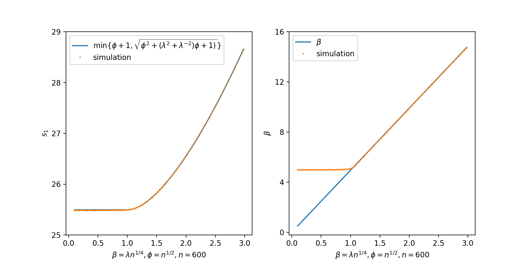
We numerically verify Theorem 3.2. We take n=600n=600, k=3k=3 and β=λ​n(k−2)/4=λ​n1/4\beta=\lambda n^{(k-2)/4}=\lambda n^{1/4} for λ∈[0,3]\lambda\in[0,3]. We sample the signals 𝒗1=𝒗2=𝒗3=𝒗{\bm{v}}_{1}={\bm{v}}_{2}={\bm{v}}_{3}={\bm{v}} as unit Gaussian vectors, and the noise tensor 𝑾\bm{W} with independent Gaussian entries. In the left panel of Figure 3, we plot the largest singular value of the unfolded matrix 𝖬𝖺𝗍i​(𝑿){\mathsf{Mat}_{i}}(\bm{X}) and our theoretical prediction (2.5). In the right panel of Figure 3 we plot β\beta and our estimator β^\hat{\beta} as in (3.7). The estimator β^\hat{\beta} provides a good approximation of β\beta provided that λ>1\lambda>1. In Figure (4) we plot |𝒗^,𝒗⟩||\hat{\bm{v}},{\bm{v}}\rangle|, where the estimator 𝒗^\hat{\bm{v}} is given as the left singular vector corresponding to the largest singular value of the unfolded matrix. Our theoretical prediction (blue curve) as in (3.9) matches well with the the simulation for λ>1\lambda>1. For λ→0\lambda\rightarrow 0, our estimator behaves as poorly as random guess, i.e. taking 𝒗^\hat{\bm{v}} as a random Gaussian vector (Green curve). For λ\lambda in a small neighborhood of 11, we don’t have a good estimation of |⟨𝒗^,𝒗⟩||\langle\hat{\bm{v}},{\bm{v}}\rangle|, but only an upper bound (3.10). In the second panel of Figure 4, we zoom in around λ=1\lambda=1, the red curve, min{n−1/6,1/n|λ−1|}\min\{n^{-1/6},1/\sqrt{n}|\lambda-1|\} corresponding to the bound (3.10), provides a good upper bound of |⟨𝒗^,𝒗⟩||\langle\hat{\bm{v}},{\bm{v}}\rangle|.

Refer to caption
Figure 3: For n=600n=600, k=3k=3, β=λ∗n(k−2)/4\beta=\lambda*n^{(k-2)/4} with λ∈[0,3]\lambda\in[0,3], averaging over 500500 trials, the left panel plots the largest singular value of the unfolded matrix and our theoretical prediction; the left panel plots the β\beta and the estimator β^\hat{\beta}.
Refer to caption
Figure 4: This plot of |⟨𝒗^,𝒗⟩||\langle\hat{{\bm{v}}},{\bm{v}}\rangle| is for n=600n=600, β=λ∗n(k−2)/4\beta=\lambda*n^{(k-2)/4} with λ∈[0,3]\lambda\in[0,3], averaging over 500500 trials.

4 Low rank Perturbations of Long Random Matrices

In this section we prove our main results as stated in Section 2. The proof of Theorem 2.2 is given in Section 4.1. We also collect the isotropic local law for long random matrices from [1]. In section 4.2, we derive a master equation which characterizes the outliers of the perturbed matrix β​𝒗​𝒖⊤+Z\beta{\bm{v}}{\bm{u}}^{\top}+Z. The master equation has been used intensively to study the low rank perturbation of random matrices, for both singular values and eigenvalues, see [10, 11, 9, 30]. The proofs of Theorems 2.3 and 2.4 are given in Sections 4.3 and 4.4 respectively.

4.1 Long Random Matrices

Let ZZ be an n×mn\times m random matrix, with entries satisfying Assumption 2.1. Let ϕ=m/n\phi=\sqrt{m/n}, with n−C⩽ϕ⩽nCn^{-C}\leqslant\phi\leqslant n^{C}. In this section we recall some results of the sample covariance matrices in this setting from [1]. It turns out in this setting the correct normalization is to study Z​Z⊤/ϕZZ^{\top}/\phi, which corresponds to the standard sample covariance matrices, with variance ϕ\phi.

We denote the following nn-dependent Marchenko-Pastur law corresponding to the ratio m/n=ϕ2⩾1m/n=\phi^{2}\geqslant 1,

ρM​Pϕ​(x)​d​x=(x−(ϕ−1ϕ)2)​((ϕ+1ϕ)2−x)2​π​x/ϕ​d​x,\displaystyle\rho^{\phi}_{MP}(x){\rm d}x=\frac{\sqrt{\left(x-\left(\sqrt{\phi}-\frac{1}{\sqrt{\phi}}\right)^{2}\right)\left(\left(\sqrt{\phi}+\frac{1}{\sqrt{\phi}}\right)^{2}-x\right)}}{2\pi x/\phi}{\rm d}x, (4.1)

and its 1/n1/n-quanties as

i−1/2n=∫νiϕ∞ρM​Pϕ​(x)​𝑑x.\displaystyle\frac{i-1/2}{n}=\int_{\nu^{\phi}_{i}}^{\infty}\rho^{\phi}_{MP}(x){\rm d}x. (4.2)

The normalization in (4.1) is different from that in (2.1), which corresponds to the sample covariance matrix Z​Z⊤ZZ^{\top}. We remark that both the Marchenko-Pastur law ϕM​Pϕ\phi_{MP}^{\phi} and its quantiles νiϕ\nu_{i}^{\phi} depend on m,nm,n through ϕ\phi. We recall the following eigenvalue rigidity result from [1, Theorem 2.10].

Theorem 4.1 (Eigenvalue Rigidity).

Under Assumption 2.1, let ϕ=m/n\phi=\sqrt{m/n} with n1/C⩽ϕ⩽nCn^{1/C}\leqslant\phi\leqslant n^{C}, the eigenvalues λ1⩾λ2⩾⋯⩾λn⩾0\lambda_{1}\geqslant\lambda_{2}\geqslant\cdots\geqslant\lambda_{n}\geqslant 0 of Z​Z⊤/ϕZZ^{\top}/\phi are close to the quantiles of the Marchenko-Pastur law (4.1): fix any ε>0\varepsilon>0 and arbitrarily small δ>0\delta>0, with high probability it holds

|λi−νiϕ|⩽nδi1/3​n2/3,\displaystyle|\lambda_{i}-\nu^{\phi}_{i}|\leqslant\frac{n^{\delta}}{i^{1/3}n^{2/3}},

uniformly for all i∈[[1,⌊(1−ε)​n⌋]]i\in[\![{1,\lfloor{(1-\varepsilon)n}\rfloor}]\!]. If in addition ϕ−1⩾c\phi-1\geqslant c for some constant c>0c>0, then with high probability, we also have

|λi−νiϕ|⩽nδ(n+1−i)1/3​n2/3,\displaystyle|\lambda_{i}-\nu^{\phi}_{i}|\leqslant\frac{n^{\delta}}{(n+1-i)^{1/3}n^{2/3}},

uniformly for all i∈[[⌊n/2⌋,n]]i\in[\![{\lfloor{n/2}\rfloor,n}]\!], provided nn is large enough.

We denote the singular values of ZZ as s1⩾s2⩾⋯⩾sn⩾0s_{1}\geqslant s_{2}\geqslant\cdots\geqslant s_{n}\geqslant 0. We can then restate Theorem 4.1 in terms of the singular values of ZZ, thanks to the following easy relation

λi=si2/ϕ,1⩽i⩽n.\displaystyle\lambda_{i}=s_{i}^{2}/\phi,\hskip 10.00002pt1\leqslant i\leqslant n. (4.3)

Theorem 2.2 is an easy consequence of Theorem 4.1 and the relation (4.3).

Proof of Theorem 2.2.

The largest singular value s1s_{1} of ZZ, and the largest eigenvalue λ1\lambda_{1} of Z​Z⊤/ϕZZ^{\top}/\phi are related by λ1=s12/ϕ\lambda_{1}=s_{1}^{2}/\phi. Therefore, Theorem 4.1 implies that |s12/ϕ−(ϕ+1/ϕ)2|⩽nδ/n2/3|s_{1}^{2}/\phi-(\sqrt{\phi}+1/\sqrt{\phi})^{2}|\leqslant n^{\delta}/n^{2/3}, with high probability, provided nn is large enough. The claim (2.3) follows from rearranging. ∎

The empirical eigenvalue distribution of Z​Z⊤/ϕZZ^{\top}/\phi is close to the Marchenko-Pastur law (4.1). Thanks to the relation (4.3), the empirical singular value distribution ∑i=1nδsi/n\sum_{i=1}^{n}\delta_{s_{i}}/n of ZZ is close to the push forward of the Marchenko-Pastur law (4.1) (after proper normalization) by the map x↦xx\mapsto\sqrt{x},

ρϕ​(x):=2​(x/ϕ)​ρM​Pϕ​(x2/ϕ)=(x2−(ϕ−1)2)​((ϕ+1)2−x2)π​x.\displaystyle\phantom{{}={}}\rho_{\phi}(x):=2(x/\phi)\rho^{\phi}_{MP}(x^{2}/\phi)=\frac{\sqrt{\left(x^{2}-\left(\phi-1\right)^{2}\right)\left(\left(\phi+1\right)^{2}-x^{2}\right)}}{\pi x}.

We remark that ρϕ\rho_{\phi} is supported on [ϕ−1,ϕ+1][\phi-1,\phi+1],

For later use, we denote the hermitization Z~\tilde{Z} of ZZ as,

Z~=[0ZZ⊤0].\displaystyle\tilde{Z}=\left[\begin{array}[]{cc}0&Z\\ Z^{\top}&0\end{array}\right].

Then Z~\tilde{Z} has m−nm-n zero eigenvalues, and its other eigenvalues are given by ±s1,±s2,⋯,±sn\pm s_{1},\pm s_{2},\cdots,\pm s_{n}. We denote the normalized Stieltjes transform of nonzero eigenvalues of Z~\tilde{Z} as

s⁡(z)=12​n​∑i=1n1z−si+1z+si,\displaystyle s(z)=\frac{1}{2n}\sum_{i=1}^{n}\frac{1}{z-s_{i}}+\frac{1}{z+s_{i}},

and the Green’s function of Z~\tilde{Z} as

G⁡(z)=(z−[0ZZ⊤0])−1=[(z−Z​Z⊤/z)−1(z−Z​Z⊤/z)−1​(Z/z)(Z⊤/z)​(z−Z​Z⊤/z)−1(z−Z⊤​Z/z)−1].\displaystyle G(z)=\left(z-\left[\begin{array}[]{cc}0&Z\\ Z^{\top}&0\end{array}\right]\right)^{-1}=\left[\begin{array}[]{cc}(z-ZZ^{\top}/z)^{-1}&(z-ZZ^{\top}/z)^{-1}(Z/z)\\ (Z^{\top}/z)(z-ZZ^{\top}/z)^{-1}&(z-Z^{\top}Z/z)^{-1}\end{array}\right].

Then thanks to Theorem 4.1, s⁡(z)s(z) is close to the Stieltjes transform of the symmetrized version of ρϕ\rho_{\phi},

mϕ​(z)=12​∫ρϕ​(x)+ρϕ​(−x)z−x​𝑑x=∫z​ρϕ​(x)z2−x2​𝑑x=∫z​ρM​Pϕ​(x)z2−x​ϕ​𝑑x.\displaystyle m_{\phi}(z)=\frac{1}{2}\int\frac{\rho_{\phi}(x)+\rho_{\phi}(-x)}{z-x}{\rm d}x=\int\frac{z\rho_{\phi}(x)}{z^{2}-x^{2}}{\rm d}x=\int\frac{z\rho_{MP}^{\phi}(x)}{z^{2}-x\phi}{\rm d}x.

More explicitly, using the formula of ρM​Pϕ\rho_{MP}^{\phi} from (4.1), mϕ​(z)m_{\phi}(z) is given by

mϕ​(z)=−(ϕ−1/ϕ)+z2/ϕ±(z2/ϕ−(ϕ+1/ϕ)2)​(z2/ϕ−(ϕ−1/ϕ)2)2​z/ϕ,\displaystyle m_{\phi}(z)=\frac{-(\phi-1/\phi)+z^{2}/\phi\pm\sqrt{(z^{2}/\phi-(\sqrt{\phi}+1/\sqrt{\phi})^{2})(z^{2}/\phi-(\sqrt{\phi}-1/\sqrt{\phi})^{2})}}{2z/\phi}, (4.10)

and it satisfies the algebraic equation

mϕ2+(ϕ2−1z−z)​mϕ+1=0.\displaystyle m_{\phi}^{2}+\left(\frac{\phi^{2}-1}{z}-z\right)m_{\phi}+1=0. (4.11)

Let z=E+i​ηz=E+\mathrm{i}\eta with κ:=min⁡{|E−(ϕ−1)|,|E−(ϕ+1)|}\kappa\mathrel{\mathop{:}}=\min\{|E-(\phi-1)|,|E-(\phi+1)|\}. We denote the spectral domains

𝑺:={z=E+iη:κ⩽𝔠−1,n−1+𝔠⩽η⩽𝔠−1},𝑺~:={z=E+iη:E∉[(ϕ−1),(ϕ+1)],n−2/3+𝔠⩽κ⩽𝔠−1,0<η⩽𝔠−1}.\displaystyle\begin{split}&\bm{S}\mathrel{\mathop{:}}=\{z=E+\mathrm{i}\eta:\kappa\leqslant{\mathfrak{c}}^{-1},n^{-1+{\mathfrak{c}}}\leqslant\eta\leqslant{\mathfrak{c}}^{-1}\},\\ &\tilde{\bm{S}}\mathrel{\mathop{:}}=\{z=E+\mathrm{i}\eta:E\not\in[(\phi-1),(\phi+1)],n^{-2/3+{\mathfrak{c}}}\leqslant\kappa\leqslant{\mathfrak{c}}^{-1},0<\eta\leqslant{\mathfrak{c}}^{-1}\}.\end{split} (4.12)

The spectral domain 𝑺\bm{S} contains the spectral information inside the bulk, and the spectral domain 𝑺~\tilde{\bm{S}} contains the spectral information close to the spectral edge. We recall the following isotropic local law from [1, Theorem 3.11, 3.12], which will be used in Sections 4.3 and 4.4.

Theorem 4.2 (Isotropic Local Law).

For unit vectors 𝐚∈ℝn{\bm{a}}\in{\mathbb{R}}^{n} and 𝐛∈ℝm{\bm{b}}\in{\mathbb{R}}^{m}, with high probability, uniformly for z∈𝐒z\in\bm{S}, we have

|⟨𝒂,(z−Z​Z⊤/z)−1​𝒂⟩−mϕ​(z)​⟨𝒂,𝒂⟩|≺|Im[mϕ​(z)]|n​η+1n​η,|⟨𝒂,(z−Z​Z⊤/z)−1​(Z/z)​𝒃⟩|≺1ϕ​(|Im[mϕ​(z)]|n​η+1n​η),|⟨𝒃,(z−Z⊤​Z/z)−1​𝒃⟩−⟨𝒃,𝒃⟩z−mϕ​(z)|≺1ϕ2​(|Im[mϕ​(z)]|n​η+1n​η).\displaystyle\begin{split}&\left|\langle{\bm{a}},(z-ZZ^{\top}/z)^{-1}{\bm{a}}\rangle-m_{\phi}(z)\langle{\bm{a}},{\bm{a}}\rangle\right|\prec\sqrt{\frac{|\mathop{\mathrm{Im}}[m_{\phi}(z)]|}{n\eta}}+\frac{1}{n\eta},\\ &\left|\langle{\bm{a}},(z-ZZ^{\top}/z)^{-1}(Z/z){\bm{b}}\rangle\right|\prec\frac{1}{\phi}\left(\sqrt{\frac{|\mathop{\mathrm{Im}}[m_{\phi}(z)]|}{n\eta}}+\frac{1}{n\eta}\right),\\ &\left|\langle{\bm{b}},(z-Z^{\top}Z/z)^{-1}{\bm{b}}\rangle-\frac{\langle{\bm{b}},{\bm{b}}\rangle}{z-m_{\phi}(z)}\right|\prec\frac{1}{\phi^{2}}\left(\sqrt{\frac{|\mathop{\mathrm{Im}}[m_{\phi}(z)]|}{n\eta}}+\frac{1}{n\eta}\right).\end{split}

Uniformly for z∈𝐒~z\in\tilde{\bm{S}} we have the improved estimates:

|⟨𝒂,(z−Z​Z⊤/z)−1​𝒂⟩−mϕ​(z)​⟨𝒂,𝒂⟩|≺|Im[mϕ​(z)]|n​η,|⟨𝒂,(z−Z​Z⊤/z)−1​(Z/z)​𝒃⟩|≺1ϕ​|Im[mϕ​(z)]|n​η,|⟨𝒃,(z−Z⊤​Z/z)−1​𝒃⟩−⟨𝒃,𝒃⟩z−mϕ​(z)|≺1ϕ2​|Im[mϕ​(z)]|n​η.\displaystyle\begin{split}&\left|\langle{\bm{a}},(z-ZZ^{\top}/z)^{-1}{\bm{a}}\rangle-m_{\phi}(z)\langle{\bm{a}},{\bm{a}}\rangle\right|\prec\sqrt{\frac{|\mathop{\mathrm{Im}}[m_{\phi}(z)]|}{n\eta}},\\ &\left|\langle{\bm{a}},(z-ZZ^{\top}/z)^{-1}(Z/z){\bm{b}}\rangle\right|\prec\frac{1}{\phi}\sqrt{\frac{|\mathop{\mathrm{Im}}[m_{\phi}(z)]|}{n\eta}},\\ &\left|\langle{\bm{b}},(z-Z^{\top}Z/z)^{-1}{\bm{b}}\rangle-\frac{\langle{\bm{b}},{\bm{b}}\rangle}{z-m_{\phi}(z)}\right|\prec\frac{1}{\phi^{2}}\sqrt{\frac{|\mathop{\mathrm{Im}}[m_{\phi}(z)]|}{n\eta}}.\end{split}

4.2 Master Equation

In this section, we derive a master equation, which characterize the outliers of the perturbed matrix β​𝒗​𝒖⊤+Z\beta{\bm{v}}{\bm{u}}^{\top}+Z. We denote the Hermitization of β​𝒗​𝒖⊤+Z\beta{\bm{v}}{\bm{u}}^{\top}+Z as

[𝒗/2𝒗​2𝒖/2−𝒖​2]​[β00−β]​[𝒗/2𝒗​2𝒖/2−𝒖​2]⊤+[0ZZ⊤0],\displaystyle\left[\begin{array}[]{cc}{\bm{v}}/\sqrt{2}&{\bm{v}}\sqrt{2}\\ {\bm{u}}/\sqrt{2}&-{\bm{u}}\sqrt{2}\end{array}\right]\left[\begin{array}[]{cc}\beta&0\\ 0&-\beta\end{array}\right]\left[\begin{array}[]{cc}{\bm{v}}/\sqrt{2}&{\bm{v}}\sqrt{2}\\ {\bm{u}}/\sqrt{2}&-{\bm{u}}\sqrt{2}\end{array}\right]^{\top}+\left[\begin{array}[]{cc}0&Z\\ Z^{\top}&0\end{array}\right],

which encodes the spectral information of β​𝒗​𝒖⊤+Z\beta{\bm{v}}{\bm{u}}^{\top}+Z. We can view (4.2) as a rank two perturbation of Z~\tilde{Z}. We have the following well-known low rank perturbation formula

Lemma 4.3.

For two (n+m)×r(n+m)\times r matrices AA and BB, it holds that

det(I−A​B⊤)=det(I−B⊤​A).\displaystyle\det(I-AB^{\top})=\det(I-B^{\top}A). (4.21)

The matrix I−A​B⊤I-AB^{\top} is invertible if and only if I−B⊤​AI-B^{\top}A is invertible, and

(I−A​B⊤)−1=I+A​(I−B⊤​A)−1​B⊤.\displaystyle(I-AB^{\top})^{-1}=I+A(I-B^{\top}A)^{-1}B^{\top}. (4.22)
Proof.

The identity (4.21) is Sylvester’s determinant theorem. And the second identity (4.22) is known as the matrix inversion lemma or Woodbury’s matrix identity. ∎

We will use Lemma 4.3 to study (4.2), which is a rank two perturbation of Z~\tilde{Z}. Its eigenvalues are given by the roots of the characteristic polynomials

det(z−[𝒗/2𝒗​2𝒖/2−𝒖​2]​[β00−β]​[𝒗/2𝒗​2𝒖/2−𝒖​2]⊤−[0ZZ⊤0])\displaystyle\phantom{{}={}}\det\left(z-\left[\begin{array}[]{cc}{\bm{v}}/\sqrt{2}&{\bm{v}}\sqrt{2}\\ {\bm{u}}/\sqrt{2}&-{\bm{u}}\sqrt{2}\end{array}\right]\left[\begin{array}[]{cc}\beta&0\\ 0&-\beta\end{array}\right]\left[\begin{array}[]{cc}{\bm{v}}/\sqrt{2}&{\bm{v}}\sqrt{2}\\ {\bm{u}}/\sqrt{2}&-{\bm{u}}\sqrt{2}\end{array}\right]^{\top}-\left[\begin{array}[]{cc}0&Z\\ Z^{\top}&0\end{array}\right]\right)
=det(z−[0ZZ⊤0])​det(I−G⁡(z)​[𝒗/2𝒗​2𝒖/2−𝒖​2]​[β00−β]​[𝒗/2𝒗​2𝒖/2−𝒖​2]⊤)\displaystyle=\det\left(z-\left[\begin{array}[]{cc}0&Z\\ Z^{\top}&0\end{array}\right]\right)\det\left(I-G(z)\left[\begin{array}[]{cc}{\bm{v}}/\sqrt{2}&{\bm{v}}\sqrt{2}\\ {\bm{u}}/\sqrt{2}&-{\bm{u}}\sqrt{2}\end{array}\right]\left[\begin{array}[]{cc}\beta&0\\ 0&-\beta\end{array}\right]\left[\begin{array}[]{cc}{\bm{v}}/\sqrt{2}&{\bm{v}}\sqrt{2}\\ {\bm{u}}/\sqrt{2}&-{\bm{u}}\sqrt{2}\end{array}\right]^{\top}\right)
=det(z−[0ZZ⊤0])​det(I−U⊤​A​(z)),\displaystyle=\det\left(z-\left[\begin{array}[]{cc}0&Z\\ Z^{\top}&0\end{array}\right]\right)\det\left(I-U^{\top}A(z)\right),

where we used Lemma 4.3 for r=2r=2, and

A⁡(z):=G⁡(z)​[𝒗/2𝒗​2𝒖/2−𝒖​2]​[β00−β],U:=[𝒗/2𝒗​2𝒖/2−𝒖​2].\displaystyle A(z):=G(z)\left[\begin{array}[]{cc}{\bm{v}}/\sqrt{2}&{\bm{v}}\sqrt{2}\\ {\bm{u}}/\sqrt{2}&-{\bm{u}}\sqrt{2}\end{array}\right]\left[\begin{array}[]{cc}\beta&0\\ 0&-\beta\end{array}\right],\hskip 10.00002ptU:=\left[\begin{array}[]{cc}{\bm{v}}/\sqrt{2}&{\bm{v}}\sqrt{2}\\ {\bm{u}}/\sqrt{2}&-{\bm{u}}\sqrt{2}\end{array}\right].

Therefore, the singular values of β​𝒖​𝒗⊤+Z\beta{\bm{u}}{\bm{v}}^{\top}+Z (which are not eigenvalues of Z~\tilde{Z}) are characterized by

det(I−U⊤​A​(z))=0.\displaystyle\det(I-U^{\top}A(z))=0. (4.29)

The equation (4.29) can be used to characterize the outliers of β​𝒗​𝒖⊤+Z\beta{\bm{v}}{\bm{u}}^{\top}+Z, and we will use it to prove Theorem 2.3 in Section 4.3.

Thanks to Lemma 4.3, for z∈ℂ+z\in{\mathbb{C}}^{+} in the upper half plane, we can write explicitly the Green’s of the Hermitization (4.2) of β​𝒗​𝒖⊤+Z\beta{\bm{v}}{\bm{u}}^{\top}+Z,

(z−[𝒗/2𝒗​2𝒖/2−𝒖​2]​[β00−β]​[𝒗/2𝒗​2𝒖/2−𝒖​2]⊤−[0ZZ⊤0])−1=(I−G⁡(z)​[𝒗/2𝒗​2𝒖/2−𝒖​2]​[β00−β]​[𝒗/2𝒗​2𝒖/2−𝒖​2]⊤)−1​G​(z)=(I+A⁡(z)​(I−U⊤​A​(z))−1​U⊤)​G​(z).\displaystyle\begin{split}&\phantom{{}={}}\left(z-\left[\begin{array}[]{cc}{\bm{v}}/\sqrt{2}&{\bm{v}}\sqrt{2}\\ {\bm{u}}/\sqrt{2}&-{\bm{u}}\sqrt{2}\end{array}\right]\left[\begin{array}[]{cc}\beta&0\\ 0&-\beta\end{array}\right]\left[\begin{array}[]{cc}{\bm{v}}/\sqrt{2}&{\bm{v}}\sqrt{2}\\ {\bm{u}}/\sqrt{2}&-{\bm{u}}\sqrt{2}\end{array}\right]^{\top}-\left[\begin{array}[]{cc}0&Z\\ Z^{\top}&0\end{array}\right]\right)^{-1}\\ &=\left(I-G(z)\left[\begin{array}[]{cc}{\bm{v}}/\sqrt{2}&{\bm{v}}\sqrt{2}\\ {\bm{u}}/\sqrt{2}&-{\bm{u}}\sqrt{2}\end{array}\right]\left[\begin{array}[]{cc}\beta&0\\ 0&-\beta\end{array}\right]\left[\begin{array}[]{cc}{\bm{v}}/\sqrt{2}&{\bm{v}}\sqrt{2}\\ {\bm{u}}/\sqrt{2}&-{\bm{u}}\sqrt{2}\end{array}\right]^{\top}\right)^{-1}G(z)\\ &=\left(I+A(z)(I-U^{\top}A(z))^{-1}U^{\top}\right)G(z).\end{split} (4.30)

The Green’s function (4.30) contains the information of eigenvectors, and can be used to study the singular vectors of the outliers of β​𝒗​𝒖⊤+Z\beta{\bm{v}}{\bm{u}}^{\top}+Z. And we will use it to prove Theorem 2.4 in Section 4.4.

4.3 Proof of Theorem 2.3

Let ϕ=m/n\phi=\sqrt{m/n}. We denote the singular values of β​𝒗​𝒖⊤+Z\beta{\bm{v}}{\bm{u}}^{\top}+Z as s^1⩾s^2⩾⋯⩾s^n⩾0\hat{s}_{1}\geqslant\hat{s}_{2}\geqslant\cdots\geqslant\hat{s}_{n}\geqslant 0, with corresponding normalized left and right singular vectors as 𝒗^1,𝒗^2,⋯,𝒗^n∈ℝn\hat{\bm{v}}_{1},\hat{\bm{v}}_{2},\cdots,\hat{\bm{v}}_{n}\in{\mathbb{R}}^{n}, and 𝒖^1,𝒖^2,⋯,𝒖^n∈ℝm\hat{\bm{u}}_{1},\hat{\bm{u}}_{2},\cdots,\hat{\bm{u}}_{n}\in{\mathbb{R}}^{m}. Then the nonzero eigenvalues of its Hermitization

[𝒗/2𝒗​2𝒖/2−𝒖​2]​[β00−β]​[𝒗/2𝒗​2𝒖/2−𝒖​2]⊤+[0ZZ⊤0],\displaystyle\left[\begin{array}[]{cc}{\bm{v}}/\sqrt{2}&{\bm{v}}\sqrt{2}\\ {\bm{u}}/\sqrt{2}&-{\bm{u}}\sqrt{2}\end{array}\right]\left[\begin{array}[]{cc}\beta&0\\ 0&-\beta\end{array}\right]\left[\begin{array}[]{cc}{\bm{v}}/\sqrt{2}&{\bm{v}}\sqrt{2}\\ {\bm{u}}/\sqrt{2}&-{\bm{u}}\sqrt{2}\end{array}\right]^{\top}+\left[\begin{array}[]{cc}0&Z\\ Z^{\top}&0\end{array}\right],

are given by s^1,−s^1,s^2,−s^2,⋯,s^n,−s^n\hat{s}_{1},-\hat{s}_{1},\hat{s}_{2},-\hat{s}_{2},\cdots,\hat{s}_{n},-\hat{s}_{n}. The corresponding normalized eigenvectors are given by [𝒗^1,𝒖^1]/2,[𝒗^1,−𝒖^1]/2,[𝒗^2,𝒖^2]/2,[𝒗^2,−𝒖^2]/2,⋯,[𝒗^n,𝒖^n]/2,[𝒗^n,−𝒖^n]/2[\hat{\bm{v}}_{1},\hat{\bm{u}}_{1}]/\sqrt{2},[\hat{\bm{v}}_{1},-\hat{\bm{u}}_{1}]/\sqrt{2},[\hat{\bm{v}}_{2},\hat{\bm{u}}_{2}]/\sqrt{2},[\hat{\bm{v}}_{2},-\hat{\bm{u}}_{2}]/\sqrt{2},\cdots,[\hat{\bm{v}}_{n},\hat{\bm{u}}_{n}]/\sqrt{2},[\hat{\bm{v}}_{n},-\hat{\bm{u}}_{n}]/\sqrt{2}.

We recall from Theorem 4.1 that with high probability the singular values of ZZ are bounded by (ϕ+1)+n−2/3+𝔠/2(\phi+1)+n^{-2/3+{\mathfrak{c}}/2}, i.e. s1⩽(ϕ+1)+n−2/3+𝔠/2s_{1}\leqslant(\phi+1)+n^{-2/3+{\mathfrak{c}}/2}. In the remaining of this section, we restrict ourselves to the event that s1⩽(ϕ+1)+n−2/3+𝔠/2s_{1}\leqslant(\phi+1)+n^{-2/3+{\mathfrak{c}}/2}, which holds with high probability. We can view (4.3) as a rank two perturbation of Z~\tilde{Z},

β⁡[𝒗/2𝒖/2]​[𝒗/2𝒖/2]⊤−β⁡[𝒗/2−𝒖/2]​[𝒗/2−𝒖/2]⊤+[0ZZ⊤0],\displaystyle\beta\left[\begin{array}[]{c}{\bm{v}}/\sqrt{2}\\ {\bm{u}}/\sqrt{2}\end{array}\right]\left[\begin{array}[]{c}{\bm{v}}/\sqrt{2}\\ {\bm{u}}/\sqrt{2}\end{array}\right]^{\top}-\beta\left[\begin{array}[]{c}{\bm{v}}/\sqrt{2}\\ -{\bm{u}}/\sqrt{2}\end{array}\right]\left[\begin{array}[]{c}{\bm{v}}/\sqrt{2}\\ -{\bm{u}}/\sqrt{2}\end{array}\right]^{\top}+\left[\begin{array}[]{cc}0&Z\\ Z^{\top}&0\end{array}\right],

By the variational formula of eigenvalues, s^2\hat{s}_{2} is upper bounded by the second largest eigenvalue of

β⁡[𝒗/2𝒖/2]​[𝒗/2𝒖/2]⊤+[0ZZ⊤0].\displaystyle\beta\left[\begin{array}[]{c}{\bm{v}}/\sqrt{2}\\ {\bm{u}}/\sqrt{2}\end{array}\right]\left[\begin{array}[]{c}{\bm{v}}/\sqrt{2}\\ {\bm{u}}/\sqrt{2}\end{array}\right]^{\top}+\left[\begin{array}[]{cc}0&Z\\ Z^{\top}&0\end{array}\right].

Again the second largest eigenvalue of (4.3) is upper bounded by s1s_{1}. Thus we have s^2⩽s1⩽(ϕ+1)+n−2/3+𝔠/2\hat{s}_{2}\leqslant s_{1}\leqslant(\phi+1)+n^{-2/3+{\mathfrak{c}}/2}. Therefore, (4.3) can have at most one outlier eigenvalue.

We recall from (4.29), the matrix β​𝒗​𝒖⊤+Z\beta{\bm{v}}{\bm{u}}^{\top}+Z has an outlier singular value bigger than (ϕ+1)+n−2/3+𝔠(\phi+1)+n^{-2/3+{\mathfrak{c}}}, if and only if

det(I−U⊤​A​(x))=0\displaystyle\det(I-U^{\top}A(x))=0 (4.55)

has an zero with x⩾(ϕ+1)+n−2/3+𝔠x\geqslant(\phi+1)+n^{-2/3+{\mathfrak{c}}}, where

A⁡(z)=G⁡(z)​[𝒗/2𝒗​2𝒖/2−𝒖​2]​[β00−β],U=[𝒗/2𝒗​2𝒖/2−𝒖​2].\displaystyle A(z)=G(z)\left[\begin{array}[]{cc}{\bm{v}}/\sqrt{2}&{\bm{v}}\sqrt{2}\\ {\bm{u}}/\sqrt{2}&-{\bm{u}}\sqrt{2}\end{array}\right]\left[\begin{array}[]{cc}\beta&0\\ 0&-\beta\end{array}\right],\hskip 10.00002ptU=\left[\begin{array}[]{cc}{\bm{v}}/\sqrt{2}&{\bm{v}}\sqrt{2}\\ {\bm{u}}/\sqrt{2}&-{\bm{u}}\sqrt{2}\end{array}\right].

We can rewrite the equation (4.55) as

det([1/β00−1/β]−[𝒗/2𝒗​2𝒖/2−𝒖​2]⊤​G​(x)​[𝒗/2𝒗​2𝒖/2−𝒖​2])=0.\displaystyle\det\left(\left[\begin{array}[]{cc}1/\beta&0\\ 0&-1/\beta\end{array}\right]-\left[\begin{array}[]{cc}{\bm{v}}/\sqrt{2}&{\bm{v}}\sqrt{2}\\ {\bm{u}}/\sqrt{2}&-{\bm{u}}\sqrt{2}\end{array}\right]^{\top}G(x)\left[\begin{array}[]{cc}{\bm{v}}/\sqrt{2}&{\bm{v}}\sqrt{2}\\ {\bm{u}}/\sqrt{2}&-{\bm{u}}\sqrt{2}\end{array}\right]\right)=0.

We recall the Green’s function G⁡(x)G(x) from (4.1)

G⁡(x)=(x−[0ZZ⊤0])−1=[(x−Z​Z⊤/x)−1(x−Z​Z⊤/x)−1​(Z/x)(Z⊤/x)​(x−Z​Z⊤/x)−1(x−Z⊤​Z/x)−1],\displaystyle G(x)=\left(x-\left[\begin{array}[]{cc}0&Z\\ Z^{\top}&0\end{array}\right]\right)^{-1}=\left[\begin{array}[]{cc}(x-ZZ^{\top}/x)^{-1}&(x-ZZ^{\top}/x)^{-1}(Z/x)\\ (Z^{\top}/x)(x-ZZ^{\top}/x)^{-1}&(x-Z^{\top}Z/x)^{-1}\end{array}\right],

and denote the quantities

𝒜⁡(x)=⟨𝒗,(x−Z​Z⊤/x)−1​𝒗⟩,ℬ⁡(x)=⟨𝒗,(x−Z​Z⊤/x)−1​(Z/x)​𝒖⟩,𝒞⁡(x)=⟨𝒖,(x−Z⊤​Z/x)−1​𝒖⟩\displaystyle\begin{split}&{\mathcal{A}}(x)=\langle{\bm{v}},(x-ZZ^{\top}/x)^{-1}{\bm{v}}\rangle,\\ &{\mathcal{B}}(x)=\langle{\bm{v}},(x-ZZ^{\top}/x)^{-1}(Z/x){\bm{u}}\rangle,\\ &{\mathcal{C}}(x)=\langle{\bm{u}},(x-Z^{\top}Z/x)^{-1}{\bm{u}}\rangle\end{split} (4.62)

With these notations, we can rewrite (4.3) as

det([1/β00−1/β]−12​[𝒜⁡(x)+2​ℬ​(x)+𝒞⁡(x)𝒜⁡(x)−𝒞⁡(x)𝒜⁡(x)−𝒞⁡(x)𝒜⁡(x)−2​ℬ​(x)+𝒞⁡(x)])=0.\displaystyle\det\left(\left[\begin{array}[]{cc}1/\beta&0\\ 0&-1/\beta\end{array}\right]-\frac{1}{2}\left[\begin{array}[]{cc}{\mathcal{A}}(x)+2{\mathcal{B}}(x)+{\mathcal{C}}(x)&{\mathcal{A}}(x)-{\mathcal{C}}(x)\\ {\mathcal{A}}(x)-{\mathcal{C}}(x)&{\mathcal{A}}(x)-2{\mathcal{B}}(x)+{\mathcal{C}}(x)\end{array}\right]\right)=0.

It simplifies to

(1β−ℬ⁡(x))2=𝒜⁡(x)​𝒞​(x).\displaystyle\left(\frac{1}{\beta}-{\mathcal{B}}(x)\right)^{2}={\mathcal{A}}(x){\mathcal{C}}(x). (4.67)

Let x−(ϕ+1)=κ⩾n−2/3+𝔠x-(\phi+1)=\kappa\geqslant n^{-2/3+{\mathfrak{c}}}, then x∈𝑺~x\in\tilde{\bm{S}} as defined in (4.12). Thanks to the Square root behavior (4.10) of mϕ​(z)m_{\phi}(z) around the spectral edge z=ϕ+1z=\phi+1, we have

|Im[mϕ​(z)]|≍ηκ+η,z=ϕ+1+κ+i​η,κ⩾0.\displaystyle|\mathop{\mathrm{Im}}[m_{\phi}(z)]|\asymp\frac{\eta}{\sqrt{\kappa+\eta}},\hskip 10.00002ptz=\phi+1+\kappa+\mathrm{i}\eta,\hskip 10.00002pt\kappa\geqslant 0.

In particular we have

|Im[mϕ​(z)]|n​η≍1n1/2​κ1/4,z=ϕ+1+κ+i​η,κ⩾0.\displaystyle\sqrt{\frac{|\mathop{\mathrm{Im}}[m_{\phi}(z)]|}{n\eta}}\asymp\frac{1}{n^{1/2}\kappa^{1/4}},\hskip 10.00002ptz=\phi+1+\kappa+\mathrm{i}\eta,\hskip 10.00002pt\kappa\geqslant 0. (4.68)

Thanks to Theorem 4.2 with 𝒂=𝒗{\bm{a}}={\bm{v}} and 𝒃=𝒖{\bm{b}}={\bm{u}}, by plugging (4.68), we have

𝒜⁡(x)=mϕ​(x)+O≺⁡(1n1/2​κ1/4),ℬ⁡(x)=O≺⁡(1ϕ​n1/2​κ1/4),𝒞⁡(x)=1x−mϕ​(x)+O≺⁡(1ϕ2​n1/2​κ1/4),\displaystyle\begin{split}&{\mathcal{A}}(x)=m_{\phi}(x)+\OO_{\prec}\left(\frac{1}{n^{1/2}\kappa^{1/4}}\right),\\ &{\mathcal{B}}(x)=\OO_{\prec}\left(\frac{1}{\phi n^{1/2}\kappa^{1/4}}\right),\\ &{\mathcal{C}}(x)=\frac{1}{x-m_{\phi}(x)}+\OO_{\prec}\left(\frac{1}{\phi^{2}n^{1/2}\kappa^{1/4}}\right),\end{split} (4.69)

where the error terms are continuous in xx. Then by plugging (4.69) we can rewrite (4.67) as

1β2=mϕ​(x)x−mϕ​(x)+O≺⁡(1ϕ​n1/2​κ1/4).\displaystyle\frac{1}{\beta^{2}}=\frac{m_{\phi}(x)}{x-m_{\phi}(x)}+\OO_{\prec}\left(\frac{1}{\phi n^{1/2}\kappa^{1/4}}\right). (4.70)

We recall the algebraic equation of mϕm_{\phi} from (4.11)

mϕ2+(ϕ2−1x−x)​mϕ+1=0,\displaystyle m_{\phi}^{2}+\left(\frac{\phi^{2}-1}{x}-x\right)m_{\phi}+1=0, (4.71)

By further rearranging (4.70) we get

mϕ​(x)x−mϕ​(x)=1β2+O≺⁡(1ϕ​n1/2​κ1/4).\displaystyle\frac{m_{\phi}(x)}{x-m_{\phi}(x)}=\frac{1}{\beta^{2}}+\OO_{\prec}\left(\frac{1}{\phi n^{1/2}\kappa^{1/4}}\right). (4.72)

Since mϕ​(x)m_{\phi}(x) is monotone decreasing for x⩾ϕ+1x\geqslant\phi+1, the lefthand side is monotone decreasing for x⩾ϕ+1x\geqslant\phi+1. Using the formula (4.10) for mϕ​(x)m_{\phi}(x), for x=ϕ+1x=\phi+1, mϕ​(x)=1m_{\phi}(x)=1. For x→∞x\rightarrow\infty, we have mϕ​(x)→0m_{\phi}(x)\rightarrow 0. And for x=ϕ+1+κx=\phi+1+\kappa, with κ=o⁡(1)\kappa=\oo(1), we have

mϕ​(x)=1−C​κ+O⁡(κ),\displaystyle m_{\phi}(x)=1-C\sqrt{\kappa}+\OO(\kappa),

for some constant C>0C>0. In this regime, the lefthand side of (4.72) behaves

mϕ​(x)x−mϕ​(x)=1−C​κ+O⁡(κ)ϕ+C​κ+O⁡(κ)=1ϕ​(1−(C+C/ϕ)​κ+O⁡(κ))\displaystyle\frac{m_{\phi}(x)}{x-m_{\phi}(x)}=\frac{1-C\sqrt{\kappa}+\OO(\kappa)}{\phi+C\sqrt{\kappa}+\OO(\kappa)}=\frac{1}{\phi}\left(1-(C+C/\phi)\sqrt{\kappa}+\OO(\kappa)\right) (4.73)

We take

β=λ​ϕ.\displaystyle\beta=\lambda\sqrt{\phi}.

In the following we first prove (2.6).

Proof of (2.6).

If λ⩽1+n−1/3+𝔠\lambda\leqslant 1+n^{-1/3+{\mathfrak{c}}}, in the following we show that (4.70) does not have solution with x⩾ϕ+1+n−2/3+3𝔠x\geqslant\phi+1+n^{-2/3+3{\mathfrak{c}}}. For x⩾ϕ+1+n−2/3+3𝔠x\geqslant\phi+1+n^{-2/3+3{\mathfrak{c}}}, using (4.73) and the monotonicity of mϕ​(x)m_{\phi}(x), we have

mϕ​(x)x−mϕ​(x)⩽mϕ(ϕ+1+n−2/3+3𝔠)ϕ+1+n−2/3+3𝔠−mϕ(ϕ+1+n−2/3+3𝔠)=1ϕ(1−(C+C/ϕ)n−1/3+3𝔠/2+O(n−2/3+3𝔠)).\displaystyle\begin{split}\frac{m_{\phi}(x)}{x-m_{\phi}(x)}&\leqslant\frac{m_{\phi}(\phi+1+n^{-2/3+3{\mathfrak{c}}})}{\phi+1+n^{-2/3+3{\mathfrak{c}}}-m_{\phi}(\phi+1+n^{-2/3+3{\mathfrak{c}}})}\\ &=\frac{1}{\phi}(1-(C+C/\phi)n^{-1/3+3{\mathfrak{c}}/2}+\OO(n^{-2/3+3{\mathfrak{c}}})).\end{split} (4.74)

For x⩾ϕ+1+n−2/3+3𝔠x\geqslant\phi+1+n^{-2/3+3{\mathfrak{c}}}, the righthand side of (4.72) is lower bounded by

1β2+O≺⁡(1ϕ​n1/2​κ1/4)=1λ2​ϕ+O≺⁡(1ϕ​n1/2​κ1/4)⩾1ϕ(1−2n−1/3+𝔠+O(n−2/3+2𝔠))+O≺(1ϕ​n1/3+3​𝔠/4)>mϕ​(x)x−mϕ​(x).\displaystyle\begin{split}&\phantom{{}={}}\frac{1}{\beta^{2}}+\OO_{\prec}\left(\frac{1}{\phi n^{1/2}\kappa^{1/4}}\right)=\frac{1}{\lambda^{2}\phi}+\OO_{\prec}\left(\frac{1}{\phi n^{1/2}\kappa^{1/4}}\right)\\ &\geqslant\frac{1}{\phi}(1-2n^{-1/3+{\mathfrak{c}}}+\OO(n^{-2/3+2{\mathfrak{c}}}))+\OO_{\prec}\left(\frac{1}{\phi n^{1/3+3{\mathfrak{c}}/4}}\right)>\frac{m_{\phi}(x)}{x-m_{\phi}(x)}.\end{split} (4.75)

Therefore, (4.72) does not have solution for x⩾ϕ+1+n−2/3+3𝔠x\geqslant\phi+1+n^{-2/3+3{\mathfrak{c}}}. We conclude that s^1⩽ϕ+1+n−2/3+3𝔠\hat{s}_{1}\leqslant\phi+1+n^{-2/3+3{\mathfrak{c}}}. This finishes the proof (2.6). ∎

In the following, we study the case that λ⩾1+n−1/3+𝔠\lambda\geqslant 1+n^{-1/3+{\mathfrak{c}}}.

Proof of (2.5).

Similarly to (4.74) and (4.75) we have for x=ϕ+1+n−2/3+𝔠x=\phi+1+n^{-2/3+{\mathfrak{c}}}

1β2+O≺⁡(1ϕ​n1/2​κ1/4)⩽mϕ​(x)x−mϕ​(x).\displaystyle\frac{1}{\beta^{2}}+\OO_{\prec}\left(\frac{1}{\phi n^{1/2}\kappa^{1/4}}\right)\leqslant\frac{m_{\phi}(x)}{x-m_{\phi}(x)}.

And for x→∞x\rightarrow\infty,

limx→∞1β2+O≺⁡(1ϕ​n1/2​κ1/4)=1β2⩾limx→∞mϕ​(x)x−mϕ​(x)=0.\displaystyle\lim_{x\rightarrow\infty}\frac{1}{\beta^{2}}+\OO_{\prec}\left(\frac{1}{\phi n^{1/2}\kappa^{1/4}}\right)=\frac{1}{\beta^{2}}\geqslant\lim_{x\rightarrow\infty}\frac{m_{\phi}(x)}{x-m_{\phi}(x)}=0.

Therefore (4.72) a has a solution in the interval [ϕ+1+n−2/3+𝔠,∞)[\phi+1+n^{-2/3+{\mathfrak{c}}},\infty), which is s^1\hat{s}_{1}. In particularly we have s^1⩾ϕ+1+n−2/3+𝔠\hat{s}_{1}\geqslant\phi+1+n^{-2/3+{\mathfrak{c}}}, and β​𝒗​𝒖⊤+Z\beta{\bm{v}}{\bm{u}}^{\top}+Z has an outlier. In the following, we compute the value of s^1\hat{s}_{1}.

We rewrite the equation (4.72) as

mϕ​(x)x−mϕ​(x)=τϕ,τ=1λ2+O≺⁡(1n1/2​κ1/4).\displaystyle\frac{m_{\phi}(x)}{x-m_{\phi}(x)}=\frac{\tau}{\phi},\hskip 10.00002pt\tau=\frac{1}{\lambda^{2}}+\OO_{\prec}\left(\frac{1}{n^{1/2}\kappa^{1/4}}\right). (4.76)

We can solve for xx and mϕ​(x)m_{\phi}(x) using (4.71) and (4.76)

x=ϕ2+(τ+1/τ)​ϕ+1=ϕ2+(λ2+1/λ2)​ϕ+1+O≺⁡((λ−1)ϕ​1n1/2​κ1/4+1ϕ​1n​κ1/2),mϕ=x1+ϕ/τ=(1+O≺⁡(1n1/2​κ1/4))​ϕ+λ2λ2​(1+λ2​ϕ).\displaystyle\begin{split}&x=\sqrt{\phi^{2}+(\tau+1/\tau)\phi+1}=\sqrt{\phi^{2}+(\lambda^{2}+1/\lambda^{2})\phi+1}+\OO_{\prec}\left(\frac{(\lambda-1)}{\phi}\frac{1}{n^{1/2}\kappa^{1/4}}+\frac{1}{\phi}\frac{1}{n\kappa^{1/2}}\right),\\ &m_{\phi}=\frac{x}{1+\phi/\tau}=\left(1+\OO_{\prec}\left(\frac{1}{n^{1/2}\kappa^{1/4}}\right)\right)\sqrt{\frac{\phi+\lambda^{2}}{\lambda^{2}(1+\lambda^{2}\phi)}}.\end{split} (4.77)

We recall that

x=ϕ+1+κ,κ⩾n−2/3+𝔠\displaystyle x=\phi+1+\kappa,\hskip 10.00002pt\kappa\geqslant n^{-2/3+{\mathfrak{c}}}

By a Taylor expansion of the first estimate in (4.77), for λ=1+o⁡(1)\lambda=1+\oo(1), there exists some constant C>0C>0,

x⩾ϕ+1+C​(λ−1)2+O≺⁡((λ−1)ϕ​1n1/2​κ1/4+1ϕ​1n​κ1/2)\displaystyle x\geqslant\phi+1+C(\lambda-1)^{2}+\OO_{\prec}\left(\frac{(\lambda-1)}{\phi}\frac{1}{n^{1/2}\kappa^{1/4}}+\frac{1}{\phi}\frac{1}{n\kappa^{1/2}}\right)

By our assumption that λ⩾1+n−1/3+𝔠\lambda\geqslant 1+n^{-1/3+{\mathfrak{c}}}. Then we have κ=x−ϕ−1≍(λ−1)2≳n−2/3+2𝔠\kappa=x-\phi-1\asymp(\lambda-1)^{2}\gtrsim n^{-2/3+2{\mathfrak{c}}}. We can use this estimate of κ\kappa to simplify the error terms in (4.77). In summary we have for β=λ​ϕ\beta=\lambda\sqrt{\phi} and λ⩾1+n−1/3+𝔠\lambda\geqslant 1+n^{-1/3+{\mathfrak{c}}}, β​𝒗​𝒖⊤+Z\beta{\bm{v}}{\bm{u}}^{\top}+Z has an outlier singular value at

x=ϕ2+(λ2+1/λ2)​ϕ+1+O≺⁡((λ−1)1/2n1/2​ϕ)\displaystyle x=\sqrt{\phi^{2}+(\lambda^{2}+1/\lambda^{2})\phi+1}+\OO_{\prec}\left(\frac{(\lambda-1)^{1/2}}{n^{1/2}\phi}\right)

This finishes the proof of (2.5). ∎

4.4 Proof of Theorem 2.4

Let ϕ=m/n\phi=\sqrt{m/n}. We first study the case that λ⩾1+n−1/3+𝔠\lambda\geqslant 1+n^{-1/3+{\mathfrak{c}}}.

Proof of (2.7) and (2.8).

If λ⩾1+n−1/3+𝔠\lambda\geqslant 1+n^{-1/3+{\mathfrak{c}}}, Theorem (2.3) implies that β​𝒗​𝒖⊤+Z\beta{\bm{v}}{\bm{u}}^{\top}+Z has an outlier singular value x=s^1=ϕ+1+κx=\hat{s}_{1}=\phi+1+\kappa with κ≍(λ−1)2\kappa\asymp(\lambda-1)^{2}. Therefore, xx is an eigenvalue of the Hermitized matrix:

x​𝒘=([𝒗/2𝒗​2𝒖/2−𝒖​2]​[β00−β]​[𝒗/2𝒗​2𝒖/2−𝒖​2]⊤+[0ZZ⊤0])​𝒘,\displaystyle x{\bm{w}}=\left(\left[\begin{array}[]{cc}{\bm{v}}/\sqrt{2}&{\bm{v}}\sqrt{2}\\ {\bm{u}}/\sqrt{2}&-{\bm{u}}\sqrt{2}\end{array}\right]\left[\begin{array}[]{cc}\beta&0\\ 0&-\beta\end{array}\right]\left[\begin{array}[]{cc}{\bm{v}}/\sqrt{2}&{\bm{v}}\sqrt{2}\\ {\bm{u}}/\sqrt{2}&-{\bm{u}}\sqrt{2}\end{array}\right]^{\top}+\left[\begin{array}[]{cc}0&Z\\ Z^{\top}&0\end{array}\right]\right){\bm{w}},

for some unit vector 𝒘=[𝒗^1,𝒖^1]⊤/2{\bm{w}}=[\hat{\bm{v}}_{1},\hat{\bm{u}}_{1}]^{\top}/\sqrt{2}, where 𝒗^1,𝒖^1\hat{\bm{v}}_{1},\hat{\bm{u}}_{1} are the left and right singular vector of β​𝒗​𝒖⊤+Z\beta{\bm{v}}{\bm{u}}^{\top}+Z corresponding to the singular value s^1\hat{s}_{1}. By rearranging (4.4), we get

𝒘=(x−[0ZZ⊤0])−1​[𝒗/2𝒗​2𝒖/2−𝒖​2]​[β00−β]​[𝒗/2𝒗​2𝒖/2−𝒖​2]⊤​𝒘.\displaystyle{\bm{w}}=\left(x-\left[\begin{array}[]{cc}0&Z\\ Z^{\top}&0\end{array}\right]\right)^{-1}\left[\begin{array}[]{cc}{\bm{v}}/\sqrt{2}&{\bm{v}}\sqrt{2}\\ {\bm{u}}/\sqrt{2}&-{\bm{u}}\sqrt{2}\end{array}\right]\left[\begin{array}[]{cc}\beta&0\\ 0&-\beta\end{array}\right]\left[\begin{array}[]{cc}{\bm{v}}/\sqrt{2}&{\bm{v}}\sqrt{2}\\ {\bm{u}}/\sqrt{2}&-{\bm{u}}\sqrt{2}\end{array}\right]^{\top}{\bm{w}}.

We denote the length two vector which is the projection of 𝒘{\bm{w}} on 𝒗{\bm{v}} and 𝒖{\bm{u}} direction

𝒘~=[𝒗/2𝒗​2𝒖/2−𝒖​2]⊤​𝒘=12​[𝒗𝒗𝒖−𝒖]⊤​[𝒗^1𝒖^1],\displaystyle\tilde{\bm{w}}=\left[\begin{array}[]{cc}{\bm{v}}/\sqrt{2}&{\bm{v}}\sqrt{2}\\ {\bm{u}}/\sqrt{2}&-{\bm{u}}\sqrt{2}\end{array}\right]^{\top}{\bm{w}}=\frac{1}{2}\left[\begin{array}[]{cc}{\bm{v}}&{\bm{v}}\\ {\bm{u}}&-{\bm{u}}\end{array}\right]^{\top}\left[\begin{array}[]{c}\hat{\bm{v}}_{1}\\ \hat{\bm{u}}_{1}\end{array}\right],

then it satisfies

𝒘~=[𝒗/2𝒗​2𝒖/2−𝒖​2]⊤​(x−[0ZZ⊤0])−1​[𝒗/2𝒗​2𝒖/2−𝒖​2]​[β00−β]​𝒘~.\displaystyle\tilde{\bm{w}}=\left[\begin{array}[]{cc}{\bm{v}}/\sqrt{2}&{\bm{v}}\sqrt{2}\\ {\bm{u}}/\sqrt{2}&-{\bm{u}}\sqrt{2}\end{array}\right]^{\top}\left(x-\left[\begin{array}[]{cc}0&Z\\ Z^{\top}&0\end{array}\right]\right)^{-1}\left[\begin{array}[]{cc}{\bm{v}}/\sqrt{2}&{\bm{v}}\sqrt{2}\\ {\bm{u}}/\sqrt{2}&-{\bm{u}}\sqrt{2}\end{array}\right]\left[\begin{array}[]{cc}\beta&0\\ 0&-\beta\end{array}\right]\tilde{\bm{w}}.

We denote 𝒘~=[𝒘~1,𝒘~2]⊤\tilde{\bm{w}}=[\tilde{\bm{w}}_{1},\tilde{\bm{w}}_{2}]^{\top} with 𝒘~1∈ℝn\tilde{\bm{w}}_{1}\in{\mathbb{R}}^{n} and 𝒘~2∈ℝm\tilde{\bm{w}}_{2}\in{\mathbb{R}}^{m}. The inner products ⟨𝒗^1,𝒗⟩\langle\hat{{\bm{v}}}_{1},{\bm{v}}\rangle and ⟨𝒖^1,𝒖⟩\langle\hat{{\bm{u}}}_{1},{\bm{u}}\rangle are given by

⟨𝒗^1,𝒗⟩=𝒘~1+𝒘~2,⟨𝒖^1,𝒖⟩=𝒘~1−𝒘~2.\displaystyle\langle\hat{{\bm{v}}}_{1},{\bm{v}}\rangle=\tilde{\bm{w}}_{1}+\tilde{\bm{w}}_{2},\hskip 10.00002pt\langle\hat{{\bm{u}}}_{1},{\bm{u}}\rangle=\tilde{\bm{w}}_{1}-\tilde{\bm{w}}_{2}. (4.102)

By taking norm on both sides of (4.4), we get another equation for w~\tilde{w},

1=𝒘~⊤​[β00−β]​[𝒗/2𝒗​2𝒖/2−𝒖​2]⊤​(x−[0ZZ⊤0])−2​[𝒗/2𝒗​2𝒖/2−𝒖​2]​[β00−β]​𝒘~.\displaystyle 1=\tilde{\bm{w}}^{\top}\left[\begin{array}[]{cc}\beta&0\\ 0&-\beta\end{array}\right]\left[\begin{array}[]{cc}{\bm{v}}/\sqrt{2}&{\bm{v}}\sqrt{2}\\ {\bm{u}}/\sqrt{2}&-{\bm{u}}\sqrt{2}\end{array}\right]^{\top}\left(x-\left[\begin{array}[]{cc}0&Z\\ Z^{\top}&0\end{array}\right]\right)^{-2}\left[\begin{array}[]{cc}{\bm{v}}/\sqrt{2}&{\bm{v}}\sqrt{2}\\ {\bm{u}}/\sqrt{2}&-{\bm{u}}\sqrt{2}\end{array}\right]\left[\begin{array}[]{cc}\beta&0\\ 0&-\beta\end{array}\right]\tilde{\bm{w}}.

Using the notations from (4.62), we can rewrite (4.4) as

𝒘~=12​[𝒜⁡(x)+2​ℬ​(x)+𝒞⁡(x)𝒜⁡(x)−𝒞⁡(x)𝒜⁡(x)−𝒞⁡(x)𝒜⁡(x)−2​ℬ​(x)+𝒞⁡(x)]​[β00−β]​𝒘~,\displaystyle\tilde{\bm{w}}=\frac{1}{2}\left[\begin{array}[]{cc}{\mathcal{A}}(x)+2{\mathcal{B}}(x)+{\mathcal{C}}(x)&{\mathcal{A}}(x)-{\mathcal{C}}(x)\\ {\mathcal{A}}(x)-{\mathcal{C}}(x)&{\mathcal{A}}(x)-2{\mathcal{B}}(x)+{\mathcal{C}}(x)\end{array}\right]\left[\begin{array}[]{cc}\beta&0\\ 0&-\beta\end{array}\right]\tilde{\bm{w}},

where we recall from (4.67)

(1β−ℬ⁡(x))2=𝒜⁡(x)​𝒞​(x).\displaystyle\left(\frac{1}{\beta}-{\mathcal{B}}(x)\right)^{2}={\mathcal{A}}(x){\mathcal{C}}(x). (4.117)

Thanks to Theorem 4.2, for x=ϕ+1+κx=\phi+1+\kappa with κ⩾n−2/3+𝔠\kappa\geqslant n^{-2/3+{\mathfrak{c}}}, we have

𝒜⁡(x)=mϕ​(x)+O≺⁡(1n1/2​κ1/4),OPENℬ⁡(x)=O≺⁡(1ϕ​n1/2​κ1/4)),𝒞⁡(x)=1x−mϕ​(x)+O≺⁡(1ϕ2​n1/2​κ1/4),\displaystyle\begin{split}&{\mathcal{A}}(x)=m_{\phi}(x)+\OO_{\prec}\left(\frac{1}{n^{1/2}\kappa^{1/4}}\right),\\ &{\mathcal{B}}(x)=\OO_{\prec}\left(\frac{1}{\phi n^{1/2}\kappa^{1/4}}\right)),\\ &{\mathcal{C}}(x)=\frac{1}{x-m_{\phi}(x)}+\OO_{\prec}\left(\frac{1}{\phi^{2}n^{1/2}\kappa^{1/4}}\right),\end{split} (4.118)

where we used (4.68).

On the event that the singular values of ZZ are bounded by (ϕ+1)+n−2/3+𝔠/2(\phi+1)+n^{-2/3+{\mathfrak{c}}/2}, i.e. s1⩽(ϕ+1)+n−2/3+𝔠/2s_{1}\leqslant(\phi+1)+n^{-2/3+{\mathfrak{c}}/2}, we have that 𝒜⁡(z),ℬ⁡(z),𝒞⁡(z){\mathcal{A}}(z),{\mathcal{B}}(z),{\mathcal{C}}(z) are analytic for Re[z]⩾(ϕ+1)+n−2/3+𝔠/2\mathop{\mathrm{Re}}[z]\geqslant(\phi+1)+n^{-2/3+{\mathfrak{c}}/2}. We take a contour ω={z:|z−x|=κ/2}\omega=\{z:|z-x|=\kappa/2\}. Inside the contour Re[z]⩾ϕ+1+n−2/3+𝔠/2\mathop{\mathrm{Re}}[z]\geqslant\phi+1+n^{-2/3+{\mathfrak{c}}}/2, 𝒜⁡(z){\mathcal{A}}(z) is analytic. Then we can rewrite 𝒜′​(x){\mathcal{A}}^{\prime}(x) as a contour integral

𝒜′​(x)=12​π​i​∮ω𝒜⁡(z)(z−x)2​dz=12​π​i​∮ωmϕ​(z)(z−x)2​dz+O≺⁡(∮ωd​z|z−x|2​1n1/2​κ1/4)=mϕ′​(x)+O≺⁡(1n1/2​κ5/4),\displaystyle\begin{split}{\mathcal{A}}^{\prime}(x)&=\frac{1}{2\pi\mathrm{i}}\oint_{\omega}\frac{{\mathcal{A}}(z)}{(z-x)^{2}}{\rm d}z=\frac{1}{2\pi\mathrm{i}}\oint_{\omega}\frac{m_{\phi}(z)}{(z-x)^{2}}{\rm d}z+\OO_{\prec}\left(\oint_{\omega}\frac{{\rm d}z}{|z-x|^{2}}\frac{1}{n^{1/2}\kappa^{1/4}}\right)\\ &=m^{\prime}_{\phi}(x)+\OO_{\prec}\left(\frac{1}{n^{1/2}\kappa^{5/4}}\right),\end{split} (4.119)

where in the last equality, we used that the total length of the contour ω\omega is of order κ\kappa. Similar argument also gives us the estimates of ℬ′​(x){\mathcal{B}}^{\prime}(x) and 𝒞′​(x){\mathcal{C}}^{\prime}(x),

ℬ′​(x)=O≺⁡(1ϕ​n1/2​κ5/4),𝒞′​(x)=mϕ′​(x)−1(x−mϕ​(x))2+O≺⁡(1ϕ2​n1/2​κ5/4).\displaystyle\begin{split}&{\mathcal{B}}^{\prime}(x)=\OO_{\prec}\left(\frac{1}{\phi n^{1/2}\kappa^{5/4}}\right),\\ &{\mathcal{C}}^{\prime}(x)=\frac{m^{\prime}_{\phi}(x)-1}{(x-m_{\phi}(x))^{2}}+\OO_{\prec}\left(\frac{1}{\phi^{2}n^{1/2}\kappa^{5/4}}\right).\end{split} (4.120)

By slightly rearranging (4.4), we get that

[β00−β]​𝒘~=12​[β00−β]​[𝒜⁡(x)+2​ℬ​(x)+𝒞⁡(x)𝒜⁡(x)−𝒞⁡(x)𝒜⁡(x)−𝒞⁡(x)𝒜⁡(x)−2​ℬ​(x)+𝒞⁡(x)]​[β00−β]​𝒘~.\displaystyle\phantom{{}={}}\left[\begin{array}[]{cc}\beta&0\\ 0&-\beta\end{array}\right]\tilde{\bm{w}}=\frac{1}{2}\left[\begin{array}[]{cc}\beta&0\\ 0&-\beta\end{array}\right]\left[\begin{array}[]{cc}{\mathcal{A}}(x)+2{\mathcal{B}}(x)+{\mathcal{C}}(x)&{\mathcal{A}}(x)-{\mathcal{C}}(x)\\ {\mathcal{A}}(x)-{\mathcal{C}}(x)&{\mathcal{A}}(x)-2{\mathcal{B}}(x)+{\mathcal{C}}(x)\end{array}\right]\left[\begin{array}[]{cc}\beta&0\\ 0&-\beta\end{array}\right]\tilde{\bm{w}}.

Therefore

[β00−β]​𝒘~,\displaystyle\left[\begin{array}[]{cc}\beta&0\\ 0&-\beta\end{array}\right]\tilde{\bm{w}},

is an eigenvector of the following matrix with eigenvalue 11,

12​[β00−β]​[𝒜⁡(x)+2​ℬ​(x)+𝒞⁡(x)𝒜⁡(x)−𝒞⁡(x)𝒜⁡(x)−𝒞⁡(x)𝒜⁡(x)−2​ℬ​(x)+𝒞⁡(x)].\displaystyle\frac{1}{2}\left[\begin{array}[]{cc}\beta&0\\ 0&-\beta\end{array}\right]\left[\begin{array}[]{cc}{\mathcal{A}}(x)+2{\mathcal{B}}(x)+{\mathcal{C}}(x)&{\mathcal{A}}(x)-{\mathcal{C}}(x)\\ {\mathcal{A}}(x)-{\mathcal{C}}(x)&{\mathcal{A}}(x)-2{\mathcal{B}}(x)+{\mathcal{C}}(x)\end{array}\right].

By plugging (4.117) into (4.4), we can rewrite it as

I+β2​[𝒜⁡(x)−𝒞⁡(x)−(𝒜⁡(x)+𝒞⁡(x))]​[𝒜⁡(x)−𝒞⁡(x)𝒜⁡(x)+𝒞⁡(x)],\displaystyle I+\frac{\beta}{2}\left[\begin{array}[]{c}\sqrt{{\mathcal{A}}(x)}-\sqrt{{\mathcal{C}}(x)}\\ -(\sqrt{{\mathcal{A}}(x)}+\sqrt{{\mathcal{C}}(x)})\end{array}\right]\left[\begin{array}[]{cc}\sqrt{{\mathcal{A}}(x)}-\sqrt{{\mathcal{C}}(x)}&\sqrt{{\mathcal{A}}(x)}+\sqrt{{\mathcal{C}}(x)}\end{array}\right],

which has an eigenvector [𝒞⁡(x)+𝒜⁡(x),𝒞⁡(x)−𝒜⁡(x)]⊤[\sqrt{{\mathcal{C}}(x)}+\sqrt{{\mathcal{A}}(x)},\sqrt{{\mathcal{C}}(x)}-\sqrt{{\mathcal{A}}(x)}]^{\top} with eigenvalue 11. We conclude that the eigenvector 𝒘~\tilde{\bm{w}} satisfies

[β00−β]​𝒘~=c⁡[𝒞⁡(x)+𝒜⁡(x)𝒞⁡(x)−𝒜⁡(x).]\displaystyle\left[\begin{array}[]{cc}\beta&0\\ 0&-\beta\end{array}\right]\tilde{\bm{w}}=c\left[\begin{array}[]{c}\sqrt{{\mathcal{C}}(x)}+\sqrt{{\mathcal{A}}(x)}\\ \sqrt{{\mathcal{C}}(x)}-\sqrt{{\mathcal{A}}(x)}.\end{array}\right]

We need to use (4.4) to determine cc in the above expression,

[𝒗/2𝒗​2𝒖/2−𝒖​2]⊤​(x−[0ZZ⊤0])−2​[𝒗/2𝒗​2𝒖/2−𝒖​2]\displaystyle\phantom{{}={}}\left[\begin{array}[]{cc}{\bm{v}}/\sqrt{2}&{\bm{v}}\sqrt{2}\\ {\bm{u}}/\sqrt{2}&-{\bm{u}}\sqrt{2}\end{array}\right]^{\top}\left(x-\left[\begin{array}[]{cc}0&Z\\ Z^{\top}&0\end{array}\right]\right)^{-2}\left[\begin{array}[]{cc}{\bm{v}}/\sqrt{2}&{\bm{v}}\sqrt{2}\\ {\bm{u}}/\sqrt{2}&-{\bm{u}}\sqrt{2}\end{array}\right]
=−∂x[𝒗/2𝒗​2𝒖/2−𝒖​2]⊤(x−[0ZZ⊤0])−1[𝒗/2𝒗​2𝒖/2−𝒖​2]\displaystyle=-\partial_{x}\left[\begin{array}[]{cc}{\bm{v}}/\sqrt{2}&{\bm{v}}\sqrt{2}\\ {\bm{u}}/\sqrt{2}&-{\bm{u}}\sqrt{2}\end{array}\right]^{\top}\left(x-\left[\begin{array}[]{cc}0&Z\\ Z^{\top}&0\end{array}\right]\right)^{-1}\left[\begin{array}[]{cc}{\bm{v}}/\sqrt{2}&{\bm{v}}\sqrt{2}\\ {\bm{u}}/\sqrt{2}&-{\bm{u}}\sqrt{2}\end{array}\right]
=−12​[𝒜′​(x)+2​ℬ′​(x)+𝒞′​(x)𝒜′​(x)−𝒞′​(x)𝒜′​(x)−𝒞′​(x)𝒜′​(x)−2​ℬ′​(x)+𝒞′​(x)]\displaystyle=-\frac{1}{2}\left[\begin{array}[]{cc}{\mathcal{A}}^{\prime}(x)+2{\mathcal{B}}^{\prime}(x)+{\mathcal{C}}^{\prime}(x)&{\mathcal{A}}^{\prime}(x)-{\mathcal{C}}^{\prime}(x)\\ {\mathcal{A}}^{\prime}(x)-{\mathcal{C}}^{\prime}(x)&{\mathcal{A}}^{\prime}(x)-2{\mathcal{B}}^{\prime}(x)+{\mathcal{C}}^{\prime}(x)\end{array}\right]

By plugging the above expression to (4.4) and using (4.118), (4.119), (4.120) to simplify, we get

1=−2​c2​(𝒞⁡(x)​𝒜′​(x)+𝒜⁡(x)​𝒞′​(x)+2​𝒜⁡(x)​𝒞​(x)​ℬ′​(x))=−2​c2​(mϕ′​(x)x−mϕ​(x)+mϕ​(mϕ′−1)(x−mϕ)2+O≺⁡(1ϕ​n1/2​κ5/4))=−2​c2​(mϕ′​(x)x−mϕ​(x)+mϕ​(mϕ′−1)(x−mϕ)2)​(1+O≺⁡(1n1/2​κ3/4)),\displaystyle\begin{split}1&=-2c^{2}({\mathcal{C}}(x){\mathcal{A}}^{\prime}(x)+{\mathcal{A}}(x){\mathcal{C}}^{\prime}(x)+2\sqrt{{\mathcal{A}}(x){\mathcal{C}}(x)}{\mathcal{B}}^{\prime}(x))\\ &=-2c^{2}\left(\frac{m_{\phi}^{\prime}(x)}{x-m_{\phi}(x)}+\frac{m_{\phi}(m^{\prime}_{\phi}-1)}{(x-m_{\phi})^{2}}+\OO_{\prec}\left(\frac{1}{\phi n^{1/2}\kappa^{5/4}}\right)\right)\\ &=-2c^{2}\left(\frac{m_{\phi}^{\prime}(x)}{x-m_{\phi}(x)}+\frac{m_{\phi}(m^{\prime}_{\phi}-1)}{(x-m_{\phi})^{2}}\right)\left(1+\OO_{\prec}\left(\frac{1}{n^{1/2}\kappa^{3/4}}\right)\right),\end{split} (4.129)

where we also used that |mϕ′​(x)|≍1/κ|m_{\phi}^{\prime}(x)|\asymp 1/\sqrt{\kappa}, where κ=x−(ϕ+1)\kappa=x-(\phi+1).

We recall the inner products ⟨𝒗^1,𝒗⟩\langle\hat{{\bm{v}}}_{1},{\bm{v}}\rangle and ⟨𝒖^1,𝒖⟩\langle\hat{{\bm{u}}}_{1},{\bm{u}}\rangle from (4.102), using (4.4) and (4.69)

⟨𝒗^1,𝒗⟩=𝒘~1+𝒘~2=2​cβ​𝒜⁡(x)=2​c​mϕβ​(1+O≺⁡(1n1/2​κ1/4)).\displaystyle\langle\hat{{\bm{v}}}_{1},{\bm{v}}\rangle=\tilde{\bm{w}}_{1}+\tilde{\bm{w}}_{2}=\frac{2c}{\beta}\sqrt{{\mathcal{A}}(x)}=\frac{2c\sqrt{m_{\phi}}}{\beta}\left(1+\OO_{\prec}\left(\frac{1}{n^{1/2}\kappa^{1/4}}\right)\right). (4.130)
⟨𝒖^1,𝒖⟩=𝒘~1−𝒘~2=2​cβ​𝒞⁡(x)=2​cβ​x−mϕ​(1+O≺⁡(1ϕ​n1/2​κ1/4)).\displaystyle\langle\hat{{\bm{u}}}_{1},{\bm{u}}\rangle=\tilde{\bm{w}}_{1}-\tilde{\bm{w}}_{2}=\frac{2c}{\beta}\sqrt{{\mathcal{C}}(x)}=\frac{2c}{\beta\sqrt{x-m_{\phi}}}\left(1+\OO_{\prec}\left(\frac{1}{\phi n^{1/2}\kappa^{1/4}}\right)\right). (4.131)

We also recall from (4.76) that

1+((ϕ2−1)/x−x)​mϕ+mϕ2=0,mϕ​(x)x−mϕ​(x)=τϕ,τ=1λ2+O≺⁡(1n1/2​κ1/4).\displaystyle 1+\left((\phi^{2}-1)/x-x\right)m_{\phi}+m_{\phi}^{2}=0,\hskip 10.00002pt\frac{m_{\phi}(x)}{x-m_{\phi}(x)}=\frac{\tau}{\phi},\hskip 10.00002pt\tau=\frac{1}{\lambda^{2}}+\OO_{\prec}\left(\frac{1}{n^{1/2}\kappa^{1/4}}\right). (4.132)

Then by taking derivative with respect to xx on both sides of the first expression in (4.132), we get the following expression of mϕ′​(x)m_{\phi}^{\prime}(x),

(−(ϕ2−1)/x2−1)mϕ+((ϕ2−1)/x−x)mϕ′+2mϕmϕ′=0,mϕ′=((ϕ2−1)/x2+1)​mϕmϕ−1/mϕ.\displaystyle\left(-(\phi^{2}-1)/x^{2}-1\right)m_{\phi}+\left((\phi^{2}-1)/x-x\right)m_{\phi}^{\prime}+2m_{\phi}m_{\phi}^{\prime}=0,\hskip 10.00002ptm_{\phi}^{\prime}=\frac{((\phi^{2}-1)/x^{2}+1)m_{\phi}}{m_{\phi}-1/m_{\phi}}.

Explicitly, we can solve for mϕ′​(x)m_{\phi}^{\prime}(x) in terms of mϕ​(x)m_{\phi}(x) as

mϕ′\displaystyle m_{\phi}^{\prime} =((ϕ2−1)/x2+1)1−1/mϕ2=2−(mϕ+1/mϕ)​1x1−1/mϕ2=2−(mϕ+1/mϕ)​1(ϕ/τ+1)​mϕ1−1/mϕ2\displaystyle=\frac{((\phi^{2}-1)/x^{2}+1)}{1-1/m_{\phi}^{2}}=\frac{2-(m_{\phi}+1/m_{\phi})\frac{1}{x}}{1-1/{m_{\phi}}^{2}}=\frac{2-(m_{\phi}+1/m_{\phi})\frac{1}{(\phi/\tau+1)m_{\phi}}}{1-1/{m_{\phi}}^{2}}
=2−(mϕ+1/mϕ)​1(ϕ/τ+1)​mϕ1−1/mϕ2=(1+ϕτ)−1​(1+2​ϕ/τ1−1/mϕ2).\displaystyle=\frac{2-(m_{\phi}+1/m_{\phi})\frac{1}{(\phi/\tau+1)m_{\phi}}}{1-1/{m_{\phi}}^{2}}=\left(1+\frac{\phi}{\tau}\right)^{-1}\left(1+\frac{2\phi/\tau}{1-1/m_{\phi}^{2}}\right).

With the expression of mϕ′​(x)m_{\phi}^{\prime}(x), we can use (4.129) to compute cc

(1+O≺⁡(1n1/2​κ3/4))\displaystyle\left(1+\OO_{\prec}\left(\frac{1}{n^{1/2}\kappa^{3/4}}\right)\right) =−2​c2​mϕ​(mϕ′​(x)mϕ​(x−mϕ​(x))+(mϕ′−1)(x−mϕ)2)\displaystyle=-2c^{2}m_{\phi}\left(\frac{m_{\phi}^{\prime}(x)}{m_{\phi}(x-m_{\phi}(x))}+\frac{(m^{\prime}_{\phi}-1)}{(x-m_{\phi})^{2}}\right)
=−2​c2​mϕ(ϕ/τ)2​(ϕτ​mϕ′​(x)mϕ2+(mϕ′−1)mϕ2)\displaystyle=-2\frac{c^{2}m_{\phi}}{(\phi/\tau)^{2}}\left(\frac{\phi}{\tau}\frac{m_{\phi}^{\prime}(x)}{m_{\phi}^{2}}+\frac{(m^{\prime}_{\phi}-1)}{m_{\phi}^{2}}\right)
=−2​c2​mϕ(ϕ/τ)2​2​(ϕ/τ)mϕ2−1=4​c2​mϕϕ/τ​11−mϕ2.\displaystyle=-2\frac{c^{2}m_{\phi}}{(\phi/\tau)^{2}}\frac{2(\phi/\tau)}{m_{\phi}^{2}-1}=4\frac{c^{2}m_{\phi}}{\phi/\tau}\frac{1}{1-m_{\phi}^{2}}.

Comparing with (4.102), we conclude that

⟨𝒗^1,𝒗⟩=2​c​mϕλ​ϕ​(1+O≺⁡(1n1/2​κ1/4))=(1−mϕ2)/τλ​(1+O≺⁡(1n1/2​κ3/4)).\displaystyle\langle\hat{\bm{v}}_{1},{\bm{v}}\rangle=\frac{2c\sqrt{m_{\phi}}}{\lambda\sqrt{\phi}}\left(1+\OO_{\prec}\left(\frac{1}{n^{1/2}\kappa^{1/4}}\right)\right)=\frac{\sqrt{(1-m_{\phi}^{2})/\tau}}{\lambda}\left(1+\OO_{\prec}\left(\frac{1}{n^{1/2}\kappa^{3/4}}\right)\right). (4.133)

We recall from (4.77) that

mϕ=(1+O≺⁡(1n1/2​κ1/4))​ϕ+λ2λ2​(1+λ2​ϕ).\displaystyle m_{\phi}=\left(1+\OO_{\prec}\left(\frac{1}{n^{1/2}\kappa^{1/4}}\right)\right)\sqrt{\frac{\phi+\lambda^{2}}{\lambda^{2}(1+\lambda^{2}\phi)}}. (4.134)

and κ≍(λ−1)2\kappa\asymp(\lambda-1)^{2}. Then we conclude that

⟨𝒗^1,𝒗1⟩=(1+O≺⁡(1n1/2​(λ−1)3/2))​(λ4−1)λ4+λ2/ϕ∼1−1λ4,\displaystyle\langle\hat{\bm{v}}_{1},{\bm{v}}_{1}\rangle=\left(1+\OO_{\prec}\left(\frac{1}{n^{1/2}(\lambda-1)^{3/2}}\right)\right)\sqrt{\frac{(\lambda^{4}-1)}{\lambda^{4}+\lambda^{2}/\phi}}\sim\sqrt{1-\frac{1}{\lambda^{4}}}, (4.135)

as ϕ\phi goes to infinity.

For the inner product ⟨𝒖^1,𝒖⟩\langle\hat{\bm{u}}_{1},{\bm{u}}\rangle from (4.131), we have

⟨𝒖^1,𝒖⟩=⟨𝒗^1,𝒗⟩​1mϕ​mϕx−mϕ​(1+O≺⁡(1n1/2​κ3/4))\displaystyle\phantom{{}={}}\langle\hat{{\bm{u}}}_{1},{\bm{u}}\rangle=\langle\hat{{\bm{v}}}_{1},{\bm{v}}\rangle\sqrt{\frac{1}{m_{\phi}}\frac{m_{\phi}}{x-m_{\phi}}}\left(1+\OO_{\prec}\left(\frac{1}{n^{1/2}\kappa^{3/4}}\right)\right)
=λ4−1λ2​(λ2+ϕ)​(1+O≺⁡(1n1/2​κ3/4))=(1+O≺⁡(1n1/2​(λ−1)3/2))​λ4−1λ2​(λ2+ϕ),\displaystyle=\sqrt{\frac{\lambda^{4}-1}{\lambda^{2}(\lambda^{2}+\phi)}}\left(1+\OO_{\prec}\left(\frac{1}{n^{1/2}\kappa^{3/4}}\right)\right)=\left(1+\OO_{\prec}\left(\frac{1}{n^{1/2}(\lambda-1)^{3/2}}\right)\right)\sqrt{\frac{\lambda^{4}-1}{\lambda^{2}(\lambda^{2}+\phi)}},

where for the second line, we plugged in the estimates (4.132), (4.133) and (4.134). This finishes the proof of (2.7) and (2.8). ∎

In the following, we study the case when λ⩽1+n−2/3+𝔠\lambda\leqslant 1+n^{-2/3+{\mathfrak{c}}} and prove (2.9).

Proof of (2.9).

We recall the Hermitized matrix from (4.3). Its nonzero eigenvalues are given by s^1,−s^1,s^2,−s^2,⋯,s^n,−s^n\hat{s}_{1},-\hat{s}_{1},\hat{s}_{2},-\hat{s}_{2},\cdots,\hat{s}_{n},-\hat{s}_{n}, and the corresponding normalized eigenvectors are given by [𝒗^1,𝒖^1]/2,[𝒗^1,−𝒖^1]/2,[𝒗^2,𝒖^2]/2,[𝒗^2,−𝒖^2]/2,⋯,[𝒗^n,𝒖^n]/2,[𝒗^n,−𝒖^n]/2[\hat{\bm{v}}_{1},\hat{\bm{u}}_{1}]/\sqrt{2},[\hat{\bm{v}}_{1},-\hat{\bm{u}}_{1}]/\sqrt{2},[\hat{\bm{v}}_{2},\hat{\bm{u}}_{2}]/\sqrt{2},[\hat{\bm{v}}_{2},-\hat{\bm{u}}_{2}]/\sqrt{2},\cdots,[\hat{\bm{v}}_{n},\hat{\bm{u}}_{n}]/\sqrt{2},[\hat{\bm{v}}_{n},-\hat{\bm{u}}_{n}]/\sqrt{2}. Then its Green’s function is given by

(z−[𝒗/2𝒗​2𝒖/2−𝒖​2]​[β00−β]​[𝒗/2𝒗​2𝒖/2−𝒖​2]⊤+[0ZZ⊤0])2=∑i=1n[𝒗^i,𝒖^i]​[𝒗^i,𝒖^i]⊤2​(z−s^i)+[𝒗^i,−𝒖^i]​[𝒗^i,−𝒖^i]⊤2​(z−s^i)+W​W⊤z=(I+A⁡(z)​(I−U⊤​A​(z))−1​U⊤)​G​(z),\displaystyle\begin{split}&\phantom{{}={}}\left(z-\left[\begin{array}[]{cc}{\bm{v}}/\sqrt{2}&{\bm{v}}\sqrt{2}\\ {\bm{u}}/\sqrt{2}&-{\bm{u}}\sqrt{2}\end{array}\right]\left[\begin{array}[]{cc}\beta&0\\ 0&-\beta\end{array}\right]\left[\begin{array}[]{cc}{\bm{v}}/\sqrt{2}&{\bm{v}}\sqrt{2}\\ {\bm{u}}/\sqrt{2}&-{\bm{u}}\sqrt{2}\end{array}\right]^{\top}+\left[\begin{array}[]{cc}0&Z\\ Z^{\top}&0\end{array}\right]\right)^{2}\\ &=\sum_{i=1}^{n}\frac{[\hat{\bm{v}}_{i},\hat{\bm{u}}_{i}][\hat{\bm{v}}_{i},\hat{\bm{u}}_{i}]^{\top}}{2(z-\hat{s}_{i})}+\frac{[\hat{\bm{v}}_{i},-\hat{\bm{u}}_{i}][\hat{\bm{v}}_{i},-\hat{\bm{u}}_{i}]^{\top}}{2(z-\hat{s}_{i})}+\frac{WW^{\top}}{z}\\ &=\left(I+A(z)(I-U^{\top}A(z))^{-1}U^{\top}\right)G(z),\end{split} (4.136)

where

A⁡(z)=G⁡(z)​[𝒗/2𝒗​2𝒖/2−𝒖​2]​[β00−β],U=[𝒗/2𝒗​2𝒖/2−𝒖​2],\displaystyle A(z)=G(z)\left[\begin{array}[]{cc}{\bm{v}}/\sqrt{2}&{\bm{v}}\sqrt{2}\\ {\bm{u}}/\sqrt{2}&-{\bm{u}}\sqrt{2}\end{array}\right]\left[\begin{array}[]{cc}\beta&0\\ 0&-\beta\end{array}\right],\hskip 10.00002ptU=\left[\begin{array}[]{cc}{\bm{v}}/\sqrt{2}&{\bm{v}}\sqrt{2}\\ {\bm{u}}/\sqrt{2}&-{\bm{u}}\sqrt{2}\end{array}\right],

are defined as in (4.2), and WW is an (m+n)×(m−n)(m+n)\times(m-n) matrix with columns the eigenvectors of the Hermitized matrix (4.3) corresponding to eigenvalue 00.

We conjugate (4.136) by UU on both sides, and get a 2×22\times 2 matrix

U⊤​(I+A⁡(z)​(I−U⊤​A​(z))−1​U⊤)​G​(z)​U=(I−U⊤​A​(z))−1​(U⊤​G​(z)​U).\displaystyle U^{\top}\left(I+A(z)(I-U^{\top}A(z))^{-1}U^{\top}\right)G(z)U=(I-U^{\top}A(z))^{-1}(U^{\top}G(z)U).

This matrix contains the information of projection of [𝒗,±𝒖][{\bm{v}},\pm{\bm{u}}] in the directions of [𝒗^i,±𝒖^i][\hat{\bm{v}}_{i},\pm\hat{\bm{u}}_{i}]. More precisely

((I−U⊤​A​(z))−1​(U⊤​G​(z)​U))11=∑i=1n⟨[𝒗^i,𝒖^i],[𝒗,𝒖]⟩24​(z−s^i)+⟨[𝒗^i,−𝒖^i],[𝒗,𝒖]⟩24​(z−s^i)+‖W⁡[𝒗,𝒖]‖222​z,((I−U⊤​A​(z))−1​(U⊤​G​(z)​U))22=∑i=1n⟨[𝒗^i,𝒖^i],[𝒗,−𝒖]⟩24​(z−s^i)+⟨[𝒗^i,−𝒖^i],[𝒗,−𝒖]⟩24​(z−s^i)+‖W⁡[𝒗,−𝒖]‖222​z.\displaystyle\begin{split}&((I-U^{\top}A(z))^{-1}(U^{\top}G(z)U))_{11}\\ &=\sum_{i=1}^{n}\frac{\langle[\hat{\bm{v}}_{i},\hat{\bm{u}}_{i}],[{\bm{v}},{\bm{u}}]\rangle^{2}}{4(z-\hat{s}_{i})}+\frac{\langle[\hat{\bm{v}}_{i},-\hat{\bm{u}}_{i}],[{\bm{v}},{\bm{u}}]\rangle^{2}}{4(z-\hat{s}_{i})}+\frac{\|W[{\bm{v}},{\bm{u}}]\|_{2}^{2}}{2z},\\ &((I-U^{\top}A(z))^{-1}(U^{\top}G(z)U))_{22}\\ &=\sum_{i=1}^{n}\frac{\langle[\hat{\bm{v}}_{i},\hat{\bm{u}}_{i}],[{\bm{v}},-{\bm{u}}]\rangle^{2}}{4(z-\hat{s}_{i})}+\frac{\langle[\hat{\bm{v}}_{i},-\hat{\bm{u}}_{i}],[{\bm{v}},-{\bm{u}}]\rangle^{2}}{4(z-\hat{s}_{i})}+\frac{\|W[{\bm{v}},-{\bm{u}}]\|_{2}^{2}}{2z}.\end{split} (4.137)

We notice that since z∈ℂ+z\in{\mathbb{C}}^{+}, the imaginary part of each term on the righthand side of (4.137) is negative. By taking the sum of the two terms in (4.137) and imaginary part on both sides, we get

|Im[Tr⁡((I−U⊤​A​(z))−1​(U⊤​G​(z)​U))]|⩾Im[z]​(⟨𝒗^1,𝒗⟩2+⟨𝒖^1,𝒖⟩2)|z−s^1|2.\displaystyle|\mathop{\mathrm{Im}}[\Tr((I-U^{\top}A(z))^{-1}(U^{\top}G(z)U))]|\geqslant\frac{\mathop{\mathrm{Im}}[z](\langle\hat{\bm{v}}_{1},{\bm{v}}\rangle^{2}+\langle\hat{\bm{u}}_{1},{\bm{u}}\rangle^{2})}{|z-\hat{s}_{1}|^{2}}. (4.138)

By taking z=s^1+i​ηz=\hat{s}_{1}+\mathrm{i}\eta in (4.138), we get the upper bound

⟨𝒗^1,𝒗⟩2+⟨𝒖^1,𝒖⟩2⩽η​|Im[Tr⁡((I−U⊤​A​(z))−1​(U⊤​G​(z)​U))]|.\displaystyle\langle\hat{\bm{v}}_{1},{\bm{v}}\rangle^{2}+\langle\hat{\bm{u}}_{1},{\bm{u}}\rangle^{2}\leqslant\eta|\mathop{\mathrm{Im}}[\Tr((I-U^{\top}A(z))^{-1}(U^{\top}G(z)U))]|. (4.139)

In the following, we estimate the lefthand side of (4.138). We recall 𝒜⁡(z),ℬ⁡(z),𝒞⁡(z){\mathcal{A}}(z),{\mathcal{B}}(z),{\mathcal{C}}(z) from (4.62), they are well defined for z∈ℂ+z\in{\mathbb{C}}^{+}, and Theorem 4.2 implies

𝒜⁡(z)=mϕ​(z)+O≺⁡(|Im[mϕ​(z)]|n​η+1n​η),ℬ⁡(z)=O≺⁡(1ϕ​(|Im[mϕ​(z)]|n​η+1n​η)),𝒞⁡(z)=1z−mϕ​(z)+O≺⁡(1ϕ2​(|Im[mϕ​(z)]|n​η+1n​η)),\displaystyle\begin{split}&{\mathcal{A}}(z)=m_{\phi}(z)+\OO_{\prec}\left(\sqrt{\frac{|\mathop{\mathrm{Im}}[m_{\phi}(z)]|}{n\eta}}+\frac{1}{n\eta}\right),\\ &{\mathcal{B}}(z)=\OO_{\prec}\left(\frac{1}{\phi}\left(\sqrt{\frac{|\mathop{\mathrm{Im}}[m_{\phi}(z)]|}{n\eta}}+\frac{1}{n\eta}\right)\right),\\ &{\mathcal{C}}(z)=\frac{1}{z-m_{\phi}(z)}+\OO_{\prec}\left(\frac{1}{\phi^{2}}\left(\sqrt{\frac{|\mathop{\mathrm{Im}}[m_{\phi}(z)]|}{n\eta}}+\frac{1}{n\eta}\right)\right),\end{split} (4.140)

The matrix U⊤​G​(z)​UU^{\top}G(z)U can be expressed in terms of 𝒜⁡(z),ℬ⁡(z),𝒞⁡(z){\mathcal{A}}(z),{\mathcal{B}}(z),{\mathcal{C}}(z)

U⊤​G​(z)​U=12​[𝒜⁡(z)+2​ℬ​(z)+𝒞⁡(z)𝒜⁡(z)−𝒞⁡(z)𝒜⁡(z)−𝒞⁡(z)𝒜⁡(z)−2​ℬ​(z)+𝒞⁡(z)].\displaystyle U^{\top}G(z)U=\frac{1}{2}\left[\begin{array}[]{cc}{\mathcal{A}}(z)+2{\mathcal{B}}(z)+{\mathcal{C}}(z)&{\mathcal{A}}(z)-{\mathcal{C}}(z)\\ {\mathcal{A}}(z)-{\mathcal{C}}(z)&{\mathcal{A}}(z)-2{\mathcal{B}}(z)+{\mathcal{C}}(z)\end{array}\right].

(I−U⊤​A​(z))(I-U^{\top}A(z)) is a 2×22\times 2 matrix, we can invert it by Cramer’s rule

1det(I−U⊤​A​(z))​[1+β⁡(𝒜⁡(z)−2​ℬ​(z)+𝒞⁡(z))/2β⁡(𝒜⁡(z)−𝒞⁡(z))/2−β(𝒜(z)−𝒞(z))/21−β⁡(𝒜⁡(z)+2​ℬ​(z)+𝒞⁡(z))/2],\displaystyle\frac{1}{\det(I-U^{\top}A(z))}\left[\begin{array}[]{cc}1+\beta({\mathcal{A}}(z)-2{\mathcal{B}}(z)+{\mathcal{C}}(z))/2&\beta({\mathcal{A}}(z)-{\mathcal{C}}(z))/2\\ -\beta({\mathcal{A}}(z)-{\mathcal{C}}(z))/2&1-\beta({\mathcal{A}}(z)+2{\mathcal{B}}(z)+{\mathcal{C}}(z))/2\end{array}\right],

and the determinant is given by

det(I−U⊤​A​(z))=β2​((1β−ℬ⁡(z))2−𝒜⁡(z)​𝒞​(z))\displaystyle\det(I-U^{\top}A(z))=\beta^{2}\left(\left(\frac{1}{\beta}-{\mathcal{B}}(z)\right)^{2}-{\mathcal{A}}(z){\mathcal{C}}(z)\right) (4.145)

By plugging (4.4) and (4.4) into (4.138), we get

Tr⁡((I−U⊤​A​(z))−1​(U⊤​G​(z)​U))=𝒜⁡(z)+𝒞⁡(z)det(I−U⊤​A​(z)).\displaystyle\Tr((I-U^{\top}A(z))^{-1}(U^{\top}G(z)U))=\frac{{\mathcal{A}}(z)+{\mathcal{C}}(z)}{\det(I-U^{\top}A(z))}. (4.146)

To use (4.139), we will take z∈ℂ+z\in{\mathbb{C}}^{+} in a small neighborhood of the spectral edge ϕ+1\phi+1. Let z=ϕ+1+κ+i​ηz=\phi+1+\kappa+\mathrm{i}\eta, where κ,η≪1\kappa,\eta\ll 1. Then thanks to the explicit formula of mϕ​(z)m_{\phi}(z) from (4.10), in this region, we have

mϕ​(z)=1−C​κ+i​η+O⁡(|κ+i​η|),\displaystyle m_{\phi}(z)=1-C\sqrt{\kappa+\mathrm{i}\eta}+\OO(|\kappa+\mathrm{i}\eta|),

for some constant C>0C>0, and

𝒜⁡(z)+𝒞⁡(z)=1−(C+C/ϕ)​κ+i​η+O≺⁡(|Im[mϕ​(z)]|n​η+1n​η+|κ+i​η|)≍1.\displaystyle{\mathcal{A}}(z)+{\mathcal{C}}(z)=1-(C+C/\phi)\sqrt{\kappa+\mathrm{i}\eta}+\OO_{\prec}\left(\sqrt{\frac{|\mathop{\mathrm{Im}}[m_{\phi}(z)]|}{n\eta}}+\frac{1}{n\eta}+|\kappa+\mathrm{i}\eta|\right)\asymp 1. (4.147)

Recall that we have β=λ​ϕ\beta=\lambda\sqrt{\phi}. For the denominator in (4.146), using (4.145) and the estimates (4.140), we get

det(I−U⊤​A​(z))=1−β2​mϕ​(z)z−mϕ​(z)+O≺⁡(|Im[mϕ​(z)]|n​η+1n​η)=(1−λ2)+λ2​(C+C/ϕ)​κ+i​η+O≺⁡(|Im[mϕ​(z)]|n​η+1n​η+|κ+i​η|).\displaystyle\begin{split}&\phantom{{}={}}\det(I-U^{\top}A(z))=1-\frac{\beta^{2}m_{\phi}(z)}{z-m_{\phi}(z)}+\OO_{\prec}\left(\sqrt{\frac{|\mathop{\mathrm{Im}}[m_{\phi}(z)]|}{n\eta}}+\frac{1}{n\eta}\right)\\ &=(1-\lambda^{2})+\lambda^{2}(C+C/\phi)\sqrt{\kappa+\mathrm{i}\eta}+\OO_{\prec}\left(\sqrt{\frac{|\mathop{\mathrm{Im}}[m_{\phi}(z)]|}{n\eta}}+\frac{1}{n\eta}+|\kappa+\mathrm{i}\eta|\right).\end{split} (4.148)

There are two cases, either λ∈[1−n−1/3+2𝔠,1+n−1/3+𝔠]\lambda\in[1-n^{-1/3+2{\mathfrak{c}}},1+n^{-1/3+{\mathfrak{c}}}], or λ⩽1−n−1/3+2𝔠\lambda\leqslant 1-n^{-1/3+2{\mathfrak{c}}}. If λ∈[1−n−1/3+2𝔠,1+n−1/3+𝔠]\lambda\in[1-n^{-1/3+2{\mathfrak{c}}},1+n^{-1/3+{\mathfrak{c}}}], we can take κ∈[−n−2/3+3𝔠,n−2/3+3𝔠]\kappa\in[-n^{-2/3+3{\mathfrak{c}}},n^{-2/3+3{\mathfrak{c}}}], and η=n−2/3+6𝔠\eta=n^{-2/3+6{\mathfrak{c}}}, then

|det(I−U⊤​A​(z))|⩾|Im[det(I−U⊤​A​(z))]|=λ2​(C+C/ϕ)​Im[κ+i​η]+O≺⁡(|Im[mϕ​(z)]|n​η+1n​η+|κ+i​η|+|1−λ|)≳η.\displaystyle\begin{split}&\phantom{{}={}}|\det(I-U^{\top}A(z))|\geqslant|\mathop{\mathrm{Im}}[\det(I-U^{\top}A(z))]|\\ &=\lambda^{2}(C+C/\phi)\mathop{\mathrm{Im}}[\sqrt{\kappa+\mathrm{i}\eta}]+\OO_{\prec}\left(\sqrt{\frac{|\mathop{\mathrm{Im}}[m_{\phi}(z)]|}{n\eta}}+\frac{1}{n\eta}+|\kappa+\mathrm{i}\eta|+|1-\lambda|\right)\gtrsim\sqrt{\eta}.\end{split} (4.149)

Then (4.139),(4.146), (4.147) and (4.149) imply that

⟨𝒗^1,𝒗⟩2+⟨𝒖^1,𝒖⟩2≲η=n−1/3+3𝔠.\displaystyle\langle\hat{\bm{v}}_{1},{\bm{v}}\rangle^{2}+\langle\hat{\bm{u}}_{1},{\bm{u}}\rangle^{2}\lesssim\sqrt{\eta}=n^{-1/3+3{\mathfrak{c}}}. (4.150)

If λ⩽1−n−1/3+2𝔠\lambda\leqslant 1-n^{-1/3+2{\mathfrak{c}}}, we take κ∈[−n−2/3+3𝔠,n−2/3+3𝔠]\kappa\in[-n^{-2/3+3{\mathfrak{c}}},n^{-2/3+3{\mathfrak{c}}}] and η=n𝔠−1/(1−λ)\eta=n^{{\mathfrak{c}}-1}/(1-\lambda) in (4.148)

|det(I−U⊤​A​(z))|⩾1−λ2+O≺⁡(|Im[mϕ​(z)]|n​η+1n​η+|κ+i​η|)⩾1−λ2+O≺⁡(|κ|+ηn​η+1n​η+|κ|+η)≳1−λ2+O≺⁡(1n​η+|κ|+η)≳1−λ2.\displaystyle\begin{split}|\det(I-U^{\top}A(z))|&\geqslant 1-\lambda^{2}+\OO_{\prec}\left(\sqrt{\frac{|\mathop{\mathrm{Im}}[m_{\phi}(z)]|}{n\eta}}+\frac{1}{n\eta}+\sqrt{|\kappa+\mathrm{i}\eta|}\right)\\ &\geqslant 1-\lambda^{2}+\OO_{\prec}\left(\sqrt{\frac{\sqrt{|\kappa|+\eta}}{n\eta}}+\frac{1}{n\eta}+\sqrt{|\kappa|+\eta}\right)\\ &\gtrsim 1-\lambda^{2}+\OO_{\prec}\left(\frac{1}{n\eta}+\sqrt{|\kappa|+\eta}\right)\gtrsim 1-\lambda^{2}.\end{split} (4.151)

Then (4.139),(4.146), (4.147) and (4.151) imply that

⟨𝒗^1,𝒗⟩2+⟨𝒖^1,𝒖⟩2≲η|Tr⁡((I−U⊤​A​(z))−1​(U⊤​G​(z)​U))|≲n𝔠n​(1−λ)2.\displaystyle\langle\hat{\bm{v}}_{1},{\bm{v}}\rangle^{2}+\langle\hat{\bm{u}}_{1},{\bm{u}}\rangle^{2}\lesssim\eta|\Tr((I-U^{\top}A(z))^{-1}(U^{\top}G(z)U))|\lesssim\frac{n^{{\mathfrak{c}}}}{n(1-\lambda)^{2}}. (4.152)

Then (4.150) and (4.152) together imply that

⟨𝒗^1,𝒗⟩2+⟨𝒖^1,𝒖⟩2≲n8​𝔠min{n−1/3,1n​(1−λ)2}.\displaystyle\langle\hat{\bm{v}}_{1},{\bm{v}}\rangle^{2}+\langle\hat{\bm{u}}_{1},{\bm{u}}\rangle^{2}\lesssim n^{8{\mathfrak{c}}}\min\left\{n^{-1/3},\frac{1}{n(1-\lambda)^{2}}\right\}.

This finishes the proof of (2.9). ∎

Theorem (2.4) gives the behavior of the projection of the singular vector 𝒗^1\hat{\bm{v}}_{1} associated with the largest singular value of β​𝒗​𝒖⊤+Z\beta{\bm{v}}{\bm{u}}^{\top}+Z on the signal direction. At the critical value λ=1\lambda=1, it states

|⟨𝒗^1,𝒗⟩|2≲n−1/3+o(1).\displaystyle|\langle\hat{\bm{v}}_{1},{\bm{v}}\rangle|^{2}\lesssim n^{-1/3+\oo(1)}.

We believe that it is optimal up to the o⁡(1)\oo(1) error in the exponent. More precisely, we conjecture that exactly at the critical signal strength, β=ϕ\beta=\sqrt{\phi}, the projection of the singular vector 𝒗^\hat{\bm{v}} associated with the largest singular value of β​𝒗⊗𝒖+Z\beta{\bm{v}}\otimes{\bm{u}}+Z on the signal 𝒗{\bm{v}} direction satisfies

n1/3​|⟨𝒗^,𝒗⟩|2→Θ,\displaystyle n^{1/3}|\langle\hat{\bm{v}},{\bm{v}}\rangle|^{2}\rightarrow\Theta, (4.153)

where Θ\Theta is a random variable of size O⁡(1)\OO(1). The above statement (4.153) for low rank perturbations of Gaussian unitary matrices have been proven in [6], where they give explicit characterization of the limiting objection Θ\Theta.

References

  • [1] B. Alex, L. Erdős, A. Knowles, H.-T. Yau, and J. Yin. Isotropic local laws for sample covariance and generalized wigner matrices. Electronic Journal of Probability, 19, 2014.
  • [2] Z. Bai and J. Yao. On sample eigenvalues in a generalized spiked population model. Journal of Multivariate Analysis, 106:167–177, 2012.
  • [3] J. Baik, G. Ben Arous, and S. Péché. Phase transition of the largest eigenvalue for nonnull complex sample covariance matrices. Annals of Probability, 33(5):1643–1697, 2005.
  • [4] J. Baik and J. W. Silverstein. Eigenvalues of large sample covariance matrices of spiked population models. Journal of multivariate analysis, 97(6):1382–1408, 2006.
  • [5] A. S. Bandeira, A. Perry, and A. S. Wein. Notes on computational-to-statistical gaps: predictions using statistical physics. Portugaliae Mathematica, 75(2):159–186, 2018.
  • [6] Z. Bao and D. Wang. Eigenvector distribution in the critical regime of bbp transition. arXiv preprint arXiv:2009.13143, 2020.
  • [7] G. Ben Arous, R. Gheissari, and A. Jagannath. Algorithmic thresholds for tensor PCA. Annals of Probability, 48(4):2052–2087, 2020.
  • [8] G. Ben Arous, S. Mei, A. Montanari, and M. Nica. The landscape of the spiked tensor model. Communications on Pure and Applied Mathematics, 72(11):2282–2330, 2019.
  • [9] F. Benaych-Georges, A. Guionnet, and M. Maida. Fluctuations of the extreme eigenvalues of finite rank deformations of random matrices. Electronic Journal of Probability, 16:1621–1662, 2011.
  • [10] F. Benaych-Georges and R. R. Nadakuditi. The eigenvalues and eigenvectors of finite, low rank perturbations of large random matrices. Advances in Mathematics, 227(1):494–521, 2011.
  • [11] F. Benaych-Georges and R. R. Nadakuditi. The singular values and vectors of low rank perturbations of large rectangular random matrices. Journal of Multivariate Analysis, 111:120–135, 2012.
  • [12] A. Birnbaum, I. M. Johnstone, B. Nadler, and D. Paul. Minimax bounds for sparse PCA with noisy high-dimensional data. Annals of statistics, 41(3):1055, 2013.
  • [13] G. Biroli, C. Cammarota, and F. Ricci-Tersenghi. How to iron out rough landscapes and get optimal performances: averaged gradient descent and its application to tensor PCA. Journal of Physics A: Mathematical and Theoretical, 53(17):174003, 2020.
  • [14] T. Cai, Z. Ma, and Y. Wu. Optimal estimation and rank detection for sparse spiked covariance matrices. Probability theory and related fields, 161(3-4):781–815, 2015.
  • [15] T. T. Cai, Z. Ma, and Y. Wu. Sparse PCA: Optimal rates and adaptive estimation. The Annals of Statistics, 41(6):3074–3110, 2013.
  • [16] W.-K. Chen et al. Phase transition in the spiked random tensor with rademacher prior. The Annals of Statistics, 47(5):2734–2756, 2019.
  • [17] W.-K. Chen, M. Handschy, and G. Lerman. Phase transition in random tensors with multiple spikes. arXiv preprint arXiv:1809.06790, 2018.
  • [18] A. Cichocki, D. Mandic, L. De Lathauwer, G. Zhou, Q. Zhao, C. Caiafa, and H. A. Phan. Tensor decompositions for signal processing applications: From two-way to multiway component analysis. IEEE signal processing magazine, 32(2):145–163, 2015.
  • [19] P. Comon. Tensors: a brief introduction. IEEE Signal Processing Magazine, 31(3):44–53, 2014.
  • [20] L. De Lathauwer, B. De Moor, and J. Vandewalle. A multilinear singular value decomposition. SIAM journal on Matrix Analysis and Applications, 21(4):1253–1278, 2000.
  • [21] L. De Lathauwer, B. De Moor, and J. Vandewalle. On the best rank-1 and rank-(r 1, r 2,…, rn) approximation of higher-order tensors. SIAM journal on Matrix Analysis and Applications, 21(4):1324–1342, 2000.
  • [22] D. L. Donoho, M. Gavish, and I. M. Johnstone. Optimal shrinkage of eigenvalues in the spiked covariance model. Annals of statistics, 46(4):1742, 2018.
  • [23] N. El Karoui. Spectrum estimation for large dimensional covariance matrices using random matrix theory. The Annals of Statistics, 36(6):2757–2790, 2008.
  • [24] M. J. Feldman. Spiked singular values and vectors under extreme aspect ratios. arXiv preprint arXiv:2104.15127, 2021.
  • [25] E. Frolov and I. Oseledets. Tensor methods and recommender systems. Wiley Interdisciplinary Reviews: Data Mining and Knowledge Discovery, 7(3):e1201, 2017.
  • [26] W. Hackbusch. Tensor spaces and numerical tensor calculus, volume 42. Springer, 2012.
  • [27] R. Han, R. Willett, and A. Zhang. An optimal statistical and computational framework for generalized tensor estimation. arXiv preprint arXiv:2002.11255, 2020.
  • [28] S. B. Hopkins, T. Schramm, J. Shi, and D. Steurer. Fast spectral algorithms from sum-of-squares proofs: tensor decomposition and planted sparse vectors. In Proceedings of the forty-eighth annual ACM symposium on Theory of Computing, pages 178–191, 2016.
  • [29] S. B. Hopkins, J. Shi, and D. Steurer. Tensor principal component analysis via sum-of-square proofs. In Conference on Learning Theory, pages 956–1006, 2015.
  • [30] J. Huang. Mesoscopic perturbations of large random matrices. Random Matrices: Theory and Applications, 7(02):1850004, 2018.
  • [31] J. Huang, D. Z. Huang, Q. Yang, and G. Cheng. Power iteration for tensor pca. arXiv preprint arXiv:2012.13669, 2020.
  • [32] A. Jagannath, P. Lopatto, and L. Miolane. Statistical thresholds for tensor PCA. arXiv preprint arXiv:1812.03403, 2018.
  • [33] I. M. Johnstone. On the distribution of the largest eigenvalue in principal components analysis. Annals of statistics, pages 295–327, 2001.
  • [34] I. M. Johnstone and A. Y. Lu. On consistency and sparsity for principal components analysis in high dimensions. Journal of the American Statistical Association, 104(486):682–693, 2009.
  • [35] I. M. Johnstone and D. Paul. PCA in high dimensions: An orientation. Proceedings of the IEEE, 106(8):1277–1292, 2018.
  • [36] A. Karatzoglou, X. Amatriain, L. Baltrunas, and N. Oliver. Multiverse recommendation: n-dimensional tensor factorization for context-aware collaborative filtering. In Proceedings of the fourth ACM conference on Recommender systems, pages 79–86, 2010.
  • [37] C. Kim, A. S. Bandeira, and M. X. Goemans. Community detection in hypergraphs, spiked tensor models, and sum-of-squares. In 2017 International Conference on Sampling Theory and Applications (SampTA), pages 124–128. IEEE, 2017.
  • [38] O. Ledoit and M. Wolf. Nonlinear shrinkage estimation of large-dimensional covariance matrices. The Annals of Statistics, 40(2):1024–1060, 2012.
  • [39] T. Lesieur, L. Miolane, M. Lelarge, F. Krzakala, and L. Zdeborová. Statistical and computational phase transitions in spiked tensor estimation. In 2017 IEEE International Symposium on Information Theory (ISIT), pages 511–515. IEEE, 2017.
  • [40] Y. Luo, G. Raskutti, M. Yuan, and A. R. Zhang. A sharp blockwise tensor perturbation bound for orthogonal iteration. arXiv preprint arXiv:2008.02437, 2020.
  • [41] Y. Luo and A. R. Zhang. Open problem: Average-case hardness of hypergraphic planted clique detection. In Conference on Learning Theory, pages 3852–3856. PMLR, 2020.
  • [42] Y. Luo and A. R. Zhang. Tensor clustering with planted structures: Statistical optimality and computational limits. arXiv preprint arXiv:2005.10743, 2020.
  • [43] Z. Ma. Sparse principal component analysis and iterative thresholding. The Annals of Statistics, 41(2):772–801, 2013.
  • [44] S. S. Mannelli, G. Biroli, C. Cammarota, F. Krzakala, P. Urbani, and L. Zdeborová. Complex dynamics in simple neural networks: Understanding gradient flow in phase retrieval. arXiv preprint arXiv:2006.06997, 2020.
  • [45] A. Montanari, D. Reichman, and O. Zeitouni. On the limitation of spectral methods: From the gaussian hidden clique problem to rank-one perturbations of gaussian tensors. Advances in Neural Information Processing Systems, 28:217–225, 2015.
  • [46] A. Onatski, M. J. Moreira, and M. Hallin. Asymptotic power of sphericity tests for high-dimensional data. The Annals of Statistics, 41(3):1204–1231, 2013.
  • [47] D. Paul. Asymptotics of sample eigenstructure for a large dimensional spiked covariance model. Statistica Sinica, pages 1617–1642, 2007.
  • [48] A. Perry, A. S. Wein, and A. S. Bandeira. Statistical limits of spiked tensor models. In Annales de l’Institut Henri Poincaré, Probabilités et Statistiques, volume 56, pages 230–264. Institut Henri Poincaré, 2020.
  • [49] A. Perry, A. S. Wein, A. S. Bandeira, and A. Moitra. Optimality and sub-optimality of PCA for spiked random matrices and synchronization. arXiv preprint arXiv:1609.05573, 2016.
  • [50] S. Rendle and L. Schmidt-Thieme. Pairwise interaction tensor factorization for personalized tag recommendation. In Proceedings of the third ACM international conference on Web search and data mining, pages 81–90, 2010.
  • [51] E. Richard and A. Montanari. A statistical model for tensor PCA. In Z. Ghahramani, M. Welling, C. Cortes, N. D. Lawrence, and K. Q. Weinberger, editors, Advances in Neural Information Processing Systems 27, pages 2897–2905. Curran Associates, Inc., 2014.
  • [52] V. Ros, G. Ben Arous, G. Biroli, and C. Cammarota. Complex energy landscapes in spiked-tensor and simple glassy models: Ruggedness, arrangements of local minima, and phase transitions. Physical Review X, 9(1):011003, 2019.
  • [53] S. Sarao Mannelli, G. Biroli, C. Cammarota, F. Krzakala, and L. Zdeborová. Who is afraid of big bad minima? analysis of gradient-flow in spiked matrix-tensor models. Advances in Neural Information Processing Systems, 32:8679–8689, 2019.
  • [54] N. D. Sidiropoulos, L. De Lathauwer, X. Fu, K. Huang, E. E. Papalexakis, and C. Faloutsos. Tensor decomposition for signal processing and machine learning. IEEE Transactions on Signal Processing, 65(13):3551–3582, 2017.
  • [55] E. Simony, C. J. Honey, J. Chen, O. Lositsky, Y. Yeshurun, A. Wiesel, and U. Hasson. Dynamic reconfiguration of the default mode network during narrative comprehension. Nature communications, 7:12141, 2016.
  • [56] V. Q. Vu and J. Lei. Minimax sparse principal subspace estimation in high dimensions. The Annals of Statistics, 41(6):2905–2947, 2013.
  • [57] A. Zhang and D. Xia. Tensor svd: Statistical and computational limits. IEEE Transactions on Information Theory, 64(11):7311–7338, 2018.
  • [58] H. Zhou, L. Li, and H. Zhu. Tensor regression with applications in neuroimaging data analysis. Journal of the American Statistical Association, 108(502):540–552, 2013.