跳到论文正文
W Papers独立论文阅读器 arXiv:2110.10132 论文正文 计算阅读时间 · 0%
引用这篇论文根据当前论文元数据生成,正式投稿前建议核对。


License: arXiv.org perpetual non-exclusive license
arXiv:2110.10132v4 [cs.LG] 20 Dec 2022

FriendlyCore: Practical Differentially Private Aggregation

Eliad Tsfadia Thanks: Google Research and Blavatnik School of Computer Science, Tel Aviv University. E-mails: eliadtsfadia@gmail.com, edith@alumni.stanford.edu, haimk@tau.ac.il, mansour.yishay@gmail.com, u@uri.co.il.    Edith Cohen    Haim Kaplan    Yishay Mansour    Uri Stemmer
Abstract

Differentially private algorithms for common metric aggregation tasks, such as clustering or averaging, often have limited practicality due to their complexity or to the large number of data points that is required for accurate results. We propose a simple and practical tool, 𝖥𝗋𝗂𝖾𝗇𝖽𝗅𝗒𝖢𝗈𝗋𝖾\mathsf{FriendlyCore}, that takes a set of points 𝒟{\cal D} from an unrestricted (pseudo) metric space as input. When 𝒟{\cal D} has effective diameter rr, 𝖥𝗋𝗂𝖾𝗇𝖽𝗅𝗒𝖢𝗈𝗋𝖾\mathsf{FriendlyCore} returns a “stable” subset 𝒞⊆𝒟{\cal C}\subseteq{\cal D} that includes all points, except possibly few outliers, and is guaranteed to have diameter rr. 𝖥𝗋𝗂𝖾𝗇𝖽𝗅𝗒𝖢𝗈𝗋𝖾\mathsf{FriendlyCore} can be used to preprocess the input before privately aggregating it, potentially simplifying the aggregation or boosting its accuracy. Surprisingly, 𝖥𝗋𝗂𝖾𝗇𝖽𝗅𝗒𝖢𝗈𝗋𝖾\mathsf{FriendlyCore} is light-weight with no dependence on the dimension. We empirically demonstrate its advantages in boosting the accuracy of mean estimation and clustering tasks such as kk-means and kk-GMM, outperforming tailored methods.

1 Introduction

Metric aggregation tasks are at the heart of data analysis. Common tasks include averaging, kk-clustering, and learning a mixture of distributions. When the data points are sensitive information, corresponding for example to records or activities of particular users, we would like the aggregation to be private. The most widely accepted solution to individual privacy is differential privacy (DP) [DMNS06] that limits the effect that each data point can have on the outcome of the computation.

Differentially private algorithms, however, tend to be less accurate and practical than their non-private counterparts. This degradation in accuracy can be attributed, to a large extent, to the fact that the requirement of differential privacy is a worst-case kind of a requirement. To illustrate this point, consider the task of privately learning mixture of Gaussians. In this task, the learner gets as input a sample 𝒟⊆ℝd{\cal D}\subseteq{\mathbb{R}}^{d}, and, assuming that 𝒟{\cal D} was correctly sampled from some appropriate underlying distribution, then the learner needs to output a good hypothesis. That is, the learner is only required to perform well on typical inputs. In contrast, the definition of differential privacy is worst-case in the sense that the privacy requirement must hold for any two neighboring datasets, no matter how they were constructed, even if they are not sampled from any distribution. This means that in the privacy analysis one has to account for any potential input point, including “unlikely points” that have significant impact on the aggregation. The traditional way for coping with this issue is to bound the worst-case effect that a single data point can have on the aggregation (this quantity is often called the sensitivity of the aggregation), and then to add noise proportional to this worst-case bound. That is, even if all of the given data points are “friendly” in the sense that each of them has only a very small effect on the aggregation, then still, the traditional way for ensuring DP often requires adding much larger noise in order to account for a neighboring dataset that contains one additional “unfriendly” point whose effect on the aggregation is large.

In this paper we present a general framework for preprocessing the data (before privately aggregating it), with the goal of producing a guarantee that the data is “friendly” (or well-behaved). Given that the data is guaranteed to be “friendly”, the private aggregation step can then be executed without accounting for “unfriendly” points that might have a large effect on the aggregation. Hence, our guarantee potentially allows for much less noise to be added in the aggregation step, as it is no longer forced to operate in the original “worst-case” setting.

1.1 Our Framework

Let us first make the notion of “friendliness” more precise.

Definition 1.1 (ff-friendly and ff-complete datasets).

Let 𝒟{\cal D} be a dataset over a domain 𝒳{\cal X}, and let f:𝒳2→{0,1}f\colon{\cal X}^{2}\rightarrow\{0,1\} be a reflexive predicate. We say that 𝒟{\cal D} is ff-friendly if for every x,y∈𝒟x,y\in{\cal D}, there exists z∈𝒳z\in{\cal X} (not necessarily in 𝒟{\cal D}) such that f⁡(x,z)=f⁡(y,z)=1f(x,z)=f(y,z)=1. As a special case, we call 𝒟{\cal D} ff-complete, if f⁡(x,y)=1f(x,y)=1 for all x,y∈𝒟x,y\in{\cal D}.11 1 In an ff-friendly dataset, every two elements have a common friend whereas in an ff-complete dataset, all pairs are friends.

Example 1.2 (Points in a metric space).

Let 𝒟{\cal D} be points in a metric space and fr(x,y):=𝟙{d(x,y)≤r}f_{r}(x,y):=\mathds{1}_{\{d(x,y)\leq r\}}. Then if 𝒟{\cal D} is frf_{r}-friendly, it is f2​rf_{2r}-complete (by the triangle inequality).

We define a relaxation of differential privacy, where the privacy requirement must only hold for neighboring datasets which are both friendly. Formally,

Definition 1.3 (ff-friendly DP algorithm).

An algorithm 𝖠\mathsf{A} is called ff-friendly (ε,δ)(\varepsilon,\delta)-𝖣𝖯{\sf DP}, if for every neighboring databases 𝒟,𝒟′{\cal D},{\cal D}^{\prime} such that 𝒟∪𝒟′{\cal D}\cup{\cal D}^{\prime} is ff-friendly, it holds that 𝖠⁡(𝒟)\mathsf{A}({\cal D}) and 𝖠⁡(𝒟′)\mathsf{A}({\cal D}^{\prime}) are (ε,δ)(\varepsilon,\delta)-indistinguishable.

Note that nothing is guaranteed for neighboring datasets that are not ff-friendly. Intuitively, this allows us to focus the privacy requirement only on well-behaved inputs, potentially requiring significantly less noise to be added.

We present a preprocessing tool, called 𝖥𝗋𝗂𝖾𝗇𝖽𝗅𝗒𝖢𝗈𝗋𝖾\mathsf{FriendlyCore}, that takes as input a dataset 𝒟{\cal D} and a predicate ff, and outputs a subset 𝒞⊆𝒟{\cal C}\subseteq{\cal D}. If 𝒟{\cal D} is ff-complete, then 𝒞=𝒟{\cal C}={\cal D} (i.e., no elements are removed from the core). In addition, for any neighboring databases 𝒟{\cal D} and 𝒟′=𝒟∪{z}{\cal D}^{\prime}={\cal D}\cup\{z\}, we show that 𝖥𝗋𝗂𝖾𝗇𝖽𝗅𝗒𝖢𝗈𝗋𝖾\mathsf{FriendlyCore} satisfies the following two key properties with respect to the outputs 𝒞=𝖥𝗋𝗂𝖾𝗇𝖽𝗅𝗒𝖢𝗈𝗋𝖾⁡(𝒟){\cal C}=\mathsf{FriendlyCore}({\cal D}) and 𝒞′=𝖥𝗋𝗂𝖾𝗇𝖽𝗅𝗒𝖢𝗈𝗋𝖾⁡(𝒟′){\cal C}^{\prime}=\mathsf{FriendlyCore}({\cal D}^{\prime}):

  1. 1.

    Friendliness: 𝒞∪𝒞′{\cal C}\cup{\cal C}^{\prime} is guaranteed to be ff-friendly.

  2. 2.

    Stability: 𝒞{\cal C} is distributed “almost” as 𝒞′∖{z}{\cal C}^{\prime}\setminus\{z\}.

At the high level, 𝖥𝗋𝗂𝖾𝗇𝖽𝗅𝗒𝖢𝗈𝗋𝖾\mathsf{FriendlyCore} on input 𝒟{\cal D} acts as follows: For every element x∈𝒟x\in{\cal D}, it counts c=∑y∈𝒟f⁡(x,y)c=\sum_{y\in{\cal D}}f(x,y) (i.e., the number of xx’s “friends”), and puts xx inside the core with probability q⁡(c)q(c), where qq is a low-sensitivity monotonic function with q⁡(n/2)=0q(n/2)=0, q⁡(n)=1q(n)=1 and smoothness in the range [n/2,n][n/2,n], i.e. q⁡(c)≈q⁡(c+1)q(c)\approx q(c+1). The utility follows since if 𝒟{\cal D} is ff-complete then all the counts are nn. The friendliness is guaranteed since for every x,y∈𝒞∪𝒞′x,y\in{\cal C}\cup{\cal C}^{\prime}, the set of xx’s friends and set of yy’s friends are both larger than n/2n/2 and therefore must intersect. The stability follows by the smoothness of qq. See Section 4 for more details.

Using this preprocessing tool, we prove the following theorem that converts a friendly 𝖣𝖯{\sf DP} algorithm into a standard (end-to-end) 𝖣𝖯{\sf DP} one using 𝖥𝗋𝗂𝖾𝗇𝖽𝗅𝗒𝖢𝗈𝗋𝖾\mathsf{FriendlyCore}.

Theorem 1.4 (Paradigm for 𝖣𝖯{\sf DP}, informal).

If 𝖠\mathsf{A} is ff-friendly (ε,δ)(\varepsilon,\delta)-𝖣𝖯{\sf DP}, then 𝖠⁡(𝖥𝗋𝗂𝖾𝗇𝖽𝗅𝗒𝖢𝗈𝗋𝖾⁡(⋅))\mathsf{A}(\mathsf{FriendlyCore}(\cdot)) is ≈(2​ε,2​e3​ε​δ)\approx(2\varepsilon,2e^{3\varepsilon}\delta)-𝖣𝖯{\sf DP}.

In this work we also present a version of 𝖥𝗋𝗂𝖾𝗇𝖽𝗅𝗒𝖢𝗈𝗋𝖾\mathsf{FriendlyCore} for the δ\delta-approximate ρ\rho-zero-Concentrated Differential Privacy model of [BS16] (in short, (ρ,δ)(\rho,\delta)-𝗓𝖢𝖣𝖯{\sf zCDP}). This version has similar utility guarantee (i.e., when 𝒟{\cal D} is ff-complete, then 𝒞=𝒟{\cal C}={\cal D}). In addition, this version gets additional privacy parameters ρ,δ\rho,\delta, and satisfies the following privacy guarantee.

Theorem 1.5 (Paradigm for 𝗓𝖢𝖣𝖯{\sf zCDP}, informal).

If 𝖠\mathsf{A} is ff-friendly (ρ,δ)(\rho,\delta)-𝗓𝖢𝖣𝖯{\sf zCDP}, then 𝖠​(𝖥𝗋𝗂𝖾𝗇𝖽𝗅𝗒𝖢𝗈𝗋𝖾ρ′,δ′​(⋅))\mathsf{A}(\mathsf{FriendlyCore}_{\rho^{\prime},\delta^{\prime}}(\cdot)) is (ρ+ρ′,δ+δ′)(\rho+\rho^{\prime},\delta+\delta^{\prime})-𝗓𝖢𝖣𝖯{\sf zCDP}.

1.2 Example Applications

1.2.1 Private Averaging

Computing the average (center of mass) of points in ℝd{\mathbb{R}}^{d} is perhaps the most fundamental metric aggregation task. The traditional way for computing averages with DP is to first bound the diameter Λ\Lambda of the input space, say using the ball B⁡(0,Λ/2)B(0,\Lambda/2) with radius Λ/2\Lambda/2 around the origin, clip all points to be inside this ball, and then add Gaussian noise per-dimension that scales with Λ\Lambda. Now consider a case where the input dataset 𝒟{\cal D} contains nn points from some small set with diameter r≪Λr\ll\Lambda, that is located somewhere inside our input domain B⁡(0,Λ/2)B(0,\Lambda/2). Suppose even that we know the diameter rr of that small set, but we do not know where it is located inside B⁡(0,Λ/2)B(0,\Lambda/2). Ideally, we would like to average this dataset while adding noise proportional to the effective diameter rr instead of to the worst-case bound on the diameter Λ\Lambda. This is easily achieved using our framework. Indeed, such a dataset is 𝖽𝗂𝗌𝗍r{\sf dist}_{r}-complete for the predicate 𝖽𝗂𝗌𝗍r(𝒙,𝒚):=𝟙{‖𝒙−𝒚‖2≤r}{\sf dist}_{r}(\boldsymbol{x},\boldsymbol{y}):=\mathds{1}_{\{\mathopen{}\mathclose{{\left\lVert\boldsymbol{x}-\boldsymbol{y}}}\right\rVert_{2}\leq r\}}, that is, two points are friends if their distance is at most rr. Therefore, using our framework, it suffices to design an 𝖽𝗂𝗌𝗍r{\sf dist}_{r}-friendly DP algorithm for averaging. Now, the bottom line is that when designing a 𝖽𝗂𝗌𝗍r{\sf dist}_{r}-friendly DP algorithm for this task, we do not need to add noise proportionally to Λ\Lambda, and a noise proportionally to rr suffices. The reason is that we only need to account for neighboring datasets that are 𝖽𝗂𝗌𝗍r{\sf dist}_{r}-friendly, and the difference between the averages of any two such neighboring datasets (i.e., the sensitivity) is proportional to rr. See Figure 1 (Left) for an illustration.

We note that existing tailored methods for this averaging problem, for example [NSV16] and [KV18] (applied coordinated wise after a random rotation), also provide sample complexity that is asymptotically optimal in that it matches that of 𝖽𝗂𝗌𝗍r{\sf dist}_{r}-friendly DP averaging. These methods, however, have large constant factors in the sample complexity. The advantage of 𝖥𝗋𝗂𝖾𝗇𝖽𝗅𝗒𝖢𝗈𝗋𝖾\mathsf{FriendlyCore} is in its simplicity and dimension-independent sample complexity that allows for small overhead over what is necessary for friendly DP averaging.

In Section 6.1 we report empirical results of the averaging application. We observe that the 𝗓𝖢𝖣𝖯{\sf zCDP} version of our 𝖥𝗋𝗂𝖾𝗇𝖽𝗅𝗒𝖢𝗈𝗋𝖾\mathsf{FriendlyCore} framework provides significant practical benefits, outperforming the practice-oriented 𝖢𝗈𝗂𝗇𝖯𝗋𝖾𝗌𝗌\mathsf{CoinPress} [BDKU20] for high dd or Λ\Lambda. This application is described in Section 5.1.

1.2.2 Private Clustering of Well-Separated Instances

Consider the problem of kk-clustering of a set of points that is easily clusterable. For example, when the clusters are well separated or sampled from kk well separated Gaussians. If data is not this nice, we should still be private, but we do not need the clusters. A classic approach [NRS07] is to split the data randomly into pieces, run some non-private off-the-shelf clustering algorithm on each piece, obtaining a set of kk centers (which we call a kk-tuple) from each piece, and privately aggregating the result. If the clusters are well separated, then the centers that we compute for different pieces should be similar.22 2 Starting from the work of [ORSS12], such separation conditions have been the subject of many interesting papers. See, e.g., [She21] for a survey of such separation conditions in the context of differential privacy. Recently, [CKM+21] formulated the private kk-tuple clustering problem as the aggregation step. That is, for an input set of such kk-tuples (which are similar to each other), the task is to privately compute a new kk-tuple that is similar to them. The kk-tuple clustering problem is an easier private clustering task where all clusters are of the same size and utility is desired only when the clusters are separated. The application of 𝖥𝗋𝗂𝖾𝗇𝖽𝗅𝗒𝖢𝗈𝗋𝖾\mathsf{FriendlyCore} provides a simple solution: A tuple X=(𝒙1,…,𝒙k)X=(\boldsymbol{x}_{1},\ldots,\boldsymbol{x}_{k}) is a “friend” of a tuple Y=(𝒚1,…,𝒚k)Y=(\boldsymbol{y}_{1},...,\boldsymbol{y}_{k}), if for every 𝒙i\boldsymbol{x}_{i} there is a unique 𝒚j\boldsymbol{y}_{j} that is substantially closer to 𝒙i\boldsymbol{x}_{i} than to any other 𝒙ℓ\boldsymbol{x}_{\ell}, ℓ≠i\ell\neq i. Formally, given a parameter γ≤1\gamma\leq 1, we define the predicate 𝗆𝖺𝗍𝖼𝗁γ​(X,Y){\sf match}_{\gamma}(X,Y) to be 11, if there exists a permutation π\pi over [k][k] such that for every ii it holds that ‖𝒙i−𝒚π⁡(i)‖<γ⋅minj≠i‖𝒙i−𝒚π⁡(j)‖\mathopen{}\mathclose{{\left\lVert\boldsymbol{x}_{i}-\boldsymbol{y}_{\pi(i)}}}\right\rVert<\gamma\cdot\min_{j\neq i}\mathopen{}\mathclose{{\left\lVert\boldsymbol{x}_{i}-\boldsymbol{y}_{\pi(j)}}}\right\rVert. Now given a database 𝒟{\cal D} of kk-tuples as input, we can compute 𝒞=𝖥𝗋𝗂𝖾𝗇𝖽𝗅𝗒𝖢𝗈𝗋𝖾⁡(𝒟){\cal C}=\mathsf{FriendlyCore}({\cal D}) with respect to the predicate 𝗆𝖺𝗍𝖼𝗁γ{\sf match}_{\gamma} for guaranteeing the friendliness of the core 𝒞{\cal C}. In particular, if there are a few tuples that are not similar to the others (i.e., “outliers”), then they will be removed by 𝖥𝗋𝗂𝖾𝗇𝖽𝗅𝗒𝖢𝗈𝗋𝖾\mathsf{FriendlyCore} (see Figure 1 (Right) for an illustration). It follows that for small enough constant γ\gamma (as shown in Section 5.2, γ=1/7\gamma=1/7 suffices), the tuples are guaranteed to be separated enough for making the clustering problem almost trivial: We can use any tuple Z=(𝒛1,…,𝒛k)Z=(\boldsymbol{z}_{1},\ldots,\boldsymbol{z}_{k}) in 𝒞{\cal C} to partition the tuple points to kk parts (the partition is guaranteed to be the same no matter what tuple ZZ we choose). We can then take a private average of each part (with an appropriate noise) to get a tuple of DP centers. In this application, the use of 𝖥𝗋𝗂𝖾𝗇𝖽𝗅𝗒𝖢𝗈𝗋𝖾\mathsf{FriendlyCore} both simplifies the solution and lowers the sample complexity of private kk-tuple clustering. This translates to using fewer parts in the clustering application and allowing for private clustering of much smaller datasets. We remark that the private averaging of each part can be done again by applying 𝖥𝗋𝗂𝖾𝗇𝖽𝗅𝗒𝖢𝗈𝗋𝖾\mathsf{FriendlyCore} on each part (as described in Section 1.2.1). It even turns out that the flexibility of 𝖥𝗋𝗂𝖾𝗇𝖽𝗅𝗒𝖢𝗈𝗋𝖾\mathsf{FriendlyCore} allows to do all kk averaging using a single call to 𝖥𝗋𝗂𝖾𝗇𝖽𝗅𝗒𝖢𝗈𝗋𝖾\mathsf{FriendlyCore} with an appropriate predicate for ordered tuples (see details in Section 5.2.3).

In Section 6.2 we report empirical results of the clustering application, implemented in the 𝗓𝖢𝖣𝖯{\sf zCDP} model. We observe that in several different clustering tasks, it outperforms a recent practice-oriented implementation of [CK21] that is based on locality-sensitive hashing (LSH). The clustering algorithm is described in Section 5.2.

Refer to caption Refer to caption

Figure 1: Left: Private averaging example. When we apply 𝖥𝗋𝗂𝖾𝗇𝖽𝗅𝗒𝖢𝗈𝗋𝖾\mathsf{FriendlyCore} with 𝖽𝗂𝗌𝗍r{\sf dist}_{r}, the output is guaranteed to be 𝖽𝗂𝗌𝗍r{\sf dist}_{r}-friendly (and 𝖽𝗂𝗌𝗍2​r{\sf dist}_{2r} complete). When rr is the diameter of the blue points then 𝒞{\cal C} includes all blue points and no red points. Right: kk-tuple clustering. The predicate 𝗆𝖺𝗍𝖼𝗁γ​(X,Y){\sf match}_{\gamma}(X,Y) holds for γ=1/7\gamma=1/7 for any pair of the red, blue, and green 44-tuples but does not hold for pairs that include the pink tuple.

1.2.3 Private Learning a Covariance Matrix

Recently, three independent and concurrent works of [KMS+21, AL21, KMV21] gave a polynomial-time algorithm for privately learning the parameters of unrestricted Gaussians (all the three works were published after the first version of our work that did not include the covariance matrix application). The core of [AL21]’s construction consists of a framework in the 𝖣𝖯{\sf DP} model for privately learning average-based aggregation tasks, that has the same flavor of 𝖥𝗋𝗂𝖾𝗇𝖽𝗅𝗒𝖢𝗈𝗋𝖾\mathsf{FriendlyCore}. Their framework is then applied on private averaging and private learning an unrestricted covariance matrix.

For emphasizing the flexibility of 𝖥𝗋𝗂𝖾𝗇𝖽𝗅𝗒𝖢𝗈𝗋𝖾\mathsf{FriendlyCore}, in Appendix A we show how to apply 𝖥𝗋𝗂𝖾𝗇𝖽𝗅𝗒𝖢𝗈𝗋𝖾\mathsf{FriendlyCore} (based on the tools of [AL21]) for learning an unrestricted covariance matrix.

1.3 Related Work

Our framework has similar goals to the smooth-sensitivity framework [NRS07] and to the propose-test-release framework [DL09]. Like our framework, these two frameworks aim to avoid worst-case restrictions and to perform well on well-behaved inputs. More formally, for a function ff mapping datasets to the reals, and a dataset 𝒟{\cal D}, define the local sensitivity of ff on 𝒟{\cal D} as follows: LSf​(𝒟)=max𝒟′∼𝒟⁡‖f⁡(𝒟)−f⁡(𝒟′)‖,{\rm LS}_{f}({\cal D})=\max_{{\cal D}^{\prime}\sim{\cal D}}\|f({\cal D})-f({\cal D}^{\prime})\|, where 𝒟′∼𝒟{\cal D}^{\prime}\sim{\cal D} denotes that 𝒟′{\cal D}^{\prime} and 𝒟{\cal D} are neighboring datasets. That is, unlike the standard definition of (global) sensitivity which is the maximum difference in the value of ff over every pair of neighboring datasets, with local sensitivity we consider only neighboring datasets w.r.t. the given input dataset. As a result, there are many cases where the local sensitivity can be significantly lower than the global sensitivity. One such classical example is the median, where on a dataset for which the median is very stable it might be that the local sensitivity is zero even though the global sensitivity can be arbitrarily large. Both the smooth-sensitivity framework and the propose-test-release framework aim to privately release the value of a function while only adding noise proportionally to its local sensitivity rather than its global sensitivity (when possible).

Our framework is very different in that it does not aim for local sensitivity, and is not limited by it. Specifically, in the application of private averaging, the local sensitivity is still very large even when the dataset is friendly. This is because even if all of the input points reside in a tiny ball, to bound the local sensitivity we still need to account for a neighboring dataset in which one point moves “to the end of the world” and hence causes a large change to the average of the points.

Other frameworks which have similar goals in the context of node differential privacy are projections and Lipschitz extensions [KNRS13]. The main idea of these frameworks is to design “friendly” node-DP algorithms that, for example, only handle neighboring databases that contain nodes with low degree. Then, in order to reduce the original 𝖣𝖯{\sf DP} problem to the more accurate “friendly” 𝖣𝖯{\sf DP} problem, they either truncate nodes with high degree in a preprocessing step, or replace the target function with one that has low global sensitivity. Our approach is also very different from these approaches in the way we define and remove the outliers. We focus on metric spaces where an outlier in our context is an element that is far from many other elements, which is data-dependent. The aforementioned frameworks do not seem to provide tools for handling such cases, and therefore are completely complementary.

2 Preliminaries

2.1 Notation

Throughout this work, a database 𝒟{\cal D} is an (ordered) vector over a domain 𝒳{\cal X}. Given 𝒟=(x1,…,xn)∈𝒳n{\cal D}=(x_{1},\ldots,x_{n})\in{\cal X}^{n}, for ℐ⊆[n]{\cal I}\subseteq[n] let 𝒟ℐ:=(xi)i∈ℐ{\cal D}_{\mathcal{I}}:=(x_{i})_{i\in\mathcal{I}}, let 𝒟−ℐ:=𝒟[n]∖ℐ{\cal D}_{-\mathcal{I}}:={\cal D}_{[n]\setminus\mathcal{I}}, and for i∈[n]i\in[n] let 𝒟i:=xi{\cal D}_{i}:=x_{i} and 𝒟−i:=𝒟−{i}{\cal D}_{-i}:={\cal D}_{-\{i\}} (i.e., (x1,…,xi−1,xi+1,…,xn)(x_{1},\ldots,x_{i-1},x_{i+1},\ldots,x_{n})). For 𝒟=(x1,…,xn){\cal D}=(x_{1},\ldots,x_{n}) and 𝒟′=(x1′,…,xm′){\cal D}^{\prime}=(x_{1}^{\prime},\ldots,x_{m}^{\prime}) let 𝒟∪𝒟′=(x1,…,xn,x1′,…,xm′){\cal D}\cup{\cal D}^{\prime}=(x_{1},\ldots,x_{n},x_{1}^{\prime},\ldots,x_{m}^{\prime}). For n∈ℕn\in{\mathbb{N}} we denote by 0n0^{n} the nn-size all-zeros vector.

For p∈[0,1]p\in[0,1] let Bern⁡(p)\Bern(p) be the Bernoulli distribution that outputs 11 w.p. pp and 00 otherwise. For 𝒑=(p1,…,pn)∈[0,1]n\boldsymbol{p}=(p_{1},\ldots,p_{n})\in[0,1]^{n}, we let Bern⁡(𝒑)\Bern(\boldsymbol{p}) be the distribution that outputs (V1,…,Vn)(V_{1},\ldots,V_{n}), where Vi←Bern⁡(pi)V_{i}\leftarrow\Bern(p_{i}), and the ViV_{i}’s are independent.

For 𝒙=(x1,…,xd)∈ℝd\boldsymbol{x}=(x_{1},\ldots,x_{d})\in{\mathbb{R}}^{d}, we let ‖𝒙‖:=∑i=1dxi2\mathopen{}\mathclose{{\left\lVert\boldsymbol{x}}}\right\rVert:=\sqrt{\sum_{i=1}^{d}x_{i}^{2}} (i.e., the ℓ2\ell_{2} norm of 𝒙\boldsymbol{x}) and let ‖𝒙‖1:=∑i=1n|xi|\mathopen{}\mathclose{{\left\lVert\boldsymbol{x}}}\right\rVert_{1}:=\sum_{i=1}^{n}\mathopen{}\mathclose{{\left|x_{i}}}\right| (the ℓ1\ell_{1} norm of 𝒙\boldsymbol{x}). For 𝒄∈ℝd\boldsymbol{c}\in{\mathbb{R}}^{d} and r≥0r\geq 0, we denote B(𝒄,r):={𝒙∈ℝd:‖𝒙−𝒄‖≤r}B(\boldsymbol{c},r):=\{\boldsymbol{x}\in{\mathbb{R}}^{d}\colon\mathopen{}\mathclose{{\left\lVert\boldsymbol{x}-\boldsymbol{c}}}\right\rVert\leq r\}. For a database 𝒟∈(ℝd)∗{\cal D}\in({\mathbb{R}}^{d})^{*} we denote by Avg⁡(𝒟):=1|𝒟|⋅∑𝒙∈𝒟𝒙{\rm Avg}({\cal D}):=\frac{1}{\mathopen{}\mathclose{{\left|{\cal D}}}\right|}\cdot\sum_{\boldsymbol{x}\in{\cal D}}\boldsymbol{x}   the average of all points in 𝒟{\cal D}. For r≥0r\geq 0 and 𝒙,𝒚∈ℝd\boldsymbol{x},\boldsymbol{y}\in{\mathbb{R}}^{d} we denote 𝖽𝗂𝗌𝗍r(𝒙,𝒚):=𝟙{‖𝒙−𝒚‖≤r}{\sf dist}_{r}(\boldsymbol{x},\boldsymbol{y}):=\mathds{1}_{\{\mathopen{}\mathclose{{\left\lVert\boldsymbol{x}-\boldsymbol{y}}}\right\rVert\leq r\}} (i.e., 11 if ‖𝒙−𝒚‖≤r\mathopen{}\mathclose{{\left\lVert\boldsymbol{x}-\boldsymbol{y}}}\right\rVert\leq r and 00 otherwise).

The support of a discrete random variable XX over 𝒳{\cal X}, denoted Supp⁡(X)\operatorname{Supp}(X), is defined as {x∈𝒳:P⁡(x)>0}\{x\in{\cal X}:P(x)>0\}, where P⁡(⋅)P(\cdot) is the probability mass/density function of XX’s distribution.

Throughout this paper, we define neighboring databases with respect to the insertion/deletion model, where one database is obtain by adding or removing an element from the other database. Formally,

Definition 2.1 (Neighboring databases).

Let 𝒟{\cal D} and 𝒟′{\cal D}^{\prime} be two databases over a domain 𝒳{\cal X}. We say that 𝒟{\cal D} and 𝒟′{\cal D}^{\prime} are neighboring, if either there exists j∈[|𝒟|]j\in[\mathopen{}\mathclose{{\left|{\cal D}}}\right|] such that 𝒟−j=𝒟′{\cal D}_{-j}={\cal D}^{\prime}, or there exists j∈[|𝒟′|]j\in[\mathopen{}\mathclose{{\left|{\cal D}^{\prime}}}\right|] such that 𝒟=𝒟−j′{\cal D}={\cal D}^{\prime}_{-j}.

2.2 Zero-Concentrated Differential Privacy (zCDP)

Definition 2.2 (Rényi Divergence ([R“’61])).

Let XX and X′X^{\prime} be random variables over 𝒳{\cal X}. For α∈(1,∞)\alpha\in(1,\infty), the Rényi divergence of order α\alpha between XX and X′X^{\prime} is defined by

Dα(X||X′)=1α−1⋅ln(Ex←X[(P⁡(x)P′​(x)CLOSE)α−1]),\displaystyle D_{\alpha}(X||X^{\prime})=\frac{1}{\alpha-1}\cdot\ln\mathopen{}\mathclose{{\left({\mathrm{E}}_{x\leftarrow X}\mathopen{}\mathclose{{\left[\mathopen{}\mathclose{{\left(\frac{P(x)}{P^{\prime}(x)}}}\right)^{\alpha-1}}}\right]}}\right),

where P⁡(⋅)P(\cdot) and P′​(⋅)P^{\prime}(\cdot) are the probability mass/density functions of XX and X′X^{\prime}, respectively.

Definition 2.3 (𝗓𝖢𝖣𝖯{\sf zCDP} Indistinguishability).

We say that two random variable X,X′X,X^{\prime} over a domain 𝒳{\cal X} are ρ\rho-indistinguishable (denote by X≈ρX′X\approx_{\rho}X^{\prime}), iff for every α∈(1,∞)\alpha\in(1,\infty) it holds that

Dα(X||X′),Dα(X′||X)≤ρα.\displaystyle D_{\alpha}(X||X^{\prime}),D_{\alpha}(X^{\prime}||X)\leq\rho\alpha.

We say that X,X′X,X^{\prime} are (ρ,δ)(\rho,\delta)-indistinguishable (denote by X≈ρ,δX′X\approx_{\rho,\delta}X^{\prime}), iff there exist events E,E′⊆𝒳E,E^{\prime}\subseteq{\cal X} with Pr[X∈E],Pr[X′∈E′]≥1−δ{\mathrm{Pr}}\mathopen{}\mathclose{{\left[X\in E}}\right],{\mathrm{Pr}}\mathopen{}\mathclose{{\left[X^{\prime}\in E^{\prime}}}\right]\geq 1-\delta such that X|E≈ρX|E′X|_{E}\approx_{\rho}X|_{E^{\prime}}.

Definition 2.4 ((ρ,δ)(\rho,\delta)-𝗓𝖢𝖣𝖯{\sf zCDP} [BS16]).

An algorithm 𝖠\mathsf{A} is δ\delta-approximate ρ\rho-zCDP (in short, (ρ,δ)(\rho,\delta)-zCDP), if for any neighboring databases 𝒟,𝒟′{\cal D},{\cal D}^{\prime} it holds that 𝖠(𝒟)≈ρ,δ𝖠(𝒟′)\mathsf{A}({\cal D})\approx_{\rho,\delta}\mathsf{A}({\cal D}^{\prime}).33 3 We remark that our two parameters (ρ,δ)(\rho,\delta)-𝗓𝖢𝖣𝖯{\sf zCDP} has a different meaning than the two parameters definition (ξ,ρ)(\xi,\rho)-𝗓𝖢𝖣𝖯{\sf zCDP} of [BS16]. Throughout this work, we only consider the case ξ=0\xi=0 and therefore omit it from notation. If the above holds for δ=0\delta=0, we say that 𝖠\mathsf{A} is ρ\rho-zCDP.

2.3 (ε,δ)(\varepsilon,\delta)-Differential Privacy (DP)

Definition 2.5 ((ε,δ)(\varepsilon,\delta)-DP-indistinguishable).

Two random variable X,X′X,X^{\prime} over a domain 𝒳{\cal X} are called (ε,δ)(\varepsilon,\delta)-DP-indistinguishable (in short, X≈ε,δ𝖣𝖯X′X\approx_{\varepsilon,\delta}^{\sf DP}X^{\prime}), iff for any event T⊆𝒳T\subseteq{\cal X}, it holds that Pr[X∈T]≤eε⋅Pr[X′∈T]+δ{\mathrm{Pr}}\mathopen{}\mathclose{{\left[X\in T}}\right]\leq e^{\varepsilon}\cdot{\mathrm{Pr}}\mathopen{}\mathclose{{\left[X^{\prime}\in T}}\right]+\delta. If δ=0\delta=0, we write X≈ε𝖣𝖯X′X\approx_{\varepsilon}^{{\sf DP}}X^{\prime}.

Definition 2.6 ((ε,δ)(\varepsilon,\delta)-𝖣𝖯{\sf DP} [DMNS06]).

Algorithm 𝖠\mathsf{A} is (ε,δ)(\varepsilon,\delta)-DP, if for any two neighboring databases 𝒟,𝒟′{\cal D},{\cal D}^{\prime} it holds that 𝖠(𝒟)≈ε,δ𝖣𝖯𝖠(𝒟′)\mathsf{A}({\cal D})\approx_{\varepsilon,\delta}^{{\sf DP}}\mathsf{A}({\cal D}^{\prime}). If δ=0\delta=0 (i.e., pure privacy), we say that 𝖠\mathsf{A} is ε\varepsilon-DP.

2.4 Properties of DP and zCDP

Fact 2.7 (From DP to zCDP and vice versa ([BS16])).

Any (ε,δ)(\varepsilon,\delta)-𝖣𝖯{\sf DP} mechanism is (12​ε2,δ)(\frac{1}{2}\varepsilon^{2},\delta)-𝗓𝖢𝖣𝖯{\sf zCDP}. Any (ρ,δ)(\rho,\delta)-𝗓𝖢𝖣𝖯{\sf zCDP} mechanism is (ρ+2​ρ​ln⁡(1/δ′),δ+δ′)(\rho+2\sqrt{\rho\ln(1/\delta^{\prime})},\>\delta+\delta^{\prime})-𝖣𝖯{\sf DP} for every δ′>0\delta^{\prime}>0.

Fact 2.8 (Group Privacy ([BS16])).

Let 𝒟{\cal D} and 𝒟′{\cal D}^{\prime} be a pair of databases that differ by kk points (i.e., 𝒟{\cal D} is obtained by kk operations of addition or deletion of points on 𝒟′{\cal D}^{\prime}). If 𝖠\mathsf{A} is ρ\rho-zCDP, then 𝖠(𝒟)≈k2​ρ𝖠(𝒟′)\mathsf{A}({\cal D})\approx_{k^{2}\rho}\mathsf{A}({\cal D}^{\prime}). If 𝖠\mathsf{A} is (ε,δ)(\varepsilon,\delta)-DP, then 𝖠(𝒟)≈k​ε,ek​ε​k​δ𝖣𝖯𝖠(𝒟′)\mathsf{A}({\cal D})\approx_{k\varepsilon,\>e^{k\varepsilon}k\delta}^{{\sf DP}}\mathsf{A}({\cal D}^{\prime}).

Fact 2.9 (Post-processing).

Let FF be a (randomized) function. If 𝖠\mathsf{A} is (ρ,δ)(\rho,\delta)-zCDP, then F∘𝖠F\circ\mathsf{A} is (ρ,δ)(\rho,\delta)-zCDP. If 𝖠\mathsf{A} is (ε,δ)(\varepsilon,\delta)-DP, then F∘𝖠F\circ\mathsf{A} is (ε,δ)(\varepsilon,\delta)-DP.

2.4.1 The Laplace Mechanism

Definition 2.10 (Laplace distribution).

For σ≥0\sigma\geq 0, let Lap⁡(σ){\rm Lap}(\sigma) be the Laplace distribution over ℝ{\mathbb{R}} with probability density function 𝑂𝑃𝐸𝑁p⁡(z)=12​σ​exp⁡(−|z|σ𝐶𝐿𝑂𝑆𝐸)p(z)=\frac{1}{2\sigma}\exp\mathopen{}\mathclose{{\left(-\frac{\mathopen{}\mathclose{{\left|z}}\right|}{\sigma}}}\right).

Theorem 2.11 (The Laplace Mechanism [DMNS06]).

Let x,x′∈ℝx,x^{\prime}\in{\mathbb{R}} with |x−x′|≤λ\mathopen{}\mathclose{{\left|x-x^{\prime}}}\right|\leq\lambda. Then for every ε>0\varepsilon>0 it holds that x+Lap(λ/ε)≈ε𝖣𝖯x′+Lap(λ/ε)x+{\rm Lap}(\lambda/\varepsilon)\approx_{\varepsilon}^{{\sf DP}}x^{\prime}+{\rm Lap}(\lambda/\varepsilon).

2.4.2 The Gaussian Mechanism

Definition 2.12 (Gaussian distributions).

For μ∈ℝ\mu\in{\mathbb{R}} and σ≥0\sigma\geq 0, let 𝒩⁡(μ,σ2){\cal N}(\mu,\sigma^{2}) be the Gaussian distribution over ℝ{\mathbb{R}} with probability density function 𝑂𝑃𝐸𝑁p⁡(z)=12​π​exp⁡(−(z−μ)22​σ2𝐶𝐿𝑂𝑆𝐸)p(z)=\frac{1}{\sqrt{2\pi}}\exp\mathopen{}\mathclose{{\left(-\frac{(z-\mu)^{2}}{2\sigma^{2}}}}\right). For higher dimension d∈ℕd\in{\mathbb{N}}, let 𝒩⁡(𝟎,σ2⋅𝕀d×d){\cal N}(\boldsymbol{0},\sigma^{2}\cdot{\mathbb{I}}_{d\times d}) be the spherical multivariate Gaussian distribution with variance σ2\sigma^{2} in each axis. That is, if Z∼𝒩⁡(𝟎,σ2⋅𝕀d×d)Z\sim{\cal N}(\boldsymbol{0},\sigma^{2}\cdot{\mathbb{I}}_{d\times d}) then Z=(Z1,…,Zd)Z=(Z_{1},\ldots,Z_{d}) where Z1,…,ZdZ_{1},\ldots,Z_{d} are i.i.d. according to N⁡(0,σ2)N(0,\sigma^{2}).

Fact 2.13 (Concentration of One-Dimensional Gaussian).

If XX is distributed according to 𝒩⁡(0,σ2){\cal N}(0,\sigma^{2}), then for all β>0\beta>0 it holds that

Pr[X≥σ2​ln⁡(1/β)]≤β.{\mathrm{Pr}}\mathopen{}\mathclose{{\left[X\geq\sigma\sqrt{2\ln(1/\beta)}}}\right]\leq\beta.
Theorem 2.14 (The Gaussian Mechanism [DKM+06, BS16]).

Let 𝐱,𝐱′∈ℝd\boldsymbol{x},\boldsymbol{x}^{\prime}\in{\mathbb{R}}^{d} be vectors with ‖𝐱−𝐱′‖2≤λ\mathopen{}\mathclose{{\left\lVert\boldsymbol{x}-\boldsymbol{x}^{\prime}}}\right\rVert_{2}\leq\lambda. For ρ>0\rho>0, σ=λ2​ρ\sigma=\frac{\lambda}{\sqrt{2\rho}} and Z∼𝒩⁡(𝟎,σ2⋅𝕀d×d)Z\sim{\cal N}(\boldsymbol{0},\sigma^{2}\cdot{\mathbb{I}}_{d\times d}) it holds that 𝐱+Z≈ρ𝐱′+Z\boldsymbol{x}+Z\approx_{\rho}\boldsymbol{x}^{\prime}+Z. For ε,δ>0\varepsilon,\delta>0, σ=λ​2​ln⁡(1.5/δ)ε\sigma=\frac{\lambda\sqrt{2\ln(1.5/\delta)}}{\varepsilon} and Z∼𝒩⁡(𝟎,σ2⋅𝕀d×d)Z\sim{\cal N}(\boldsymbol{0},\sigma^{2}\cdot{\mathbb{I}}_{d\times d}) it holds that 𝐱+Z≈ε,δ𝖣𝖯𝐱′+Z\boldsymbol{x}+Z\approx_{\varepsilon,\delta}^{{\sf DP}}\boldsymbol{x}^{\prime}+Z.

We remark that 𝗓𝖢𝖣𝖯{\sf zCDP} is tailored for this mechanism, i.e. it achieves pure 𝗓𝖢𝖣𝖯{\sf zCDP} with relatively small noise (compared to the 𝖣𝖯{\sf DP} case).

2.4.3 Composition

Fact 2.15 (Composition of 𝖣𝖯{\sf DP} and 𝗓𝖢𝖣𝖯{\sf zCDP} mechanisms [DRV10, BS16]).

If 𝖠:𝒳∗→𝒴\mathsf{A}\colon{\cal X}^{*}\rightarrow{\cal Y} is (ρ,δ)(\rho,\delta)-𝗓𝖢𝖣𝖯{\sf zCDP} and 𝖠′:𝒳∗×𝒴→𝒵\mathsf{A}^{\prime}\colon{\cal X}^{*}\times{\cal Y}\rightarrow{\cal Z} is (ρ′,δ′)(\rho^{\prime},\delta^{\prime})-𝗓𝖢𝖣𝖯{\sf zCDP} (as a function of its first argument), then the algorithm 𝖠′′​(𝒟):=𝖠′​(𝒟,𝖠⁡(𝒟))\mathsf{A}^{\prime\prime}({\cal D}):=\mathsf{A}^{\prime}({\cal D},\mathsf{A}({\cal D})) is (ρ+ρ′,δ+δ′)(\rho+\rho^{\prime},\>\delta+\delta^{\prime})-𝗓𝖢𝖣𝖯{\sf zCDP}. If 𝖠\mathsf{A} is (ε,δ)(\varepsilon,\delta)-𝖣𝖯{\sf DP} and 𝖠′\mathsf{A}^{\prime} is (ε′,δ′)(\varepsilon^{\prime},\delta^{\prime})-𝖣𝖯{\sf DP} then 𝖠′′\mathsf{A}^{\prime\prime} is (ε+ε′,δ+δ′)(\varepsilon+\varepsilon^{\prime},\delta+\delta^{\prime})-𝖣𝖯{\sf DP}.

We remark that Section 2.4.3 is optimal for the 𝗓𝖢𝖣𝖯{\sf zCDP} model, but not optimal for the 𝖣𝖯{\sf DP} model.

2.4.4 Other Facts

Fact 2.16.

Let X,X′X,X^{\prime} be random variables over a domain 𝒳{\cal X}, and let E,E⊆𝒳E,E\ \subseteq{\cal X} be events such that X|E≈ρ,δX′|E′X|_{E}\approx_{\rho,\delta}X^{\prime}|_{E^{\prime}} and Pr[X∈E],Pr[X′∈E′]≥1−δ′{\mathrm{Pr}}\mathopen{}\mathclose{{\left[X\in E}}\right],{\mathrm{Pr}}\mathopen{}\mathclose{{\left[X^{\prime}\in E^{\prime}}}\right]\geq 1-\delta^{\prime}. Then X≈ρ,δ+δ′X′|E′X\approx_{\rho,\>\delta+\delta^{\prime}}X^{\prime}|_{E^{\prime}}.

Proof.

By definition there exists F⊆EF\subseteq E and F′⊆E′F^{\prime}\subseteq E^{\prime} with Pr[X∈F|X∈E],Pr[X∈F′|X∈E′]≥1−δ{\mathrm{Pr}}\mathopen{}\mathclose{{\left[X\in F|X\in E}}\right],{\mathrm{Pr}}\mathopen{}\mathclose{{\left[X\in F^{\prime}|X\in E^{\prime}}}\right]\geq 1-\delta such that X|F≈ρX′|F′X|_{F}\approx_{\rho}X^{\prime}|_{F^{\prime}}. The proof now follows since

Pr[X∈F]=Pr[X∈E]⋅Pr[X∈F|X∈E]≥(1−δ′)⋅(1−δ)≥1−(δ+δ′),\displaystyle{\mathrm{Pr}}\mathopen{}\mathclose{{\left[X\in F}}\right]={\mathrm{Pr}}\mathopen{}\mathclose{{\left[X\in E}}\right]\cdot{\mathrm{Pr}}\mathopen{}\mathclose{{\left[X\in F|X\in E}}\right]\geq(1-\delta^{\prime})\cdot(1-\delta)\geq 1-(\delta+\delta^{\prime}),

and similarly Pr[X′∈F′]≥1−(δ+δ′){\mathrm{Pr}}\mathopen{}\mathclose{{\left[X^{\prime}\in F^{\prime}}}\right]\geq 1-(\delta+\delta^{\prime}).   □\Box

The following fact is proven in Section C.1.

Fact 2.17.

Let X,X′X,X^{\prime} be ρ\rho-indistinguishable random variables over 𝒳{\cal X}, and let E⊆𝒳E\subseteq{\cal X} be an event with Pr[X∈E],Pr[X′∈E]≥q{\mathrm{Pr}}\mathopen{}\mathclose{{\left[X\in E}}\right],{\mathrm{Pr}}\mathopen{}\mathclose{{\left[X^{\prime}\in E}}\right]\geq q. Then X|E≈ρ/qX′|EX|_{E}\approx_{\rho/q}X^{\prime}|_{E}.

3 Friendly Differential Privacy

In this section we define a “friendly” relaxation of 𝗓𝖢𝖣𝖯{\sf zCDP} and 𝖣𝖯{\sf DP}, and give an example of such an algorithm. We start by defining an ff-friendly database for a predicate ff.

Definition 3.1 (ff-friendly).

Let 𝒟{\cal D} be a database over a domain 𝒳{\cal X}, and let f:𝒳2→{0,1}f\colon{\cal X}^{2}\rightarrow\{0,1\} be a predicate. We say that 𝒟{\cal D} is ff-friendly if for every x,y∈𝒟x,y\in{\cal D}, there exists z∈𝒳z\in{\cal X} (not necessarily in 𝒟{\cal D}) such that f⁡(x,z)=f⁡(y,z)=1f(x,z)=f(y,z)=1.

We next define the relaxation of 𝗓𝖢𝖣𝖯{\sf zCDP} and 𝖣𝖯{\sf DP}, where the privacy requirement must only hold for neighboring datasets that their union is ff-friendly. Formally,

Definition 3.2 (Friendly 𝗓𝖢𝖣𝖯{\sf zCDP} and 𝖣𝖯{\sf DP}).

An algorithm 𝖠\mathsf{A} is called ff-friendly (ρ,δ)(\rho,\delta)-zCDP, if for every neighboring databases 𝒟,𝒟′{\cal D},{\cal D}^{\prime} such that 𝒟∪𝒟′{\cal D}\cup{\cal D}^{\prime} is ff-friendly, it holds that 𝖠(𝒟)≈ρ,δ𝖠(𝒟′)\mathsf{A}({\cal D})\approx_{\rho,\delta}\mathsf{A}({\cal D}^{\prime}). If for every such 𝒟,𝒟′{\cal D},{\cal D}^{\prime} it holds that 𝖠(𝒟)≈ε,δ𝖣𝖯𝖠(𝒟′)\mathsf{A}({\cal D})\approx_{\varepsilon,\delta}^{{\sf DP}}\mathsf{A}({\cal D}^{\prime}), we say that 𝖠\mathsf{A} is ff-friendly (ε,δ)(\varepsilon,\delta)-DP.

Note that nothing is guaranteed when 𝒟∪𝒟′{\cal D}\cup{\cal D}^{\prime} is not ff-friendly. Intuitively, this allows us to focus the privacy requirement only on well-behaved inputs, potentially requiring significantly less noise to be added.

We next describe a concrete example of a friendly 𝗓𝖢𝖣𝖯{\sf zCDP} algorithm for estimating the average of points in ℝd{\mathbb{R}}^{d}, where the friendliness is with respect to the predicate 𝖽𝗂𝗌𝗍r(𝒙,𝒚):=𝟙{‖𝒙−𝒚‖≤r}{\sf dist}_{r}(\boldsymbol{x},\boldsymbol{y}):=\mathds{1}_{\{\mathopen{}\mathclose{{\left\lVert\boldsymbol{x}-\boldsymbol{y}}}\right\rVert\leq r\}} for a given parameter r≥0r\geq 0.

Algorithm 3.3 (𝖥𝗋𝗂𝖾𝗇𝖽𝗅𝗒𝖠𝗏𝗀\mathsf{FriendlyAvg}).
Input: A database 𝒟∈(ℝd)∗{\cal D}\in({\mathbb{R}}^{d})^{*}, privacy parameters ρ,δ>0\rho,\delta>0, and r≥0r\geq 0. Operation: 1. Let n=|𝒟|n=\mathopen{}\mathclose{{\left|{\cal D}}}\right|, ρ1=0.1​(1−δ)​ρ\rho_{1}=0.1(1-\delta)\rho and ρ2=0.9​ρ\rho_{2}=0.9\rho. 2. Compute n^=n−ln⁡(1/δ)ρ1−1+𝒩⁡(0,12​ρ1)\hat{n}=n-\sqrt{\frac{\ln(1/\delta)}{\rho_{1}}}-1+{\cal N}(0,\frac{1}{2\rho_{1}}). 3. If n=0n=0 or n^≤0\hat{n}\leq 0, output ⟂\perp and abort. 4. Otherwise, output Avg⁡(𝒟)+𝒩⁡(0,σ2⋅𝕀d×d){\rm Avg}({\cal D})+{\cal N}(0,\sigma^{2}\cdot{\mathbb{I}}_{d\times d})   for σ=2​rn^⋅12​ρ2\sigma=\frac{2r}{\hat{n}}\cdot\frac{1}{\sqrt{2\rho_{2}}}.

We remark that Step 4 of 𝖥𝗋𝗂𝖾𝗇𝖽𝗅𝗒𝖠𝗏𝗀\mathsf{FriendlyAvg} is the standard 𝗓𝖢𝖣𝖯{\sf zCDP} Gaussian Mechanism (Theorem 2.14) that guarantees ρ2\rho_{2}-indistinguishably for two databases 𝒟{\cal D} and 𝒟′{\cal D}^{\prime} with ‖Avg(𝒟)−Avg(𝒟′)‖≤2r/n^\mathopen{}\mathclose{{\left\lVert{\rm Avg}({\cal D})-{\rm Avg}({\cal D}^{\prime})}}\right\rVert\leq 2r/\hat{n}. Steps 1 to 3 are for making the value of n^\hat{n} indistinguishable between executions over neighboring databases (recall that we handle the insertion/deletion model).

We also remark that 𝖥𝗋𝗂𝖾𝗇𝖽𝗅𝗒𝖠𝗏𝗀\mathsf{FriendlyAvg} can be easily modified for the 𝖣𝖯{\sf DP} model: Given ε>0\varepsilon>0 (instead of ρ\rho), split it into ε1,ε2\varepsilon_{1},\varepsilon_{2}, compute n^=n−ln⁡(1/δ)ε1+Lap⁡(1/ε1)\hat{n}=n-\frac{\ln(1/\delta)}{\varepsilon_{1}}+{\rm Lap}(1/\varepsilon_{1}) (i.e., add Laplace noise instead of Gaussian noise), and at the last step, use the Gaussian mechanism for 𝖣𝖯{\sf DP} with σ′=2​rn^⋅2​ln⁡(2.5/δ)ε2\sigma^{\prime}=\frac{2r}{\hat{n}}\cdot\frac{\sqrt{2\ln(2.5/\delta)}}{\varepsilon_{2}}.

For presentation clarity, we chose to split ρ\rho into ρ1≈0.1​ρ\rho_{1}\approx 0.1\rho and ρ2=0.9​ρ\rho_{2}=0.9\rho to emphasize that we would like to set most of the privacy budget for ρ2\rho_{2}. This does not have any affect on the asymptotical guarantees. However, in practice, we can use a better optimization by chosing ρ1\rho_{1} as a function n,ρ,δn,\rho,\delta.44 4 In the experiments, we choose ρ1=(ln⁡(1/δ)⋅ρ/n)2/3\rho_{1}=(\sqrt{\ln(1/\delta)}\cdot\rho/n)^{2/3} which is the minimum of the function f⁡(x)=(n−ln⁡(1/δ)/x)⋅ρ−xf(x)=(n-\sqrt{\ln(1/\delta)/x})\cdot\sqrt{\rho-x} that captures (up to a constant factor) the expected value of the denominator n^⋅2​ρ2\hat{n}\cdot\sqrt{2\rho_{2}}.

We next prove the properties of 𝖥𝗋𝗂𝖾𝗇𝖽𝗅𝗒𝖠𝗏𝗀\mathsf{FriendlyAvg} (in the 𝗓𝖢𝖣𝖯{\sf zCDP} model).

Claim 3.4 (Privacy of 𝖥𝗋𝗂𝖾𝗇𝖽𝗅𝗒𝖠𝗏𝗀\mathsf{FriendlyAvg}).

Algorithm 𝖥𝗋𝗂𝖾𝗇𝖽𝗅𝗒𝖠𝗏𝗀⁡(⋅,ρ,δ,r)\mathsf{FriendlyAvg}(\cdot,\rho,\delta,r) is 𝖽𝗂𝗌𝗍r{\sf dist}_{r}-friendly (ρ,δ)(\rho,\delta)-𝗓𝖢𝖣𝖯{\sf zCDP}.

Proof.

Let 𝒟=(𝒙1,…,𝒙n){\cal D}=(\boldsymbol{x}_{1},\ldots,\boldsymbol{x}_{n}) and 𝒟′=𝒟−j{\cal D}^{\prime}={\cal D}_{-j} be two frf_{r}-friendly neighboring databases, and let n′=n−1n^{\prime}=n-1. Consider two independent random executions of 𝖥𝗋𝗂𝖾𝗇𝖽𝗅𝗒𝖠𝗏𝗀⁡(𝒟)\mathsf{FriendlyAvg}({\cal D}) and 𝖥𝗋𝗂𝖾𝗇𝖽𝗅𝗒𝖠𝗏𝗀⁡(𝒟′)\mathsf{FriendlyAvg}({\cal D}^{\prime}) (both with the same input parameters ρ,δ,r\rho,\delta,r). Let N^\widehat{N} and OO be the (r.v.’s of the) values of n^\hat{n} and the output in the execution 𝖥𝗋𝗂𝖾𝗇𝖽𝗅𝗒𝖠𝗏𝗀⁡(𝒟)\mathsf{FriendlyAvg}({\cal D}), let N^′\widehat{N}^{\prime} and O′O^{\prime} be these r.v.’s w.r.t. the execution 𝖥𝗋𝗂𝖾𝗇𝖽𝗅𝗒𝖠𝗏𝗀⁡(𝒟′)\mathsf{FriendlyAvg}({\cal D}^{\prime}), and let ρ1,ρ2\rho_{1},\rho_{2} be as in Step 1.

If n′=0n^{\prime}=0 then Pr[O′=⟂]=1{\mathrm{Pr}}\mathopen{}\mathclose{{\left[O^{\prime}=\perp}}\right]=1 and n=1n=1, and by a concentration bound of the normal distribution (Section 2.4.2) it holds that Pr[O=⟂]≥1−δ{\mathrm{Pr}}\mathopen{}\mathclose{{\left[O=\perp}}\right]\geq 1-\delta. Therefore, we conclude that O≈0,δO′O\approx_{0,\delta}O^{\prime} in this case.

It is left to handle the case n′≥1n^{\prime}\geq 1. By Section 2.4.2 (concentration of one-dimensional Gaussian) it holds that Pr[N^≤n],Pr[N^′≤n]≥1−δ{\mathrm{Pr}}\mathopen{}\mathclose{{\left[\widehat{N}\leq n}}\right],{\mathrm{Pr}}\mathopen{}\mathclose{{\left[\widehat{N}^{\prime}\leq n}}\right]\geq 1-\delta. It is left to prove that O|N^≤n≈ρO′|N′^≤nO|_{\hat{N}\leq n}\approx_{\rho}O^{\prime}|_{\hat{N^{\prime}}\leq n}.

Since n−n′=1n-n^{\prime}=1, then by the properties of the Gaussian Mechanism (Theorem 2.14) it holds that N^≈ρ1N^′\widehat{N}\approx_{\rho_{1}}\widehat{N}^{\prime}. By Section 2.4.4 we deduce that N^|N^≤n≈ρ1/(1−δ)N^′|N^′≤n\widehat{N}|_{\widehat{N}\leq n}\approx_{\rho_{1}/(1-\delta)}\widehat{N}^{\prime}|_{\widehat{N}^{\prime}\leq n}. Hence by composition (Section 2.4.3) it is left to prove that for every fixing of n^≤n\hat{n}\leq n it holds that O|N^=n^≈ρ2O′|N^′=n^O|_{\widehat{N}=\hat{n}}\approx_{\rho_{2}}O^{\prime}|_{\widehat{N}^{\prime}=\hat{n}}. For n^≤0\hat{n}\leq 0 it is clear (both outputs are ⟂\perp). Therefore, we show it for n^∈(0,n]\hat{n}\in(0,n].

By the 𝖽𝗂𝗌𝗍r{\sf dist}_{r}-friendly assumption, for every i∈[n]∖{j}i\in[n]\setminus\{j\} there exists a point 𝒚i∈ℝd\boldsymbol{y}_{i}\in{\mathbb{R}}^{d} such that ‖𝒙i−𝒚i‖≤r\mathopen{}\mathclose{{\left\lVert\boldsymbol{x}_{i}-\boldsymbol{y}_{i}}}\right\rVert\leq r and ‖𝒙j−𝒚i‖≤r\mathopen{}\mathclose{{\left\lVert\boldsymbol{x}_{j}-\boldsymbol{y}_{i}}}\right\rVert\leq r. Now, observe that

‖Avg(𝒟)−Avg(𝒟′)‖\displaystyle\mathopen{}\mathclose{{\left\lVert{\rm Avg}({\cal D})-{\rm Avg}({\cal D}^{\prime})}}\right\rVert =‖(n−1)⋅𝒙j−∑i∈[n]∖{j}𝒙in⁡(n−1)‖\displaystyle=\mathopen{}\mathclose{{\left\lVert\frac{(n-1)\cdot\boldsymbol{x}_{j}-\sum_{i\in[n]\setminus\{j\}}\boldsymbol{x}_{i}}{n(n-1)}}}\right\rVert
≤∑i∈[n]∖{j}‖𝒙i−𝒙j‖n⁡(n−1)\displaystyle\leq\frac{\sum_{i\in[n]\setminus\{j\}}\mathopen{}\mathclose{{\left\lVert\boldsymbol{x}_{i}-\boldsymbol{x}_{j}}}\right\rVert}{n(n-1)}
≤OPEN∑i∈[n]∖{j}(‖𝒙i−𝒚i‖+‖𝒙j−𝒚i‖)n⁡(n−1)\displaystyle\leq\frac{\sum_{i\in[n]\setminus\{j\}}\mathopen{}\mathclose{{\left(\mathopen{}\mathclose{{\left\lVert\boldsymbol{x}_{i}-\boldsymbol{y}_{i}}}\right\rVert+\mathopen{}\mathclose{{\left\lVert\boldsymbol{x}_{j}-\boldsymbol{y}_{i}}}\right\rVert}}\right)}{n(n-1)}
≤2​r/n\displaystyle\leq 2r/n

Namely, the ℓ2\ell_{2}-sensitivity of the function Avg{\rm Avg} is at most 2​r/n≤2​r/n^2r/n\leq 2r/\hat{n} for neighboring and 𝖽𝗂𝗌𝗍r{\sf dist}_{r}-friendly databases. The proof now follows by the guarantee of the Gaussian Mechanism (Theorem 2.14).   □\Box

4 From Friendly to Standard Differential Privacy

In this section we describe a paradigm for transforming any ff-friendly 𝗓𝖢𝖣𝖯{\sf zCDP} (or 𝖣𝖯{\sf DP}) algorithm 𝖠\mathsf{A}, for some f:𝒳2→{0,1}f\colon{\cal X}^{2}\rightarrow\{0,1\}, into a standard 𝗓𝖢𝖣𝖯{\sf zCDP} (or 𝖣𝖯{\sf DP}) one. The main component is an algorithm 𝖥\mathsf{F} (called a “filter”) that decides which elements to take into the core. Namely, given a database 𝒟=(x1,…,xn){\cal D}=(x_{1},\ldots,x_{n}), 𝖥⁡(𝒟)\mathsf{F}({\cal D}) returns a vector 𝒗∈{0,1}n\boldsymbol{v}\in\{0,1\}^{n} such that the sub-database 𝒞=(xi)𝒗i=1{\cal C}=(x_{i})_{\boldsymbol{v}_{i}=1} (the “core”) satisfies properties that are described below. We only focus on product-filters:

Definition 4.1 (product-filter).

We say that 𝖥:𝒳∗→{0,1}∗\mathsf{F}\colon{\cal X}^{*}\rightarrow\{0,1\}^{*} is a product-filter if for every nn and every 𝒟∈𝒳n{\cal D}\in{\cal X}^{n}, there exists 𝐩=(p1,…,pn)∈[0,1]n\boldsymbol{p}=(p_{1},\ldots,p_{n})\in[0,1]^{n} such that V=𝖥⁡(𝒟)V=\mathsf{F}({\cal D}) is distributed according to Bern⁡(𝐩)\Bern(\boldsymbol{p}).

In this work we present two product-filters: 𝖡𝖺𝗌𝗂𝖼𝖥𝗂𝗅𝗍𝖾𝗋\mathsf{BasicFilter} (Section 4.1) and 𝗓𝖢𝖣𝖯𝖥𝗂𝗅𝗍𝖾𝗋\mathsf{zCDPFilter} (Section 4.2). The filters are slightly different, but follow the same paradigm: For every i∈[n]i\in[n], compute ∑j=1nf⁡(xi,xj)\sum_{j=1}^{n}f(x_{i},x_{j}) (i.e., the number of xix_{i}’s friends). If this number is no more than n/2n/2, then set pi=0p_{i}=0 (or almost zero). If this number is high (i.e., close to nn), then set pi=1p_{i}=1 (or almost one). Between n/2n/2 and nn, use smooth low-sensitivity pip_{i}’s (i.e., probabilities that do not change by much if the number of friends is changed by one). As a result, we obtain in particular that all the elements in the core are guaranteed to have more than n/2n/2 friends. It follows that if we look at executions on neighboring databases, then the resulting cores 𝒞{\cal C} and 𝒞′{\cal C}^{\prime} satisfy that 𝒞∪𝒞′{\cal C}\cup{\cal C}^{\prime} is ff-friendly because for every xi,xj∈𝒞∪𝒞′x_{i},x_{j}\in{\cal C}\cup{\cal C}^{\prime}, the set of xix_{i}’s friends must intersect the set of xjx_{j}’s friends.

The utility property (i.e., taking elements with many friends), is captured by the following definition.

Definition 4.2 ((f,α,β,n)(f,\alpha,\beta,n)-complete filter).

We say that a filter 𝖥:𝒳∗→{0,1}∗\mathsf{F}\colon{\cal X}^{*}\rightarrow\{0,1\}^{*} is (f,n,α,β)(f,n,\alpha,\beta)-complete, if given a database 𝒟=(x1,…,xn)∈𝒳n{\cal D}=(x_{1},\ldots,x_{n})\in{\cal X}^{n}, 𝖥⁡(𝒟)\mathsf{F}({\cal D}) outputs w.p. 1−β1-\beta a vector 𝐯=(v1,…,vn)∈{0,1}n\boldsymbol{v}=(v_{1},\ldots,v_{n})\in\{0,1\}^{n} s.t. vi=1v_{i}=1 for every i∈[n]i\in[n] with ∑j=1nf⁡(xi,xj)≥(1−α)​n\sum_{j=1}^{n}f(x_{i},x_{j})\geq(1-\alpha)n. We omit the nn if the above holds for every n∈ℕn\in{\mathbb{N}}, and omit the β\beta if the above also holds for β=0\beta=0.

Namely, with probability 1−β1-\beta, such a filter gives us a “core” 𝒞{\cal C} which contains all elements xi∈𝒟x_{i}\in{\cal D} that are friends of at least 1−α1-\alpha fraction of the elements in 𝒟{\cal D}. For α=0\alpha=0 we obtain a filter that preserves a “complete” database 𝒟{\cal D}: if for every xi,xj∈𝒟x_{i},x_{j}\in{\cal D} it holds that f⁡(xi,xj)=1f(x_{i},x_{j})=1 (i.e., all the elements are friends of each other), then w.p. 1−β1-\beta it holds that 𝒞=𝒟{\cal C}={\cal D} (i.e., no element is removed from the core).

4.1 Basic Filter

In the following we describe 𝖡𝖺𝗌𝗂𝖼𝖥𝗂𝗅𝗍𝖾𝗋\mathsf{BasicFilter} and prove its properties.

Algorithm 4.3 (𝖡𝖺𝗌𝗂𝖼𝖥𝗂𝗅𝗍𝖾𝗋\mathsf{BasicFilter}).
Input: A database 𝒟=(x1,…,xn)∈𝒳∗{\cal D}=(x_{1},\ldots,x_{n})\in{\cal X}^{*}, a predicate f:𝒳2↦{0,1}f\colon{\cal X}^{2}\mapsto\{0,1\}, and 0≤α<1/20\leq\alpha<1/2. Operation: i. For i∈[n]i\in[n]: (a) Let zi=∑j=1nf⁡(xi,xj)−n/2z_{i}=\sum_{j=1}^{n}f(x_{i},x_{j})-n/2. (b) Sample vi←Bern⁡(pi)v_{i}\leftarrow\Bern(p_{i}) for pi={0zi≤01zi≥(1/2−α)​nzi(1/2−α)​no.w.p_{i}=\begin{cases}0&z_{i}\leq 0\\ 1&z_{i}\geq(1/2-\alpha)n\\ \frac{z_{i}}{(1/2-\alpha)n}&\text{o.w.}\end{cases}. ii. Output 𝒗=(v1,…,vn)\boldsymbol{v}=(v_{1},\ldots,v_{n}).

Note that for every ii, if xix_{i} has at most n/2n/2 friends, then pi=0p_{i}=0, and if xix_{i} has at least (1−α)​n(1-\alpha)n friends, then pi=1p_{i}=1. We next state and prove the properties of 𝖡𝖺𝗌𝗂𝖼𝖥𝗂𝗅𝗍𝖾𝗋\mathsf{BasicFilter}.

Lemma 4.4.

For any predicate f:𝒳2→{0,1}f\colon{\cal X}^{2}\rightarrow\{0,1\} and 0≤α<1/20\leq\alpha<1/2, 𝖥=𝖡𝖺𝗌𝗂𝖼𝖥𝗂𝗅𝗍𝖾𝗋⁡(⋅,f,α)\mathsf{F}=\mathsf{BasicFilter}(\cdot,f,\alpha) is an (f,α)(f,\alpha)-complete product-filter. Furthermore, for every n∈ℕn\in{\mathbb{N}} and every neighboring databases 𝒟∈𝒳n{\cal D}\in{\cal X}^{n} and 𝒟′=𝒟−j{\cal D}^{\prime}={\cal D}_{-j}, the following holds w.r.t. the random variables V=𝖥⁡(𝒟)V=\mathsf{F}({\cal D}) and V′=𝖥⁡(𝒟′)V^{\prime}=\mathsf{F}({\cal D}^{\prime}):

  1. 1.

    Friendliness: For every 𝒗∈Supp⁡(V)\boldsymbol{v}\in\operatorname{Supp}(V) and 𝒗′∈Supp⁡(V′)\boldsymbol{v}^{\prime}\in\operatorname{Supp}(V^{\prime}), the database 𝒞∪𝒞′{\cal C}\cup{\cal C}^{\prime}, for 𝒞=𝒟{i∈[n]:vi=1}{\cal C}={\cal D}_{\{i\in[n]\colon v_{i}=1\}} and 𝒞′=𝒟′{i∈[n−1]:vi′=1}{\cal C}^{\prime}={\cal D}^{\prime}_{\{i\in[n-1]\colon v_{i}^{\prime}=1\}}, is ff-friendly, and

  2. 2.

    Stability: Let 𝒑=(p1,…,pn)\boldsymbol{p}=(p_{1},\ldots,p_{n}) and 𝒑′=(p1′,…,pn−1′)\boldsymbol{p}^{\prime}=(p_{1}^{\prime},\ldots,p_{n-1}^{\prime}) for pi=Pr[Vi=1]p_{i}={\mathrm{Pr}}\mathopen{}\mathclose{{\left[V_{i}=1}}\right] and pi′=Pr[Vi′=1]p_{i}^{\prime}={\mathrm{Pr}}\mathopen{}\mathclose{{\left[V_{i}^{\prime}=1}}\right]. Then ‖𝒑−j−𝒑′‖1≤1/(1−2α)\mathopen{}\mathclose{{\left\lVert\boldsymbol{p}_{-j}-\boldsymbol{p}^{\prime}}}\right\rVert_{1}\leq 1/(1-2\alpha).

Namely, apart of being a complete filter, 𝖡𝖺𝗌𝗂𝖼𝖥𝗂𝗅𝗍𝖾𝗋\mathsf{BasicFilter} preserves small ℓ1\ell_{1} norm of the probabilities of the vectors up to the index jj of the additional element. In addition, for any neighboring databases 𝒟{\cal D} and 𝒟′{\cal D}^{\prime}, it guarantees that 𝒞∪𝒞′{\cal C}\cup{\cal C}^{\prime}, for the resulting cores 𝒞{\cal C} and 𝒞′{\cal C}^{\prime}, is ff-friendly.

Proof of Section 4.1.

It is clear by construction that 𝖥=𝖡𝖺𝗌𝗂𝖼𝖥𝗂𝗅𝗍𝖾𝗋⁡(⋅,f,α)\mathsf{F}=\mathsf{BasicFilter}(\cdot,f,\alpha) is a product-filter. Also, the (f,α)(f,\alpha)-complete property immediately holds by construction since for every database 𝒟=(x1,…,xn){\cal D}=(x_{1},\ldots,x_{n}), each element xix_{i} with ∑j=1nf⁡(xi,xj)≥(1−α)​n\sum_{j=1}^{n}f(x_{i},x_{j})\geq(1-\alpha)n has zi≥(1/2−α)​nz_{i}\geq(1/2-\alpha)n and therefore pi=1p_{i}=1 (i.e., vi=1v_{i}=1 w.p. 11). We next prove the friendliness and stability properties.

Fix neighboring databases 𝒟=(x1,…,xn){\cal D}=(x_{1},\ldots,x_{n}) and 𝒟′=𝒟−j{\cal D}^{\prime}={\cal D}_{-j}, let V=𝖥⁡(𝒟)V=\mathsf{F}({\cal D}) and V′=𝖥⁡(𝒟′)V^{\prime}=\mathsf{F}({\cal D}^{\prime}), let zi,piz_{i},p_{i} be the values in the execution 𝖥⁡(𝒟)\mathsf{F}({\cal D}) and let zi′,pi′z_{i}^{\prime},p_{i}^{\prime} be these values in the execution 𝖥⁡(𝒟′)\mathsf{F}({\cal D}^{\prime}). For proving the friendliness property, we fix i∈[n]i\in[n] with pi>0p_{i}>0 and k∈[n−1]k\in[n-1] with pk′>0p^{\prime}_{k}>0, and show that there exists yy with f⁡(xi,y)=f⁡(xk,y)=1f(x_{i},y)=f(x_{k},y)=1. Since pi>0p_{i}>0 it holds that ∑ℓ∈[n]f(xi,xℓ)≥⌊n/2⌋+1\sum_{\ell\in[n]}f(x_{i},x_{\ell})\geq\mathopen{}\mathclose{{\left\lfloor n/2}}\right\rfloor+1 and therefore ∑ℓ∈[n]∖{j}f(xi,xℓ)≥⌊n/2⌋\sum_{\ell\in[n]\setminus\{j\}}f(x_{i},x_{\ell})\geq\mathopen{}\mathclose{{\left\lfloor n/2}}\right\rfloor. In addition, since pk′>0p^{\prime}_{k}>0 it holds that ∑ℓ∈[n]∖{j}f(xk,xℓ)≥⌊(n−1)/2⌋+1\sum_{\ell\in[n]\setminus\{j\}}f(x_{k},x_{\ell})\geq\mathopen{}\mathclose{{\left\lfloor(n-1)/2}}\right\rfloor+1. Since ⌊n/2⌋+(⌊(n−1)/2⌋+1)=n>n−1\mathopen{}\mathclose{{\left\lfloor n/2}}\right\rfloor+(\mathopen{}\mathclose{{\left\lfloor(n-1)/2}}\right\rfloor+1)=n>n-1, there must exists ℓ∈[n]∖{j}\ell\in[n]\setminus\{j\} with f⁡(xi,xℓ)=f⁡(xk,xℓ)=1f(x_{i},x_{\ell})=f(x_{k},x_{\ell})=1, as required.

For proving the stability property, note that for every i∈[n]∖{j}i\in[n]\setminus\{j\} it holds that

zin−zi′n−1=∑ℓ∈[n]f⁡(xi,xℓ)n−∑ℓ∈[n]∖{j}f⁡(xi,xℓ)n−1=f⁡(xi,xj)n−∑ℓ∈[n]∖{j}f⁡(xi,xℓ)n⁡(n−1).\displaystyle\frac{z_{i}}{n}-\frac{z_{i}^{\prime}}{n-1}=\frac{\sum_{\ell\in[n]}f(x_{i},x_{\ell})}{n}-\frac{\sum_{\ell\in[n]\setminus\{j\}}f(x_{i},x_{\ell})}{n-1}=\frac{f(x_{i},x_{j})}{n}-\frac{\sum_{\ell\in[n]\setminus\{j\}}f(x_{i},x_{\ell})}{n(n-1)}.

Since the above belongs to [−1/n,1/n][-1/n,1/n], we deduce that |pi−pi′|≤1(1−2​α)​n\mathopen{}\mathclose{{\left|p_{i}-p_{i}^{\prime}}}\right|\leq\frac{1}{(1-2\alpha)n} and conclude that ‖𝒑−j−𝒑′‖1≤n−1(1−2​α)​n<11−2​α\mathopen{}\mathclose{{\left\lVert\boldsymbol{p}_{-j}-\boldsymbol{p}^{\prime}}}\right\rVert_{1}\leq\frac{n-1}{(1-2\alpha)n}<\frac{1}{1-2\alpha}.   □\Box

4.2 zCDP Filter

We next describe our filter 𝗓𝖢𝖣𝖯𝖥𝗂𝗅𝗍𝖾𝗋\mathsf{zCDPFilter} that is tailored for the 𝗓𝖢𝖣𝖯{\sf zCDP} model and is better in practice.

Algorithm 4.5 (𝗓𝖢𝖣𝖯𝖥𝗂𝗅𝗍𝖾𝗋\mathsf{zCDPFilter}).
Input: A database 𝒟=(x1,…,xn)∈𝒳∗{\cal D}=(x_{1},\ldots,x_{n})\in{\cal X}^{*}, a predicate f:𝒳2↦{0,1}f\colon{\cal X}^{2}\mapsto\{0,1\}, and ρ,δ>0\rho,\delta>0. Operation: i. Let ρ1=0.1​ρ\rho_{1}=0.1\rho and ρ2=0.9​ρ\rho_{2}=0.9\rho. ii. Compute n^=n+ln⁡(2/δ)ρ1+𝒩⁡(0,12​ρ1)\hat{n}=n+\sqrt{\frac{\ln(2/\delta)}{\rho_{1}}}+{\cal N}(0,\frac{1}{2\rho_{1}}). iii. For i∈[n]i\in[n]: (a) Let zi=∑j=1nf⁡(xi,xj)−n/2z_{i}=\sum_{j=1}^{n}f(x_{i},x_{j})-n/2, and let z^i=zi+𝒩⁡(0,n^8​ρ2)\hat{z}_{i}=z_{i}+{\cal N}(0,\frac{\hat{n}}{8\rho_{2}}). (b) If z^i<n^⋅ln⁡(2​n^/δ)4​ρ2+12\hat{z}_{i}<\sqrt{\frac{\hat{n}\cdot\ln(2\hat{n}/\delta)}{4\rho_{2}}}+\frac{1}{2},   set vi=0v_{i}=0. Otherwise, set vi=1v_{i}=1. iv. Output 𝒗=(v1,…,vn)\boldsymbol{v}=(v_{1},\ldots,v_{n}).

Note that 𝗓𝖢𝖣𝖯𝖥𝗂𝗅𝗍𝖾𝗋\mathsf{zCDPFilter} differs from 𝖡𝖺𝗌𝗂𝖼𝖥𝗂𝗅𝗍𝖾𝗋\mathsf{BasicFilter} in the way it uses the {zi}\{z_{i}\}’s. 𝖡𝖺𝗌𝗂𝖼𝖥𝗂𝗅𝗍𝖾𝗋\mathsf{BasicFilter} uses them directly to compute low-sensitivity probabilities {pi}\{p_{i}\}’s such that each viv_{i} is sampled from Bern⁡(pi)\Bern(p_{i}). 𝗓𝖢𝖣𝖯𝖥𝗂𝗅𝗍𝖾𝗋\mathsf{zCDPFilter}, on the other hand, does not compute the {pi}\{p_{i}\}’s explicitly. Rather, it creates noisy versions {z^i}\{\hat{z}_{i}\} of the {zi}\{z_{i}\}’s that preserve indistinguishability between neighboring executions, and therefore guarantees that the {vi}\{v_{i}\}’s are also indistinguishable by post-processing. This and all other properties of 𝗓𝖢𝖣𝖯𝖥𝗂𝗅𝗍𝖾𝗋\mathsf{zCDPFilter} are stated in the following theorem.

Lemma 4.6.

Let f:𝒳2→{0,1}f\colon{\cal X}^{2}\rightarrow\{0,1\} and ρ,δ>0\rho,\delta>0. 𝖥=𝗓𝖢𝖣𝖯𝖥𝗂𝗅𝗍𝖾𝗋⁡(⋅,f,ρ,δ)\mathsf{F}=\mathsf{zCDPFilter}(\cdot,f,\rho,\delta) is a product-filter that is (f,α,β,n)(f,\alpha,\beta,n)-complete for every 0≤α<1/20\leq\alpha<1/2, β>0\beta>0, and n≥−4⋅ln((1/2−α)​ρ⋅min⁡{β,δ}𝐶𝐿𝑂𝑆𝐸)(1/2−α)2​ρn\geq\frac{-4\cdot\ln\mathopen{}\mathclose{{\left((1/2-\alpha)\rho\cdot\min\{\beta,\delta\}}}\right)}{(1/2-\alpha)^{2}\rho}. Furthermore, for every n∈ℕn\in{\mathbb{N}} and every neighboring databases 𝒟=(x1,…,xn){\cal D}=(x_{1},\ldots,x_{n}) and 𝒟′=𝒟−j{\cal D}^{\prime}={\cal D}_{-j}, there exist events E⊆{0,1}nE\subseteq\{0,1\}^{n} and E′⊆{0,1}n−1E^{\prime}\subseteq\{0,1\}^{n-1} with Pr[𝖥(𝒟)∈E],Pr[𝖥(𝒟′)∈E′]≥1−δ{\mathrm{Pr}}\mathopen{}\mathclose{{\left[\mathsf{F}({\cal D})\in E}}\right],{\mathrm{Pr}}\mathopen{}\mathclose{{\left[\mathsf{F}({\cal D}^{\prime})\in E^{\prime}}}\right]\geq 1-\delta, such that the following holds w.r.t. the random variables V=𝖥⁡(𝒟)V=\mathsf{F}({\cal D}) and V′=𝖥⁡(𝒟′)V^{\prime}=\mathsf{F}({\cal D}^{\prime}):

  1. 1.

    Friendliness: For every 𝒗∈E\boldsymbol{v}\in E and 𝒗′∈E′\boldsymbol{v}^{\prime}\in E^{\prime}, the database 𝒞∪𝒞′{\cal C}\cup{\cal C}^{\prime}, for 𝒞=𝒟{i∈[n]:vi=1}{\cal C}={\cal D}_{\{i\in[n]\colon v_{i}=1\}} and 𝒞′=𝒟′{i∈[n−1]:vi′=1}{\cal C}^{\prime}={\cal D}^{\prime}_{\{i\in[n-1]\colon v_{i}^{\prime}=1\}}, is ff-friendly, and

  2. 2.

    Privacy: (V−j)|E≈ρV′|E′(V_{-j})|_{E}\approx_{\rho}V^{\prime}|_{E^{\prime}}.

The proof of Section 4.2 appears at Section C.4 and sketched below.

Proof Sketch.

Fix two neighboring databases 𝒟=(x1,…,xn){\cal D}=(x_{1},\ldots,x_{n}) and 𝒟′=(x1,…,xn−1){\cal D}^{\prime}=(x_{1},\ldots,x_{n-1}), and consider two independent executions of 𝖥⁡(𝒟)\mathsf{F}({\cal D}) and 𝖥⁡(𝒟′)\mathsf{F}({\cal D}^{\prime}) for 𝖥=𝗓𝖢𝖣𝖯𝖥𝗂𝗅𝗍𝖾𝗋⁡(⋅,f,ρ,δ)\mathsf{F}=\mathsf{zCDPFilter}(\cdot,f,\rho,\delta). For simplicity, we assume that both executions use the same value n^\hat{n} at Step ii. For utility, we use the fact n^≤n+ln⁡(2/δ)ρ1+ln⁡(2/β)ρ1\hat{n}\leq n+\sqrt{\frac{\ln(2/\delta)}{\rho_{1}}}+\sqrt{\frac{\ln(2/\beta)}{\rho_{1}}} with confidence 1−β/21-\beta/2. By the lower bound on nn, it follows that (1/2−α)​n≥n^⋅ln⁡(2​n^/δ)4​ρ2+n^⋅ln⁡(2​n^/β)4​ρ2+12(1/2-\alpha)n\geq\sqrt{\frac{\hat{n}\cdot\ln(2\hat{n}/\delta)}{4\rho_{2}}}+\sqrt{\frac{\hat{n}\cdot\ln(2\hat{n}/\beta)}{4\rho_{2}}}+\frac{1}{2}, yielding that all elements with (1−α)​n(1-\alpha)n friends are added to the core with confidence 1−β/21-\beta/2.

For proving friendliness and privacy, we define E⊆{0,1}nE\subseteq\{0,1\}^{n} to be the subset of all vectors 𝒗∈{0,1}n\boldsymbol{v}\in\{0,1\}^{n} that does not include “bad” coordinates i∈[n]i\in[n]. Namely, 𝒗i=0\boldsymbol{v}_{i}=0 for i∈[n]i\in[n] with ∑j=1n−1f⁡(xi,xj)≤(n−1)/2\sum_{j=1}^{n-1}f(x_{i},x_{j})\leq(n-1)/2. Event E′⊆{0,1}n−1E^{\prime}\subseteq\{0,1\}^{n-1} is defined by {𝒗−n:𝒗∈E}\{\boldsymbol{v}_{-n}\colon\boldsymbol{v}\in E\} (i.e., the vectors in EE without the nn’th coordinate).

Note that n^≥n\hat{n}\geq n with confidence 1−δ/21-\delta/2. In that case it follows that in both executions 𝖥⁡(𝒟)\mathsf{F}({\cal D}) and 𝖥⁡(𝒟′)\mathsf{F}({\cal D}^{\prime}), all the bad elements are removed with confidence 1−δ/21-\delta/2, yielding that outputs are in EE and E′E^{\prime} (respectively).

The friendliness property now follows since for every 𝒗∈E\boldsymbol{v}\in E and 𝒗′∈E′\boldsymbol{v}^{\prime}\in E^{\prime} and for every i,j∈[n−1]i,j\in[n-1] such that 𝒗i=1\boldsymbol{v}_{i}=1 and 𝒗j′=1\boldsymbol{v}_{j}^{\prime}=1, there exists ℓ∈[n−1]\ell\in[n-1] such that f⁡(xi,xℓ)=f⁡(xj,xℓ)=1f(x_{i},x_{\ell})=f(x_{j},x_{\ell})=1.

For proving the privacy guarantee, note that for every i∈[n−1]i\in[n-1] it holds that |zi−zi′|=|1/2−f(xi,xn)|=1/2\mathopen{}\mathclose{{\left|z_{i}-z_{i}^{\prime}}}\right|=\mathopen{}\mathclose{{\left|1/2-f(x_{i},x_{n})}}\right|=1/2, yielding that Z^i≈ρ/nZ^i′\widehat{Z}_{i}\approx_{\rho/n}\widehat{Z}_{i}^{\prime}. Therefore, by composition and post-processing, we deduce that V−n≈ρV′V_{-n}\approx_{\rho}V^{\prime}. Now note that when conditioning VV on the event EE, the “bad” coordinates become 00, and the distribution of the other coordinates remain the same (this is because the ViV_{i}’s are independent, and EE only fixes the bad ii’s to zero). Similarly, the same holds when conditioning V′V^{\prime} on the event E′E^{\prime}, and therefore we conclude that (V−n)|E≈ρV′|E′(V_{-n})|_{E}\approx_{\rho}V^{\prime}|_{E^{\prime}}.   □\Box

Note that unlike 𝖡𝖺𝗌𝗂𝖼𝖥𝗂𝗅𝗍𝖾𝗋\mathsf{BasicFilter}, 𝗓𝖢𝖣𝖯𝖥𝗂𝗅𝗍𝖾𝗋\mathsf{zCDPFilter} has restrictions on nn and β\beta in the utility guarantee (i.e., β\beta cannot be 00, and there is also a lower bound on nn). Also, the friendliness and privacy properties only hold together with high probability, and not with probability 11 as in 𝖡𝖺𝗌𝗂𝖼𝖥𝗂𝗅𝗍𝖾𝗋\mathsf{BasicFilter}. Still, 𝗓𝖢𝖣𝖯𝖥𝗂𝗅𝗍𝖾𝗋\mathsf{zCDPFilter} is preferable in the 𝗓𝖢𝖣𝖯{\sf zCDP} model since its privacy guarantee is stronger than the stability guarantee (i.e., bound on the ℓ1\ell_{1} norm) of 𝖡𝖺𝗌𝗂𝖼𝖥𝗂𝗅𝗍𝖾𝗋\mathsf{BasicFilter}. Another advantage of 𝗓𝖢𝖣𝖯𝖥𝗂𝗅𝗍𝖾𝗋\mathsf{zCDPFilter} is that it does not need to get the utility parameter α\alpha as input. Rather, it guarantees utility for any value α\alpha that preserves the lower bound on nn.

4.3 Paradigm for zCDP

We next define 𝖥𝗋𝗂𝖾𝗇𝖽𝗅𝗒𝖢𝗈𝗋𝖾\mathsf{FriendlyCore} and state the general paradigm for obtaining (standard) end-to-end 𝗓𝖢𝖣𝖯{\sf zCDP}.

Definition 4.7 (FriendlyCore).

Define 𝖥𝗋𝗂𝖾𝗇𝖽𝗅𝗒𝖢𝗈𝗋𝖾(𝒟,f,ρ,δ):=𝒟{i:vi=1}\mathsf{FriendlyCore}({\cal D},f,\rho,\delta):={\cal D}_{\{i\colon v_{i}=1\}} for 𝐯=𝗓𝖢𝖣𝖯𝖥𝗂𝗅𝗍𝖾𝗋⁡(𝒟,f,ρ,δ)\boldsymbol{v}=\mathsf{zCDPFilter}({\cal D},f,\rho,\delta).

Theorem 4.8 (Paradigm for 𝗓𝖢𝖣𝖯{\sf zCDP}).

For every ρ,δ>0\rho,\delta>0 and ff-friendly (ρ′,δ′)(\rho^{\prime},\delta^{\prime})-𝗓𝖢𝖣𝖯{\sf zCDP} algorithm 𝖠\mathsf{A}, algorithm 𝖡⁡(𝒟):=𝖠⁡(𝖥𝗋𝗂𝖾𝗇𝖽𝗅𝗒𝖢𝗈𝗋𝖾⁡(𝒟,f,ρ,δ))\mathsf{B}({\cal D}):=\mathsf{A}(\mathsf{FriendlyCore}({\cal D},f,\rho,\delta)) is (ρ+ρ′,δ+δ′)(\rho+\rho^{\prime},\>\delta+\delta^{\prime})-𝗓𝖢𝖣𝖯{\sf zCDP}. Furthermore, for every 0≤α<1/20\leq\alpha<1/2, β>0\beta>0, n≥−4⋅ln((1/2−α)​ρ​min⁡{β,δ}𝐶𝐿𝑂𝑆𝐸)(1/2−α)2​ρn\geq\frac{-4\cdot\ln\mathopen{}\mathclose{{\left((1/2-\alpha)\rho\min\{\beta,\delta\}}}\right)}{(1/2-\alpha)^{2}\rho} and 𝒟∈𝒳n{\cal D}\in{\cal X}^{n}, with probability 1−β1-\beta over the execution 𝖥𝗋𝗂𝖾𝗇𝖽𝗅𝗒𝖢𝗈𝗋𝖾⁡(𝒟,f,ρ,δ)\mathsf{FriendlyCore}({\cal D},f,\rho,\delta), the output includes all elements x∈𝒟x\in{\cal D} with ∑y∈𝒟f⁡(x,y)≥(1−α)​n\sum_{y\in{\cal D}}f(x,y)\geq(1-\alpha)n.

For proving the privacy guarantee, we use the following lemma (proven in Section C.5) that bounds the 𝗓𝖢𝖣𝖯{\sf zCDP}-indistinguishability loss between two executions of a 𝗓𝖢𝖣𝖯{\sf zCDP} mechanism over random databases RR, R′R^{\prime} that are “almost indistinguishable” from being neighboring (i.e., expect of a single element xjx_{j}, the other elements’ distributions is (ρ,δ)(\rho,\delta)-indistinguishable).

Lemma 4.9.

Let 𝒟=(x1,…,xn){\cal D}=(x_{1},\ldots,x_{n}) and 𝒟′=𝒟−j{\cal D}^{\prime}={\cal D}_{-j} be neighboring databases, let V,V′V,V^{\prime} be random variables over {0,1}n\{0,1\}^{n} and {0,1}n−1\{0,1\}^{n-1} (respectively) such that V−j≈ρ,δV′V_{-j}\approx_{\rho,\delta}V^{\prime}, and define the random variables R=𝒟{i∈[n]:Vi=1}R={\cal D}_{\{i\in[n]\colon V_{i}=1\}} and R′=𝒟′{i∈[n−1]:Vi′=1}R^{\prime}={\cal D}^{\prime}_{\{i\in[n-1]\colon V_{i}^{\prime}=1\}}. Let 𝖠\mathsf{A} be an algorithm such that for any neighboring 𝒞∈Supp⁡(R){\cal C}\in\operatorname{Supp}(R) and 𝒞′∈Supp⁡(R′){\cal C}^{\prime}\in\operatorname{Supp}(R^{\prime}) satisfy 𝖠(𝒞)≈ρ′,δ′𝖠(𝒞′)\mathsf{A}({\cal C})\approx_{\rho^{\prime},\delta^{\prime}}\mathsf{A}({\cal C}^{\prime}). Then 𝖠(R)≈ρ+ρ′,δ+δ′𝖠(R′)\mathsf{A}(R)\approx_{\rho+\rho^{\prime},\>\delta+\delta^{\prime}}\mathsf{A}(R^{\prime}).

Note that the requirement from algorithm 𝖠\mathsf{A} in Section 4.3 is weaker than being (fully) (ρ′,δ′)(\rho^{\prime},\delta^{\prime})-𝗓𝖢𝖣𝖯{\sf zCDP} since it only guarantees indistinguishability for pairs of neighboring databases (𝒞,𝒞′)∈Supp⁡(R)×Supp⁡(R′)({\cal C},{\cal C}^{\prime})\in\operatorname{Supp}(R)\times\operatorname{Supp}(R^{\prime}), and not necessarily for all neighboring pairs in 𝒳∗×𝒳∗{\cal X}^{*}\times{\cal X}^{*}. This weaker requirement takes a crucial part in proving the privacy guarantee in Theorem 4.8, since we apply the lemma with the algorithm 𝖠\mathsf{A} which is only ff-friendly 𝗓𝖢𝖣𝖯{\sf zCDP}, and use the fact that we are certified that every 𝒞{\cal C} and 𝒞{\cal C} in the support satisfy that 𝒞∪𝒞′{\cal C}\cup{\cal C}^{\prime} is ff-friendly. The proof of Section 4.3 basically follows by composition, but is slightly subtle. See the proof at Section C.5. We now prove Theorem 4.8 using Section 4.3.

Proof of Theorem 4.8.

The utility guarantee immediately follows since 𝗓𝖢𝖣𝖯𝖥𝗂𝗅𝗍𝖾𝗋⁡(⋅,f,ρ,δ,β)\mathsf{zCDPFilter}(\cdot,f,\rho,\delta,\beta) is an (f,n,α,β)(f,n,\alpha,\beta)-complete database for such values of nn (Section 4.2). In the following we prove the privacy guarantee of 𝖡\mathsf{B}.

Let 𝒟=(x1,…,xn){\cal D}=(x_{1},\ldots,x_{n}) and 𝒟′=𝒟−j{\cal D}^{\prime}={\cal D}_{-j} be two neighboring databases. Consider two independent executions 𝖡⁡(𝒟)\mathsf{B}({\cal D}) and 𝖡⁡(𝒟′)\mathsf{B}({\cal D}^{\prime}). Let VV be the (r.v. of the) value of 𝒗\boldsymbol{v} in the execution 𝖡⁡(𝒟)\mathsf{B}({\cal D}) (the output of 𝗓𝖢𝖣𝖯𝖥𝗂𝗅𝗍𝖾𝗋\mathsf{zCDPFilter} that is computed internally in 𝖥𝗋𝗂𝖾𝗇𝖽𝗅𝗒𝖢𝗈𝗋𝖾\mathsf{FriendlyCore}), and let V′V^{\prime} this r.v. w.r.t. the execution 𝖡⁡(𝒟′)\mathsf{B}({\cal D}^{\prime}). By Section 4.2, there exist events E⊆{0,1}nE\subseteq\{0,1\}^{n} and E′⊆{0,1}n−1E^{\prime}\subseteq\{0,1\}^{n-1} with Pr[V∈E],Pr[V′∈E′]≥1−δ{\mathrm{Pr}}\mathopen{}\mathclose{{\left[V\in E}}\right],{\mathrm{Pr}}\mathopen{}\mathclose{{\left[V^{\prime}\in E^{\prime}}}\right]\geq 1-\delta that satisfy Item 1 (friendliness) and Item 2 (privacy). The friendliness property implies that for every 𝒗∈E\boldsymbol{v}\in E and 𝒗′∈E′\boldsymbol{v}^{\prime}\in E^{\prime}, the database 𝒞∪𝒞′{\cal C}\cup{\cal C}^{\prime}, for 𝒞=𝒟{i∈[n]:vi=1}{\cal C}={\cal D}_{\{i\in[n]\colon v_{i}=1\}} and 𝒞′=𝒟′{i∈[n−1]:vi′=1}{\cal C}^{\prime}={\cal D}^{\prime}_{\{i\in[n-1]\colon v_{i}^{\prime}=1\}}, is ff-friendly. Therefore, in case 𝒞{\cal C} and 𝒞′{\cal C}^{\prime} are neighboring, we deduce that 𝖠(𝒞)≈ρ′,δ′𝖠(𝒞′)\mathsf{A}({\cal C})\approx_{\rho^{\prime},\delta^{\prime}}\mathsf{A}({\cal C}^{\prime}) since 𝖠\mathsf{A} is ff-friendly (ρ′,δ′)(\rho^{\prime},\delta^{\prime})-𝗓𝖢𝖣𝖯{\sf zCDP}. The privacy guarantee of 𝗓𝖢𝖣𝖯𝖥𝗂𝗅𝗍𝖾𝗋\mathsf{zCDPFilter} implies that V−j|E≈ρV′|E′V_{-j}|_{E}\approx_{\rho}V^{\prime}|_{E}^{\prime}. Hence, by Section 4.3 we deduce that 𝖠(R)|V∈E≈ρ+ρ′,δ′𝖠(R′)|V′∈E′\mathsf{A}(R)|_{V\in E}\approx_{\rho+\rho^{\prime},\>\delta^{\prime}}\mathsf{A}(R^{\prime})|_{V^{\prime}\in E^{\prime}} for the random variables R=𝒟{i∈[n]:Vi=1}R={\cal D}_{\{i\in[n]\colon V_{i}=1\}} and R′=𝒟{i∈[n−1]:Vi′=1}′R^{\prime}={\cal D}_{\{i\in[n-1]\colon V_{i}^{\prime}=1\}}^{\prime}. We now conclude by Section 2.4.4 that 𝖠(R)≈ρ+ρ′,δ+δ′𝖠(R′)\mathsf{A}(R)\approx_{\rho+\rho^{\prime},\>\delta+\delta^{\prime}}\mathsf{A}(R^{\prime}), as required since 𝖠⁡(R)≡𝖡⁡(𝒟)\mathsf{A}(R)\equiv\mathsf{B}({\cal D}) and 𝖠⁡(R′)≡𝖡⁡(𝒟′)\mathsf{A}(R^{\prime})\equiv\mathsf{B}({\cal D}^{\prime}).   □\Box

4.4 Paradigm for DP

We next define 𝖥𝗋𝗂𝖾𝗇𝖽𝗅𝗒𝖢𝗈𝗋𝖾𝖣𝖯\mathsf{FriendlyCoreDP} and state the general paradigm for obtaining (standard) end-to-end 𝖣𝖯{\sf DP}.

Definition 4.10 (FriendlyCoreDP).

Define 𝖥𝗋𝗂𝖾𝗇𝖽𝗅𝗒𝖢𝗈𝗋𝖾𝖣𝖯(𝒟,f,α):=𝒟{i:vi=1}\mathsf{FriendlyCoreDP}({\cal D},f,\alpha):={\cal D}_{\{i\colon v_{i}=1\}} for 𝐯=𝖡𝖺𝗌𝗂𝖼𝖥𝗂𝗅𝗍𝖾𝗋⁡(𝒟,f,α)\boldsymbol{v}=\mathsf{BasicFilter}({\cal D},f,\alpha).

Theorem 4.11 (Paradigm for 𝖣𝖯{\sf DP}).

For every 0≤α<1/20\leq\alpha<1/2 and every ff-friendly (ε,δ)(\varepsilon,\delta)-𝖣𝖯{\sf DP} algorithm 𝖠\mathsf{A}, algorithm 𝖡⁡(𝒟):=𝖠⁡(𝖥𝗋𝗂𝖾𝗇𝖽𝗅𝗒𝖢𝗈𝗋𝖾𝖣𝖯⁡(𝒟,f,α))\mathsf{B}({\cal D}):=\mathsf{A}(\mathsf{FriendlyCoreDP}({\cal D},f,\alpha)) is (γ⁡(eε−1),γ​δ​eε+γ⁡(eε−1))(\gamma(e^{\varepsilon}-1),\>\gamma\delta e^{\varepsilon+\gamma(e^{\varepsilon}-1)})-𝖣𝖯{\sf DP} for γ=1(1−2​α)+1\gamma=\frac{1}{(1-2\alpha)}+1. Furthermore, the output of 𝖥𝗋𝗂𝖾𝗇𝖽𝗅𝗒𝖢𝗈𝗋𝖾𝖣𝖯⁡(𝒟,f,ρ,δ)\mathsf{FriendlyCoreDP}({\cal D},f,\rho,\delta) includes all elements x∈𝒟x\in{\cal D} with ∑y∈𝒟f⁡(x,y)≥(1−α)​n\sum_{y\in{\cal D}}f(x,y)\geq(1-\alpha)n.

We remark that for small values of ε\varepsilon and α=0\alpha=0, Theorem 4.11 yields that if 𝖠\mathsf{A} is ff-friendly (ε,δ)(\varepsilon,\delta)-𝖣𝖯{\sf DP}, then 𝖡\mathsf{B} is ≈(2​ε, 2​e3​ε​δ)\approx(2\varepsilon,\>2e^{3\varepsilon}\delta)-𝖣𝖯{\sf DP}, and in general for ε=O⁡(1)\varepsilon=O(1) and 1/2−α=Ω⁡(1)1/2-\alpha=\Omega(1) we obtain (O⁡(ε),O⁡(δ))(O(\varepsilon),O(\delta))-𝖣𝖯{\sf DP}. Namely, the paradigm is optimal (up to constant factors) for transforming an ff-friendly (ε,δ)(\varepsilon,\delta)-𝖣𝖯{\sf DP}, for ε=O⁡(1)\varepsilon=O(1), into a standard 𝖣𝖯{\sf DP} one.

For proving the privacy guarantee of 𝖥𝗋𝗂𝖾𝗇𝖽𝗅𝗒𝖢𝗈𝗋𝖾𝖣𝖯\mathsf{FriendlyCoreDP}, we use the following lemma (proven in Section C.6) that bounds the 𝖣𝖯{\sf DP}-indistinguishability loss between two executions over “ℓ1\ell_{1}-close” random databases.

Lemma 4.12.

Let 𝒟∈𝒳n{\cal D}\in{\cal X}^{n} and let 𝐩,𝐩′∈[0,1]n\boldsymbol{p},\boldsymbol{p}^{\prime}\in[0,1]^{n} with ‖𝐩−𝐩′‖1≤γ\mathopen{}\mathclose{{\left\lVert\boldsymbol{p}-\boldsymbol{p}^{\prime}}}\right\rVert_{1}\leq\gamma. Let VV and V′V^{\prime} be two random variables, distributed according to Bern⁡(𝐩)\Bern(\boldsymbol{p}) and Bern⁡(𝐩′)\Bern(\boldsymbol{p}^{\prime}), respectively, and define the random variables R=𝒟{i:Vi=1}R={\cal D}_{\{i\colon V_{i}=1\}} and R′=𝒟{i:Vi′=1}R^{\prime}={\cal D}_{\{i\colon V_{i}^{\prime}=1\}}. Let 𝖠\mathsf{A} be an algorithm that for every neighboring databases 𝒞∈Supp⁡(R){\cal C}\in\operatorname{Supp}(R) and 𝒞′∈Supp⁡(R′){\cal C}^{\prime}\in\operatorname{Supp}(R^{\prime}) satisfy 𝖠(𝒞)≈ε,δ𝖣𝖯𝖠(𝒞′)\mathsf{A}({\cal C})\approx_{\varepsilon,\delta}^{{\sf DP}}\mathsf{A}({\cal C}^{\prime}). Then 𝖠(R)≈γ(eε−1), γδeε+ξ⁡(eε−1)𝖣𝖯𝖠(R′)\mathsf{A}(R)\approx_{\gamma(e^{\varepsilon}-1),\text{ }\gamma\delta e^{\varepsilon+\xi(e^{\varepsilon}-1)}}^{{\sf DP}}\mathsf{A}(R^{\prime}).

We now prove Theorem 4.11 using Section 4.4.

Proof of Theorem 4.11.

The utility guarantee immediately holds since 𝖡𝖺𝗌𝗂𝖼𝖥𝗂𝗅𝗍𝖾𝗋⁡(⋅,f,α)\mathsf{BasicFilter}(\cdot,f,\alpha) is (f,α)(f,\alpha)-complete (Section 4.1). We next focus on proving the privacy guarantee.

Fix two neighboring databases 𝒟∈𝒳n{\cal D}\in{\cal X}^{n} and 𝒟′=𝒟−j{\cal D}^{\prime}={\cal D}_{-j}. Consider two independent executions of 𝖡⁡(𝒟)\mathsf{B}({\cal D}) and 𝖡⁡(𝒟′)\mathsf{B}({\cal D}^{\prime}). Let VV be the (r.v. of the) value of 𝒗\boldsymbol{v} in the execution 𝖡⁡(𝒟)\mathsf{B}({\cal D}) (the output of 𝖡𝖺𝗌𝗂𝖼𝖥𝗂𝗅𝗍𝖾𝗋\mathsf{BasicFilter} that is computed internally in 𝖥𝗋𝗂𝖾𝗇𝖽𝗅𝗒𝖢𝗈𝗋𝖾𝖣𝖯\mathsf{FriendlyCoreDP}), and let V′V^{\prime} this r.v. w.r.t. the execution 𝖡⁡(𝒟′)\mathsf{B}({\cal D}^{\prime}). By the stability property (Section 4.1), there exist 𝒑,𝒑′∈[0,1]n\boldsymbol{p},\boldsymbol{p}^{\prime}\in[0,1]^{n} such that V←Bern⁡(𝒑)V\leftarrow\Bern(\boldsymbol{p}) and V′←Bern⁡(𝒑′)V^{\prime}\leftarrow\Bern(\boldsymbol{p}^{\prime}) and it holds that ‖𝒑−j−𝒑′‖1≤1/(1−2α)\mathopen{}\mathclose{{\left\lVert\boldsymbol{p}_{-j}-\boldsymbol{p}^{\prime}}}\right\rVert_{1}\leq 1/(1-2\alpha). In order to apply Section 4.4, we need to extend V′V^{\prime} to be an nn-size vector. Let V~′\tilde{V}^{\prime} be the nn-size vector that is obtained by adding 00 to the jj’th location in V′V^{\prime} (i.e., V~j′=0\tilde{V}^{\prime}_{j}=0 and V~−j′=V−j′\tilde{V}^{\prime}_{-j}=V^{\prime}_{-j}), and let 𝒑~′∈{0,1}n\tilde{\boldsymbol{p}}^{\prime}\in\{0,1\}^{n} be the vector such that V~′←Bern⁡(𝒑~′)\tilde{V}^{\prime}\leftarrow\Bern(\tilde{\boldsymbol{p}}^{\prime}) (obtained by adding 00 to the jj’th location in 𝒑′\boldsymbol{p}^{\prime}). So it holds that ‖𝒑−𝒑~′‖1≤1+1/(1−2α)\mathopen{}\mathclose{{\left\lVert\boldsymbol{p}-\tilde{\boldsymbol{p}}^{\prime}}}\right\rVert_{1}\leq 1+1/(1-2\alpha). Let R=𝒟{i:Vi=1}R={\cal D}_{\{i\colon V_{i}=1\}} and R′=𝒟{i:V~i′=1}R^{\prime}={\cal D}_{\{i\colon\tilde{V}_{i}^{\prime}=1\}}. By the friendliness property (Section 4.1), for every 𝒞∈Supp⁡(R){\cal C}\in\operatorname{Supp}(R) and 𝒞′∈Supp⁡(R′){\cal C}^{\prime}\in\operatorname{Supp}(R^{\prime}) it holds that 𝒞∪𝒞′{\cal C}\cup{\cal C}^{\prime} is ff-friendly. We now conclude the proof by Section 4.4 since 𝖠\mathsf{A} is ff-friendly (ε,δ)(\varepsilon,\delta)-𝖣𝖯{\sf DP} and it holds that 𝖠⁡(R)≡𝖡⁡(𝒟)\mathsf{A}(R)\equiv\mathsf{B}({\cal D}) and 𝖠⁡(R′)≡𝖡⁡(𝒟′)\mathsf{A}(R^{\prime})\equiv\mathsf{B}({\cal D}^{\prime}).   □\Box

4.5 Comparison Between the Paradigms

Up to constant factors, the paradigm for 𝖣𝖯{\sf DP} is optimal, since we transform an ff-friendly (ε,δ)(\varepsilon,\delta)-𝖣𝖯{\sf DP} algorithm into a ≈(2​ε, 2​e3​ε​δ)\approx(2\varepsilon,\>2e^{3\varepsilon}\delta)-𝖣𝖯{\sf DP} one. However, in the 𝗓𝖢𝖣𝖯{\sf zCDP} model, when nn is sufficiently large, we can use most of the privacy budget (say, 0.90.9 of it) for the friendly algorithm 𝖠\mathsf{A}, and use the rest for 𝖥𝗋𝗂𝖾𝗇𝖽𝗅𝗒𝖢𝗈𝗋𝖾\mathsf{FriendlyCore} (i.e., we do not have to lose significant constant factors). The 𝗓𝖢𝖣𝖯{\sf zCDP} model has also advantage of tight composition, and whenever the friendly algorithm 𝖠\mathsf{A} relies on the Gaussian Mechanism (i.e., for averaging and clustering problems), which is tailored for 𝗓𝖢𝖣𝖯{\sf zCDP}, we gain in accuracy compared to the 𝖣𝖯{\sf DP} model.

4.6 Computation Efficiency

Our filters 𝖡𝖺𝗌𝗂𝖼𝖥𝗂𝗅𝗍𝖾𝗋\mathsf{BasicFilter} and 𝗓𝖢𝖣𝖯𝖥𝗂𝗅𝗍𝖾𝗋\mathsf{zCDPFilter} computes f⁡(x,y)f(x,y) for all pairs, that is, doing O⁡(n2)O(n^{2}) applications of the predicate. However, using standard concentration bounds, it is possible to use a random sample of O⁡(log⁡(n/δ))O(\log(n/\delta)) elements yy for estimating with high accuracy the number of friends of each xx. This provides very similar privacy guarantees, but is computationally more efficient for large nn. See Appendix B for more details.

5 Applications

In this section we present two applications of 𝖥𝗋𝗂𝖾𝗇𝖽𝗅𝗒𝖢𝗈𝗋𝖾\mathsf{FriendlyCore}: Averaging (Section 5.1) and Clustering (Section 5.2). These applications are described in the 𝗓𝖢𝖣𝖯{\sf zCDP} model, but can easily be adapted to the 𝖣𝖯{\sf DP} model as well. In Appendix A we present a third application of learning an unrestricted covariance matrix in the 𝖣𝖯{\sf DP} model, which relies on the tools that have been recently developed by [AL21]. In this section we only describe the algorithms and prove their privacy guarantees, where we refer to Appendix C for the missing statements and proofs of the utility guarantees.

5.1 Averaging

In this section we use 𝖥𝗋𝗂𝖾𝗇𝖽𝗅𝗒𝖢𝗈𝗋𝖾\mathsf{FriendlyCore} to compute a private average of points 𝒟=(𝒙1,…,𝒙n)∈(ℝd)∗{\cal D}=(\boldsymbol{x}_{1},\ldots,\boldsymbol{x}_{n})\in({\mathbb{R}}^{d})^{*}. In Section 5.1.1 we present a 𝗓𝖢𝖣𝖯{\sf zCDP} algorithm that given an (utility) advise of the effective diameter rr of the points, estimates Avg⁡(𝒟){\rm Avg}({\cal D}) up to an additive ℓ2\ell_{2} error of OPENO​(rn⋅dρCLOSE)O\mathopen{}\mathclose{{\left(\frac{r}{n}\cdot\sqrt{\frac{d}{\rho}}}}\right). In Section 5.1.2 we present the case where the effective diameter rr is unknown, but only a segment [rmin,rmax][r_{\min},r_{\max}] that contains rr is given. Throughout this section, we remind the reader that we denote 𝖽𝗂𝗌𝗍r(𝒙,𝒚):=𝟙{‖𝒙−𝒚‖≤r}{\sf dist}_{r}(\boldsymbol{x},\boldsymbol{y}):=\mathds{1}_{\{\mathopen{}\mathclose{{\left\lVert\boldsymbol{x}-\boldsymbol{y}}}\right\rVert\leq r\}}.

5.1.1 Known Diameter

In the following we describe the algorithm for the known diameter case.

Algorithm 5.1 (𝖥𝖢​_​𝖠𝗏𝗀\mathsf{FC\_Avg}).
Input: A database 𝒟=(𝐱1,…,𝐱n)∈(ℝd)∗{\cal D}=(\boldsymbol{x}_{1},\ldots,\boldsymbol{x}_{n})\in({\mathbb{R}}^{d})^{*}, privacy parameters ρ,δ>0\rho,\delta>0 and a diameter r≥0r\geq 0. Operation: 1. Let ρ1=0.1​ρ\rho_{1}=0.1\rho and ρ2=0.9​ρ\rho_{2}=0.9\rho. 2. Compute 𝒞=𝖥𝗋𝗂𝖾𝗇𝖽𝗅𝗒𝖢𝗈𝗋𝖾⁡(𝒟,𝖽𝗂𝗌𝗍r,ρ1,δ/2){\cal C}=\mathsf{FriendlyCore}({\cal D},{\sf dist}_{r},\rho_{1},\delta/2). 3. Output 𝖥𝗋𝗂𝖾𝗇𝖽𝗅𝗒𝖠𝗏𝗀⁡(𝒞,ρ2,δ/2,r)\mathsf{FriendlyAvg}({\cal C},\rho_{2},\delta/2,r) (Section 3).
Theorem 5.2 (Privacy of 𝖥𝖢​_​𝖠𝗏𝗀\mathsf{FC\_Avg}).

Algorithm 𝖥𝖢​_​𝖠𝗏𝗀​(⋅,ρ,δ,r)\mathsf{FC\_Avg}(\cdot,\rho,\delta,r) is (ρ,δ)(\rho,\delta)-𝗓𝖢𝖣𝖯{\sf zCDP}.

Proof.

Section 3 implies that 𝖥𝗋𝗂𝖾𝗇𝖽𝗅𝗒𝖠𝗏𝗀⁡(⋅,ρ2,δ/2,r)\mathsf{FriendlyAvg}(\cdot,\rho_{2},\delta/2,r) is 𝖽𝗂𝗌𝗍r{\sf dist}_{r}-friendly (ρ2,δ/2)(\rho_{2},\delta/2)-𝗓𝖢𝖣𝖯{\sf zCDP}. Therefore, we conclude by the privacy guarantee of the 𝖥𝗋𝗂𝖾𝗇𝖽𝗅𝗒𝖢𝗈𝗋𝖾\mathsf{FriendlyCore} paradigm (Theorem 4.8) that 𝖥𝖢​_​𝖠𝗏𝗀​(⋅,ρ,δ,β,r)\mathsf{FC\_Avg}(\cdot,\rho,\delta,\beta,r) is (ρ=ρ1+ρ2,δ)(\rho=\rho_{1}+\rho_{2},\delta)-𝗓𝖢𝖣𝖯{\sf zCDP}.   □\Box

5.1.2 Unknown Diameter

In the following we describe the algorithm 𝖥𝖢​_​𝖠𝗏𝗀​_​𝖴𝗇𝗄𝗇𝗈𝗐𝗇𝖣𝗂𝖺𝗆\mathsf{FC\_Avg\_UnknownDiam} for the unknown diameter case, where we are only given a lower and upper bound rmin,rmaxr_{\min},r_{\max} (respectively) on the effective diameter rr. This is done by first searching for the diameter rr using a private binary search 𝖥𝗂𝗇𝖽𝖣𝗂𝖺𝗆\mathsf{FindDiam}, and then applying our known diameter algorithm 𝖥𝖢​_​𝖠𝗏𝗀\mathsf{FC\_Avg}, which results in an additive ℓ2\ell_{2} error of OPENO​(rn​OPEN(d+log⁡log⁡(rmax/rmin)CLOSE)ρCLOSE)O\mathopen{}\mathclose{{\left(\frac{r}{n}\sqrt{\frac{\mathopen{}\mathclose{{\left(d+\log\log(r_{\max}/r_{\min})}}\right)}{\rho}}}}\right) (proven in Appendix C). The following algorithm is the basic component of our binary search which checks (privately) whether a parameter rr is a good diameter.

Algorithm 5.3 (𝖢𝗁𝖾𝖼𝗄𝖣𝗂𝖺𝗆\mathsf{CheckDiam}).
Input: A database 𝒟=(𝐱1,…,𝐱n)∈(ℝd)∗{\cal D}=(\boldsymbol{x}_{1},\ldots,\boldsymbol{x}_{n})\in({\mathbb{R}}^{d})^{*}, a privacy parameter ρ>0\rho>0, a confidence parameter β>0\beta>0, and a diameter r≥0r\geq 0. Operation: i. For i∈[n]i\in[n]: Compute si=|{j∈[n]:‖𝒙i−𝒙j‖≤r}|s_{i}=\mathopen{}\mathclose{{\left|\{j\in[n]\colon\mathopen{}\mathclose{{\left\lVert\boldsymbol{x}_{i}-\boldsymbol{x}_{j}}}\right\rVert\leq r\}}}\right|. ii. Let a=(∑i=1nsi)/na=(\sum_{i=1}^{n}s_{i})/n and let a^=a+𝒩⁡(0,2/ρ)\hat{a}=a+{\cal N}(0,2/\rho). iii. Output {1a^≥n−4​ln⁡(1/β)ρ0o.w.\begin{cases}1&\hat{a}\geq n-\sqrt{\frac{4\ln(1/\beta)}{\rho}}\\ 0&\text{o.w.}\end{cases}.
Claim 5.4 (Privacy of 𝖢𝗁𝖾𝖼𝗄𝖣𝗂𝖺𝗆\mathsf{CheckDiam}).

Algorithm 𝖢𝗁𝖾𝖼𝗄𝖣𝗂𝖺𝗆⁡(⋅,ρ,β,r)\mathsf{CheckDiam}(\cdot,\rho,\beta,r) is ρ\rho-𝗓𝖢𝖣𝖯{\sf zCDP}.

Proof.

Fix two neighboring databases 𝒟=(𝒙1,…,𝒙n){\cal D}=(\boldsymbol{x}_{1},\ldots,\boldsymbol{x}_{n}) and 𝒟′=𝒟−j{\cal D}^{\prime}={\cal D}_{-j}, where we assume w.l.o.g. that j=nj=n. i.e., 𝒟′=(x1,…,xn−1){\cal D}^{\prime}=(x_{1},\ldots,x_{n-1}). Let a,{si}i=1na,\{s_{i}\}_{i=1}^{n} and a′,{si′}i=1n−1a^{\prime},\{s_{i}^{\prime}\}_{i=1}^{n-1} be the values from Step ii in the executions 𝖢𝗁𝖾𝖼𝗄𝖣𝗂𝖺𝗆⁡(𝒟)\mathsf{CheckDiam}({\cal D}) and 𝖢𝗁𝖾𝖼𝗄𝖣𝗂𝖺𝗆⁡(𝒟′)\mathsf{CheckDiam}({\cal D}^{\prime}), respectively, and note that for every i∈[n−1]i\in[n-1] is holds that si′≤si≤si′+1s_{i}^{\prime}\leq s_{i}\leq s_{i}^{\prime}+1. Therefore, it holds that

a≥∑i=1n−1si′n=a′−∑i=1n−1si′n⁡(n−1)≥a′−1,\displaystyle a\geq\frac{\sum_{i=1}^{n-1}s_{i}^{\prime}}{n}=a^{\prime}-\frac{\sum_{i=1}^{n-1}s_{i}^{\prime}}{n(n-1)}\geq a^{\prime}-1,

and

a≤∑i=1n−1(si′+1)+snn≤a′+n−1n+snn≤a′+2.\displaystyle a\leq\frac{\sum_{i=1}^{n-1}(s_{i}^{\prime}+1)+s_{n}}{n}\leq a^{\prime}+\frac{n-1}{n}+\frac{s_{n}}{n}\leq a^{\prime}+2.

The privacy guarantee now follows by the Gaussian mechanism (Theorem 2.14) and post-processing (Section 2.4).   □\Box

We next describe our private binary search for the diameter rr.

Algorithm 5.5 (𝖥𝗂𝗇𝖽𝖣𝗂𝖺𝗆\mathsf{FindDiam}).
Input: A database 𝒟=(𝐱1,…,𝐱n)∈(ℝd)n{\cal D}=(\boldsymbol{x}_{1},\ldots,\boldsymbol{x}_{n})\in({\mathbb{R}}^{d})^{n}, a privacy parameter ρ>0\rho>0, a confidence parameter β>0\beta>0, lower and upper bounds rmin,rmax≥0r_{\min},r_{\max}\geq 0 on the diameter (respectively), and a base b>1b>1. Operation: i. Let t=logb⁡(rmax/rmin)t=\log_{b}(r_{\max}/r_{\min}). ii. Perform a binary search over x∈{b0,b1,…,bt}x\in\{b^{0},b^{1},\ldots,b^{t}\}, each step of the search is done by calling to 𝖢𝗁𝖾𝖼𝗄𝖣𝗂𝖺𝗆⁡(𝒟,ρlog2⁡(t),βlog2⁡(t),r=x⋅rmin)\mathsf{CheckDiam}({\cal D},\frac{\rho}{\log_{2}(t)},\frac{\beta}{\log_{2}(t)},r=x\cdot r_{\min}). iii. Output r=x⋅rminr=x\cdot r_{\min} where xx is the outcome of the above binary search.
Claim 5.6 (Privacy of 𝖥𝗂𝗇𝖽𝖣𝗂𝖺𝗆\mathsf{FindDiam}).

Algorithm 𝖥𝗂𝗇𝖽𝖣𝗂𝖺𝗆⁡(⋅,ρ,β,rmin,rmax,b)\mathsf{FindDiam}(\cdot,\rho,\beta,r_{\min},r_{\max},b) is ρ\rho-𝗓𝖢𝖣𝖯{\sf zCDP}.

Proof.

Immediately holds by the privacy guarantee of 𝖢𝗁𝖾𝖼𝗄𝖣𝗂𝖺𝗆\mathsf{CheckDiam} (Section 5.1.2) and basic composition of log2⁡(ℓ)\log_{2}(\ell) iterations of the binary search.   □\Box

We now ready to fully describe our algorithm for estimating the average of points where the effective diameter is unknown.

Algorithm 5.7 (𝖥𝖢​_​𝖠𝗏𝗀​_​𝖴𝗇𝗄𝗇𝗈𝗐𝗇𝖣𝗂𝖺𝗆\mathsf{FC\_Avg\_UnknownDiam}).
Input: A database 𝒟=(𝐱1,…,𝐱n)∈(ℝd)n{\cal D}=(\boldsymbol{x}_{1},\ldots,\boldsymbol{x}_{n})\in({\mathbb{R}}^{d})^{n}, privacy parameters ρ,δ>0\rho,\delta>0, a confidence parameter β>0\beta>0, and lower and upper bounds rmin,rmax>0r_{\min},r_{\max}>0 on the diameter (respectively). Operation: 1. Let ρ1=0.1​ρ\rho_{1}=0.1\rho and ρ2=0.9​ρ\rho_{2}=0.9\rho. 2. Compute r=𝖥𝗂𝗇𝖽𝖣𝗂𝖺𝗆⁡(𝒟,ρ1,β/2,rmin,rmax,b=1.5)r=\mathsf{FindDiam}({\cal D},\rho_{1},\beta/2,r_{\min},r_{\max},b=1.5). 3. Output 𝖥𝖢​_​𝖠𝗏𝗀​(𝒟,ρ2,δ,β/2,r)\mathsf{FC\_Avg}({\cal D},\rho_{2},\delta,\beta/2,r).
Theorem 5.8 (Privacy of 𝖥𝖢​_​𝖠𝗏𝗀​_​𝖴𝗇𝗄𝗇𝗈𝗐𝗇𝖣𝗂𝖺𝗆\mathsf{FC\_Avg\_UnknownDiam}).

Algorithm 𝖥𝖢​_​𝖠𝗏𝗀​_​𝖴𝗇𝗄𝗇𝗈𝗐𝗇𝖣𝗂𝖺𝗆​(⋅,ρ,δ,β,rmin,rmax)\mathsf{FC\_Avg\_UnknownDiam}(\cdot,\rho,\delta,\beta,r_{\min},r_{\max}) is (ρ,δ)(\rho,\delta)-𝗓𝖢𝖣𝖯{\sf zCDP}.

Proof.

Immediately follows by composition (Section 2.4.3) of the ρ1\rho_{1}-𝗓𝖢𝖣𝖯{\sf zCDP} mechanism 𝖥𝗂𝗇𝖽𝖣𝗂𝖺𝗆\mathsf{FindDiam} (Section 5.1.2) and the (ρ2,δ)(\rho_{2},\delta)-𝗓𝖢𝖣𝖯{\sf zCDP} mechanism 𝖥𝖢​_​𝖠𝗏𝗀\mathsf{FC\_Avg} (Theorem 5.2).   □\Box

5.1.3 Comparison with Previous Results

There are many previous results about private averaging in various settings that, like our averaging algorithms, attempt to add additive noise that is proportional to the effective diameter of the points (e.g., see [NSV16, KV18, KLSU19, KSU20, BDKU20, HLY21, LSA+21]). All these results (including ours) have a preprocessing step in which “outliers” are clipped or trimmed, and then it becomes “privacy safe” to add a small noise. Our 𝖥𝗋𝗂𝖾𝗇𝖽𝗅𝗒𝖢𝗈𝗋𝖾\mathsf{FriendlyCore}-based preprocessing step has two main advantages compared to the other methods: (1) It is dimension-independent, and (2) It is independent of the ℓ2\ell_{2}-norm of the points. These two advantages are illustrated in the experiments of Section 6.1. As far as we know, all previous results do not satisfy (1), and most of them do not satisfy (2) either (the histogram-based construction of [KV18] is the only result which is also independent of the ℓ2\ell_{2}-norm of the points, but is very dependent in the dimension). In addition, we remark that the additive error of our algorithms match the OPENO~​(rn⋅dρCLOSE)\tilde{O}\mathopen{}\mathclose{{\left(\frac{r}{n}\cdot\sqrt{\frac{d}{\rho}}}}\right) optimal upper bound of [HLY21]. Actually, we even provide an asymptotical improvement compared to [HLY21], because their approach requires an assumed bound Λ\Lambda on the ℓ2\ell_{2} norm of all the data points, even when the effective diameter rr is known (a logarithmic dependency on Λ\Lambda is hidden inside the O~\tilde{O}). In contrast, our approach does not need such a bound in the known rr case (Section C.2.2), and in the unknown rr case we only require rough bounds rmin,rmaxr_{\min},r_{\max} on it (Section C.2.3).

5.2 Clustering

In this section we use 𝖥𝗋𝗂𝖾𝗇𝖽𝗅𝗒𝖢𝗈𝗋𝖾\mathsf{FriendlyCore} for constructing our private clustering algorithm 𝖥𝖢​_​𝖢𝗅𝗎𝗌𝗍𝖾𝗋𝗂𝗇𝗀\mathsf{FC\_Clustering}. Recently, [CKM+21] identified a very simple clustering problem, called unordered kk-tuple clustering, and reduced standard clustering tasks like kk-means and kk-GMM (under common separation assumptions) to this simple problem via the sample and aggregate framework of [NRS07]. The idea is to split the database into random parts, and execute a non-private clustering algorithm on each part for obtaining an unordered kk-tuples from each execution. Then the goal is to privately aggregate all the kk-tuples for obtaining a new kk-tuple that is close to them. See Figure 2 for a graphical illustration.

Refer to caption         Refer to caption

Refer to caption         Refer to caption

Figure 2: Top left: Database of points. Top right: Executing a non-private clustering algorithm over random parts of the data. Each execution returns an unordered kk-tuple (e.g., the red points are the first tuple, the green points are the second tuple, etc.). Bottom left: The original points are ignored, and the focus is on a new database, where each element there is an unordered kk-tuple (e.g., the tuple of red points is the first element in the new database). Bottom right: When the tuples are close to each other (as in the picture), the goal is to output a new kk-tuple that is close to them (e.g., the yellow points). The challenge is to do it while preserving differential privacy (with respect to the new database of tuples).

[CKM+21] formalized the kk-tuple clustering problem, described simple algorithms that privately solve this problem, and then provided proven utility guarantees for kk-means and kk-GMM using the above reduction. However, their algorithms do not perform well in practice (i.e., requires either too many tuples or an extremely large separation). In this section we show how to solve the unordered kk-tuple clustering problem using 𝖥𝗋𝗂𝖾𝗇𝖽𝗅𝗒𝖢𝗈𝗋𝖾\mathsf{FriendlyCore} in a much more efficient way, yielding the first algorithm of this type that is also practical in many interesting cases (see Section 6.2). In this section we only describe our algorithms and prove their privacy guarantees. We refer to Section C.3 for proven utility guarantees that use the tools and formalization of [CKM+21].

In Section 5.2.1 we define a predicate 𝗆𝖺𝗍𝖼𝗁γ{\sf match}_{\gamma} for unordered kk-tuples (where γ\gamma is a matching quality parameter), and prove properties of this predicate, where the main property is Section 5.2.1 which states that a 𝗆𝖺𝗍𝖼𝗁γ{\sf match}_{\gamma}-friendly database is 𝗆𝖺𝗍𝖼𝗁2​γ/(1−γ){\sf match}_{2\gamma/(1-\gamma)}-complete. In Section 5.2.2 we present a reduction 𝖥𝗋𝗂𝖾𝗇𝖽𝗅𝗒𝖱𝖾𝗈𝗋𝖽𝖾𝗋\mathsf{FriendlyReorder} from unordered to ordered tuples, that is privacy safe for databases that are 𝗆𝖺𝗍𝖼𝗁1/7{\sf match}_{1/7}-friendly. In Section 5.2.3 we present the ordered tuples problem, and solve it again using a special specification of 𝖥𝗋𝗂𝖾𝗇𝖽𝗅𝗒𝖢𝗈𝗋𝖾\mathsf{FriendlyCore}. In Section 5.2.4 we combine the reduction from unordered to ordered tuples, along with the algorithm for ordered one, and present our end-to-end 𝗓𝖢𝖣𝖯{\sf zCDP} algorithm 𝖥𝖢​_​𝗄𝖳𝗎𝗉𝗅𝖾𝖢𝗅𝗎𝗌𝗍𝖾𝗋𝗂𝗇𝗀\mathsf{FC\_kTupleClustering} for unordered kk-tuple clustering. Finally, in Section 5.2.5 go back to the original clustering problems that we are interested in (e.g., kk-means and kk-GMM) and present our main clustering algorithm 𝖥𝖢​_​𝖢𝗅𝗎𝗌𝗍𝖾𝗋𝗂𝗇𝗀\mathsf{FC\_Clustering} that combines between our algorithm 𝖥𝖢​_​𝗄𝖳𝗎𝗉𝗅𝖾𝖢𝗅𝗎𝗌𝗍𝖾𝗋𝗂𝗇𝗀\mathsf{FC\_kTupleClustering} for unordered kk-tuple clustering to the reduction of [CKM+21] from standard clustering problems into the unordered tuples problem.

While 𝖥𝖢​_​𝖢𝗅𝗎𝗌𝗍𝖾𝗋𝗂𝗇𝗀\mathsf{FC\_Clustering} consists of several components, the algorithm itself is not very complicated. For making the presentation more accessible, in Section 5.2 we give an informal description of 𝖥𝖢​_​𝖢𝗅𝗎𝗌𝗍𝖾𝗋𝗂𝗇𝗀\mathsf{FC\_Clustering}, and in Figure 3 we present a graphical illustration of the steps on synthetic data.

Algorithm 5.9 (𝖥𝖢​_​𝖢𝗅𝗎𝗌𝗍𝖾𝗋𝗂𝗇𝗀\mathsf{FC\_Clustering}, informal).
Input: A database 𝒟∈(ℝd)∗{\cal D}\in({\mathbb{R}}^{d})^{*}, parameters ρ,δ>0\rho,\delta>0, a bound Λ>0\Lambda>0 on the ℓ2\ell_{2} norm of the points, and a parameter t∈ℕt\in{\mathbb{N}} (number of tuples). Oracle: Non private clustering algorithm 𝖠\mathsf{A}. Operation: 1. Shuffle the order of the points in 𝒟{\cal D}. Let 𝒟=(𝒙1,…,𝒙n){\cal D}=(\boldsymbol{x}_{1},\ldots,\boldsymbol{x}_{n}) be the database after the shuffle. 2. For i∈[t]i\in[t]: Compute the kk-tuple Xi=𝖠⁡(𝒟i)X^{i}=\mathsf{A}({\cal D}^{i}) where 𝒟i=(𝒙(i−1)⋅m+1,…,𝒙i⋅m){\cal D}^{i}=(\boldsymbol{x}_{(i-1)\cdot m+1},\ldots,\boldsymbol{x}_{i\cdot m}) for m=⌊n/t⌋m=\mathopen{}\mathclose{{\left\lfloor n/t}}\right\rfloor. 3. Let 𝒯=(X1,…,Xt){\cal T}=(X^{1},\ldots,X^{t}) (a database of unordered tuples). 4. Compute 𝒞=𝖥𝗋𝗂𝖾𝗇𝖽𝗅𝗒𝖢𝗈𝗋𝖾⁡(𝒯,𝗆𝖺𝗍𝖼𝗁1/7,ρ/3,δ/3){\cal C}=\mathsf{FriendlyCore}({\cal T},{\sf match}_{1/7},\rho/3,\delta/3) (𝗆𝖺𝗍𝖼𝗁1/7{\sf match}_{1/7} is defined in Section 5.2.1). 5. Pick a tuple X=(𝒙1,…,𝒙k)∈𝒯X=(\boldsymbol{x}_{1},\ldots,\boldsymbol{x}_{k})\in{\cal T} and split the set of all points of all the tuples in 𝒯{\cal T} into kk parts 𝒬1,…,𝒬k{\cal Q}^{1},\ldots,{\cal Q}^{k} according to it (i.e., each point 𝒚\boldsymbol{y} is chosen to be in 𝒬i{\cal Q}^{i} for i=argminj∈[k]‖𝒙i−𝒚‖i=\operatorname*{argmin}_{j\in[k]}\mathopen{}\mathclose{{\left\lVert\boldsymbol{x}_{i}-\boldsymbol{y}}}\right\rVert). 6. For i∈[k]i\in[k]: Compute (ρ/3,δ/3)(\rho/3,\delta/3)-𝗓𝖢𝖣𝖯{\sf zCDP} averages Y=(𝒚1,…,𝒚k)Y=(\boldsymbol{y}_{1},\ldots,\boldsymbol{y}_{k}) for 𝒬1,…,𝒬k{\cal Q}^{1},\ldots,{\cal Q}^{k} (respectively). 7. Perform a private Lloyd step over the entire database 𝒟{\cal D} with the centers YY (using privacy budget ρ/3,δ/3\rho/3,\delta/3 and radius Λ\Lambda), and output the resulting centers. (Namely, we split the points in 𝒟{\cal D} into kk sets according to the centers (𝒚1,…,𝒚k)(\boldsymbol{y}_{1},\ldots,\boldsymbol{y}_{k}) and then we privately average each set using the standard Gaussian mechanism with ℓ2\ell_{2} sensitivity of Λ\Lambda. See Section 5.2.5 for the formal description.)
Theorem 5.10 (Privacy of 𝖥𝖢​_​𝖢𝗅𝗎𝗌𝗍𝖾𝗋𝗂𝗇𝗀\mathsf{FC\_Clustering}).

Algorithm 𝖥𝖢​_​𝖢𝗅𝗎𝗌𝗍𝖾𝗋𝗂𝗇𝗀𝖠​(⋅,ρ,δ,Λ,t)\mathsf{FC\_Clustering}^{\mathsf{A}}(\cdot,\rho,\delta,\Lambda,t) is (ρ,δ)(\rho,\delta)-𝗓𝖢𝖣𝖯{\sf zCDP} (for any 𝖠\mathsf{A}).

The proof of Theorem 5.10, along with the formal construction, appears at Section 5.2.5.

Remark 5.11.

Steps 4 to 6 of Section 5.2 are actually an informal description of our algorithm 𝖥𝖢​_​𝗄𝖳𝗎𝗉𝗅𝖾𝖢𝗅𝗎𝗌𝗍𝖾𝗋𝗂𝗇𝗀\mathsf{FC\_kTupleClustering}, which is formally described in Section 5.2.4. Step 5, which also can be seen as “ordering” the unordered tuples, is an informal description of our algorithm 𝖥𝗋𝗂𝖾𝗇𝖽𝗅𝗒𝖱𝖾𝗈𝗋𝖽𝖾𝗋\mathsf{FriendlyReorder} which is described in Section 5.2.2. Note that computing the averages in Step 6 can be done by applying 𝖥𝖢​_​𝖠𝗏𝗀​_​𝖴𝗇𝗄𝗇𝗈𝗐𝗇𝖣𝗂𝖺𝗆\mathsf{FC\_Avg\_UnknownDiam} on each of the 𝒬i{\cal Q}^{i}’s (i.e., additional kk calls to 𝖥𝗋𝗂𝖾𝗇𝖽𝗅𝗒𝖢𝗈𝗋𝖾\mathsf{FriendlyCore}). But actually, we do that by a new algorithm 𝖥𝖢​_​𝖠𝗏𝗀𝖮𝗋𝖽𝖳𝗎𝗉\mathsf{FC\_AvgOrdTup} that only uses a single call to 𝖥𝗋𝗂𝖾𝗇𝖽𝗅𝗒𝖢𝗈𝗋𝖾\mathsf{FriendlyCore} which is applied with a special type of predicate over ordered tuples. Algorithm 𝖥𝖢​_​𝖠𝗏𝗀𝖮𝗋𝖽𝖳𝗎𝗉\mathsf{FC\_AvgOrdTup} is described in Section 5.2.3.

Refer to caption Refer to caption Refer to caption

Refer to caption Refer to caption Refer to caption Refer to caption

Figure 3: Top figures from left to right: (a) Database of size n=105n=10^{5}. (b) Points of 300300 33-tuples that have been generated by (non-private) kk-means++ on random parts of the database (Step 2). (c) Points of all the 202202 33-tuples that were chosen to be in the core (Step 4). Bottom figures from left to right: (d) Picking the first tuple (black points) and splitting the points according to it (Step 5). (e) Privately estimating the averages of each part (red points, Step 6). (f) The private centers places on the entire data. (g) The centers after a private Lloyd step (yellow points, Step 7)

5.2.1 Unordered kk-Tuple Clustering

In this section we are given a database 𝒟∈((ℝd)k)∗{\cal D}\in(({\mathbb{R}}^{d})^{k})^{*}, where each element X=(𝒙1,…,𝒙k)∈𝒟X=(\boldsymbol{x}_{1},\ldots,\boldsymbol{x}_{k})\in{\cal D} is a kk-tuple of points in ℝd{\mathbb{R}}^{d}. In case all tuples are close to each other (up to reordering), the goal is to privately determine a new kk-tuple that is close to them.

We start by defining a predicate over such tuples that captures the “closeness” property.

Definition 5.12 (Predicate 𝗆𝖺𝗍𝖼𝗁γ{\sf match}_{\gamma}).

For γ∈[0,1]\gamma\in[0,1], a permutation π:[k]→[k]\pi\colon[k]\rightarrow[k] and X=(𝐱1,…,𝐱k)X=(\boldsymbol{x}_{1},\ldots,\boldsymbol{x}_{k}), Y=(𝐲1,…,𝐲k)∈(ℝd)kY=(\boldsymbol{y}_{1},\ldots,\boldsymbol{y}_{k})\in({\mathbb{R}}^{d})^{k}, let 𝗆𝖺𝗍𝖼𝗁γπ​(X,Y)=1{\sf match}^{\pi}_{\gamma}(X,Y)=1 iff for every i∈[k]i\in[k] it holds that

‖𝒙i−𝒚π⁡(i)‖<γ⋅minj≠i{min{‖𝒙i−𝒚π⁡(j)‖,‖𝒙j−𝒚π⁡(i)‖}}.\mathopen{}\mathclose{{\left\lVert\boldsymbol{x}_{i}-\boldsymbol{y}_{\pi(i)}}}\right\rVert<\gamma\cdot\min_{j\neq i}\{\min\{\mathopen{}\mathclose{{\left\lVert\boldsymbol{x}_{i}-\boldsymbol{y}_{\pi(j)}}}\right\rVert,\>\mathopen{}\mathclose{{\left\lVert\boldsymbol{x}_{j}-\boldsymbol{y}_{\pi(i)}}}\right\rVert\}\}.

We let 𝗆𝖺𝗍𝖼𝗁γ​(X,Y)=1{\sf match}_{\gamma}(X,Y)=1 iff there exists a permutation π\pi such that 𝗆𝖺𝗍𝖼𝗁γπ​(X,Y)=1{\sf match}^{\pi}_{\gamma}(X,Y)=1 (otherwise, 𝗆𝖺𝗍𝖼𝗁γ​(X,Y)=0{\sf match}_{\gamma}(X,Y)=0).

Namely, for small constant γ\gamma, 𝗆𝖺𝗍𝖼𝗁γ​(X,Y)=1{\sf match}_{\gamma}(X,Y)=1 means that there is a clear one-to-one matching between the points in X=(𝒙1,…,𝒙k)X=(\boldsymbol{x}_{1},\ldots,\boldsymbol{x}_{k}) and the points in Y=(𝒚1,…,𝒚k)Y=(\boldsymbol{y}_{1},\ldots,\boldsymbol{y}_{k}) (see Figure 4 for an illustration).

Refer to caption

Figure 4: A graphical illustration of tuples X=(𝒙1,𝒙2,𝒙3)X=(\boldsymbol{x}_{1},\boldsymbol{x}_{2},\boldsymbol{x}_{3}) and Y=(𝒚1,𝒚2,𝒚3)Y=(\boldsymbol{y}_{1},\boldsymbol{y}_{2},\boldsymbol{y}_{3}) with 𝗆𝖺𝗍𝖼𝗁1/7​(X,Y)=1{\sf match}_{1/7}(X,Y)=1.

In the following we prove key properties of this predicate. We start by stating an approximate triangle inequality with respect to this predicate for the case of the identity permutation.

Claim 5.13.

Let X,Y,Z∈(ℝd)kX,Y,Z\in({\mathbb{R}}^{d})^{k} such that 𝗆𝖺𝗍𝖼𝗁γ𝗂𝖽​(X,Z)=𝗆𝖺𝗍𝖼𝗁γ𝗂𝖽​(Y,Z)=1{\sf match}_{\gamma}^{{\sf id}}(X,Z)={\sf match}_{\gamma}^{{\sf id}}(Y,Z)=1, where 𝗂𝖽{\sf id} is the identity permutation. Then 𝗆𝖺𝗍𝖼𝗁2​γ/(1−γ)𝗂𝖽​(X,Y)=1{\sf match}_{2\gamma/(1-\gamma)}^{{\sf id}}(X,Y)=1.

Proof.

Fix i∈[k]i\in[k] and j∈[k]∖{i}j\in[k]\setminus\{i\}, and note that

  1. 1.

    𝗆𝖺𝗍𝖼𝗁γ𝗂𝖽(X,Z)=1⟹‖𝒙i−𝒛i‖<γ⋅min{‖𝒙i−𝒛j‖,‖𝒙j−𝒛i‖}{\sf match}_{\gamma}^{{\sf id}}(X,Z)=1\implies\mathopen{}\mathclose{{\left\lVert\boldsymbol{x}_{i}-\boldsymbol{z}_{i}}}\right\rVert<\gamma\cdot\min\{\mathopen{}\mathclose{{\left\lVert\boldsymbol{x}_{i}-\boldsymbol{z}_{j}}}\right\rVert,\mathopen{}\mathclose{{\left\lVert\boldsymbol{x}_{j}-\boldsymbol{z}_{i}}}\right\rVert\}.

  2. 2.

    𝗆𝖺𝗍𝖼𝗁γ𝗂𝖽(Y,Z)=1⟹‖𝒚i−𝒛i‖<γ⋅min{‖𝒚i−𝒛j‖,‖𝒚j−𝒛i‖}{\sf match}_{\gamma}^{{\sf id}}(Y,Z)=1\implies\mathopen{}\mathclose{{\left\lVert\boldsymbol{y}_{i}-\boldsymbol{z}_{i}}}\right\rVert<\gamma\cdot\min\{\mathopen{}\mathclose{{\left\lVert\boldsymbol{y}_{i}-\boldsymbol{z}_{j}}}\right\rVert,\mathopen{}\mathclose{{\left\lVert\boldsymbol{y}_{j}-\boldsymbol{z}_{i}}}\right\rVert\}.

We prove the claim by showing that ‖𝒙i−𝒚i‖<2​γ1−γ‖𝒙i−𝒚j‖\mathopen{}\mathclose{{\left\lVert\boldsymbol{x}_{i}-\boldsymbol{y}_{i}}}\right\rVert<\frac{2\gamma}{1-\gamma}\mathopen{}\mathclose{{\left\lVert\boldsymbol{x}_{i}-\boldsymbol{y}_{j}}}\right\rVert (and by symmetry between XX and YY we also deduce that ‖𝒙i−𝒚i‖<2​γ1−γ‖𝒙j−𝒚i‖\mathopen{}\mathclose{{\left\lVert\boldsymbol{x}_{i}-\boldsymbol{y}_{i}}}\right\rVert<\frac{2\gamma}{1-\gamma}\mathopen{}\mathclose{{\left\lVert\boldsymbol{x}_{j}-\boldsymbol{y}_{i}}}\right\rVert). Using the triangle inequality multiple times, it holds that

‖𝒙i−𝒚i‖≤‖𝒙i−𝒛i‖+‖𝒚i−𝒛i‖\displaystyle\mathopen{}\mathclose{{\left\lVert\boldsymbol{x}_{i}-\boldsymbol{y}_{i}}}\right\rVert\leq\mathopen{}\mathclose{{\left\lVert\boldsymbol{x}_{i}-\boldsymbol{z}_{i}}}\right\rVert+\mathopen{}\mathclose{{\left\lVert\boldsymbol{y}_{i}-\boldsymbol{z}_{i}}}\right\rVert <γ(‖𝒙i−𝒛j‖+‖𝒚j−𝒛i‖)\displaystyle<\gamma(\mathopen{}\mathclose{{\left\lVert\boldsymbol{x}_{i}-\boldsymbol{z}_{j}}}\right\rVert+\mathopen{}\mathclose{{\left\lVert\boldsymbol{y}_{j}-\boldsymbol{z}_{i}}}\right\rVert)
≤γ(2‖𝒙i−𝒚j‖+‖𝒙i−𝒛i‖+‖𝒚j−𝒛j‖).\displaystyle\leq\gamma(2\mathopen{}\mathclose{{\left\lVert\boldsymbol{x}_{i}-\boldsymbol{y}_{j}}}\right\rVert+\mathopen{}\mathclose{{\left\lVert\boldsymbol{x}_{i}-\boldsymbol{z}_{i}}}\right\rVert+\mathopen{}\mathclose{{\left\lVert\boldsymbol{y}_{j}-\boldsymbol{z}_{j}}}\right\rVert). (1)

We next bound ‖𝒙i−𝒛i‖+‖𝒚j−𝒛j‖\mathopen{}\mathclose{{\left\lVert\boldsymbol{x}_{i}-\boldsymbol{z}_{i}}}\right\rVert+\mathopen{}\mathclose{{\left\lVert\boldsymbol{y}_{j}-\boldsymbol{z}_{j}}}\right\rVert as a function of ‖𝒙i−𝒚j‖\mathopen{}\mathclose{{\left\lVert\boldsymbol{x}_{i}-\boldsymbol{y}_{j}}}\right\rVert. Observe that

‖𝒙i−𝒛i‖<γ‖𝒙i−𝒛j‖≤γ(‖𝒙i−𝒚j‖+‖𝒚j−𝒛j‖)\displaystyle\mathopen{}\mathclose{{\left\lVert\boldsymbol{x}_{i}-\boldsymbol{z}_{i}}}\right\rVert<\gamma\mathopen{}\mathclose{{\left\lVert\boldsymbol{x}_{i}-\boldsymbol{z}_{j}}}\right\rVert\leq\gamma(\mathopen{}\mathclose{{\left\lVert\boldsymbol{x}_{i}-\boldsymbol{y}_{j}}}\right\rVert+\mathopen{}\mathclose{{\left\lVert\boldsymbol{y}_{j}-\boldsymbol{z}_{j}}}\right\rVert)

and

‖𝒚j−𝒛j‖<γ‖𝒚j−𝒛i‖≤γ(‖𝒙i−𝒚j‖+‖𝒙i−𝒛i‖).\displaystyle\mathopen{}\mathclose{{\left\lVert\boldsymbol{y}_{j}-\boldsymbol{z}_{j}}}\right\rVert<\gamma\mathopen{}\mathclose{{\left\lVert\boldsymbol{y}_{j}-\boldsymbol{z}_{i}}}\right\rVert\leq\gamma(\mathopen{}\mathclose{{\left\lVert\boldsymbol{x}_{i}-\boldsymbol{y}_{j}}}\right\rVert+\mathopen{}\mathclose{{\left\lVert\boldsymbol{x}_{i}-\boldsymbol{z}_{i}}}\right\rVert).

By summing the above two inequalities we deduce that

‖𝒙i−𝒛i‖+‖𝒚j−𝒛j‖<2​γ1−γ‖𝒙i−𝒚j‖.\displaystyle\mathopen{}\mathclose{{\left\lVert\boldsymbol{x}_{i}-\boldsymbol{z}_{i}}}\right\rVert+\mathopen{}\mathclose{{\left\lVert\boldsymbol{y}_{j}-\boldsymbol{z}_{j}}}\right\rVert<\frac{2\gamma}{1-\gamma}\mathopen{}\mathclose{{\left\lVert\boldsymbol{x}_{i}-\boldsymbol{y}_{j}}}\right\rVert. (2)

We now conclude by Sections 5.2.1 and 2 that

‖𝒙i−𝒚i‖<(2​γ+2​γ21−γCLOSE)‖𝒙i−𝒚j‖=2​γ1−γ‖𝒙i−𝒚j‖.\displaystyle\mathopen{}\mathclose{{\left\lVert\boldsymbol{x}_{i}-\boldsymbol{y}_{i}}}\right\rVert<\mathopen{}\mathclose{{\left(2\gamma+\frac{2\gamma^{2}}{1-\gamma}}}\right)\mathopen{}\mathclose{{\left\lVert\boldsymbol{x}_{i}-\boldsymbol{y}_{j}}}\right\rVert=\frac{2\gamma}{1-\gamma}\mathopen{}\mathclose{{\left\lVert\boldsymbol{x}_{i}-\boldsymbol{y}_{j}}}\right\rVert.

□\Box

We next extend Section 5.2.1 for arbitrary permutations.

Claim 5.14.

Let X,Y,Z∈(ℝd)kX,Y,Z\in({\mathbb{R}}^{d})^{k} such that 𝗆𝖺𝗍𝖼𝗁γπ1​(X,Z)=𝗆𝖺𝗍𝖼𝗁γπ2​(Y,Z)=1{\sf match}_{\gamma}^{\pi_{1}}(X,Z)={\sf match}_{\gamma}^{\pi_{2}}(Y,Z)=1. Then
𝗆𝖺𝗍𝖼𝗁2​γ/(1−γ)π2∘π1−1​(X,Y)=1{\sf match}_{2\gamma/(1-\gamma)}^{\pi_{2}\circ\pi_{1}^{-1}}(X,Y)=1.

Proof.

Let X′=(𝒙π1−1​(i))i=1kX^{\prime}=(\boldsymbol{x}_{\pi_{1}^{-1}(i)})_{i=1}^{k} and Y′=(𝒚π2−1​(i))i=1kY^{\prime}=(\boldsymbol{y}_{\pi_{2}^{-1}(i)})_{i=1}^{k}. Then it holds that 𝗆𝖺𝗍𝖼𝗁γ𝗂𝖽​(X′,Z)=𝗆𝖺𝗍𝖼𝗁γ𝗂𝖽​(Y′,Z)=1{\sf match}^{{\sf id}}_{\gamma}(X^{\prime},Z)={\sf match}^{{\sf id}}_{\gamma}(Y^{\prime},Z)=1, where 𝗂𝖽{\sf id} is the identity permutation. By Section 5.2.1 we deduce that 𝗆𝖺𝗍𝖼𝗁2​γ/(1−γ)𝗂𝖽​(X′,Y′)=1{\sf match}_{2\gamma/(1-\gamma)}^{{\sf id}}(X^{\prime},Y^{\prime})=1, yielding that 𝗆𝖺𝗍𝖼𝗁2​γ/(1−γ)π2∘π1−1​(X,Y)=1{\sf match}_{2\gamma/(1-\gamma)}^{\pi_{2}\circ\pi_{1}^{-1}}(X,Y)=1.   □\Box

In the following we state the main claim of this section. The claim captures the matching quality loss when moving from the weaker notion of friendly database (in which for every two tuples, there exists a tuple that matches both of them) into the stronger notion of a complete database (in which there is a match between every pair of tuples).

Claim 5.15.

If 𝒟∈((ℝd)k)∗{\cal D}\in(({\mathbb{R}}^{d})^{k})^{*} is 𝗆𝖺𝗍𝖼𝗁γ{\sf match}_{\gamma}-friendly, then it is 𝗆𝖺𝗍𝖼𝗁2​γ/(1−γ){\sf match}_{2\gamma/(1-\gamma)}-complete.

Proof.

Immediately follows by Section 5.2.1 since the 𝗆𝖺𝗍𝖼𝗁γ{\sf match}_{\gamma}-friendly assumption implies that for every X,Y∈𝒟X,Y\in{\cal D} there exists Z∈(ℝd)kZ\in({\mathbb{R}}^{d})^{k} such that 𝗆𝖺𝗍𝖼𝗁γ​(X,Z)=𝗆𝖺𝗍𝖼𝗁γ​(Y,Z)=1{\sf match}_{\gamma}(X,Z)={\sf match}_{\gamma}(Y,Z)=1.   □\Box

5.2.2 From Unordered to Ordered Tuples

The main component of our clustering algorithm is to reorder the unordered tuples in a way that is not influenced by adding or removing a single tuple. Note that without privacy, such a reordering can be easily done by picking an arbitrary tuple XX, and reorder every tuple YY according to it, as describe in the following definition.

Definition 5.16.

For X=(𝐱1,…,𝐱k),Y=(𝐲1,…,𝐲k)∈(ℝd)kX=(\boldsymbol{x}_{1},\ldots,\boldsymbol{x}_{k}),Y=(\boldsymbol{y}_{1},\ldots,\boldsymbol{y}_{k})\in({\mathbb{R}}^{d})^{k} with 𝗆𝖺𝗍𝖼𝗁1​(X,Y)=1{\sf match}_{1}(X,Y)=1, define 𝗈𝗋𝖽X​(Y):=(𝐲π⁡(1),…,𝐲π⁡(k)){\sf ord}_{X}(Y):=(\boldsymbol{y}_{\pi(1)},\ldots,\boldsymbol{y}_{\pi(k)}), where π:[k]→[k]\pi\colon[k]\rightarrow[k] is the (unique) permutation such that 𝗆𝖺𝗍𝖼𝗁1π​(X,Y)=1{\sf match}_{1}^{\pi}(X,Y)=1 (i.e., ∀i∈[k]:π(i)=argminj∈[k]{‖𝐱i−𝐲j‖}\forall i\in[k]:\pi(i)=\operatorname*{argmin}_{j\in[k]}\{\mathopen{}\mathclose{{\left\lVert\boldsymbol{x}_{i}-\boldsymbol{y}_{j}}}\right\rVert\}).

The following claim implies that picking one of the tuples and ordering the others according to it, is actually safe when the database is friendly. In other words, the claim states that for a 𝗆𝖺𝗍𝖼𝗁1/7{\sf match}_{1/7}-friendly database, every two tuples must induce the same reordering of the other tuples (up to a permutation).

Claim 5.17.

For any 𝗆𝖺𝗍𝖼𝗁1/7{\sf match}_{1/7}-friendly 𝒮∈((ℝd)k)∗{\cal S}\in(({\mathbb{R}}^{d})^{k})^{*} and any X,Y∈𝒮X,Y\in{\cal S}, there exists a permutation π:[k]→[k]\pi\colon[k]\rightarrow[k] (depends only on X,YX,Y) such that for all Z∈𝒮Z\in{\cal S}, the tuples Z~=𝗈𝗋𝖽X​(Z)\widetilde{Z}={\sf ord}_{X}(Z) and Z~′=𝗈𝗋𝖽Y​(Z)\widetilde{Z}^{\prime}={\sf ord}_{Y}(Z) satisfy for all i∈[k]i\in[k] that Z~π⁡(i)=Z~i′\widetilde{Z}_{\pi(i)}=\widetilde{Z}^{\prime}_{i}.

Proof.

Fix X,Y,Z∈𝒮X,Y,Z\in{\cal S}. By Section 5.2.1 it holds that 𝒟{\cal D} is 𝗆𝖺𝗍𝖼𝗁1/3{\sf match}_{1/3}-complete. In particular, there exist permutations π1,π2,π3\pi_{1},\pi_{2},\pi_{3} such that 𝗆𝖺𝗍𝖼𝗁1/3π1​(X,Z)=𝗆𝖺𝗍𝖼𝗁1/3π2​(Y,Z)=𝗆𝖺𝗍𝖼𝗁1/3π3​(X,Y)=1{\sf match}_{1/3}^{\pi_{1}}(X,Z)={\sf match}_{1/3}^{\pi_{2}}(Y,Z)={\sf match}_{1/3}^{\pi_{3}}(X,Y)=1. This implies that 𝗈𝗋𝖽X​(Z)=(Zπ1​(i))i=1k{\sf ord}_{X}(Z)=(Z_{\pi_{1}(i)})_{i=1}^{k} and 𝗈𝗋𝖽Y​(Z)=(Zπ2​(i))i=1k{\sf ord}_{Y}(Z)=(Z_{\pi_{2}(i)})_{i=1}^{k}. By applying Section 5.2.1 on the fact that 𝗆𝖺𝗍𝖼𝗁1/3π1​(X,Z)=𝗆𝖺𝗍𝖼𝗁1/3π2​(Y,Z)=1{\sf match}_{1/3}^{\pi_{1}}(X,Z)={\sf match}_{1/3}^{\pi_{2}}(Y,Z)=1, we obtain that 𝗆𝖺𝗍𝖼𝗁1π2∘π1−1​(X,Y)=1{\sf match}_{1}^{\pi_{2}\circ\pi_{1}^{-1}}(X,Y)=1. Since it also holds that 𝗆𝖺𝗍𝖼𝗁1/3π3​(X,Y)=1{\sf match}_{1/3}^{\pi_{3}}(X,Y)=1, we conclude that π3=π2∘π1−1\pi_{3}=\pi_{2}\circ\pi_{1}^{-1}, and the claim follows by setting π=π3\pi=\pi_{3} (which only depends on X,YX,Y).   □\Box

We now use Section 5.2.2 in order to construct an 𝗆𝖺𝗍𝖼𝗁1/7{\sf match}_{1/7}-friendly 𝗓𝖢𝖣𝖯{\sf zCDP} algorithm for unordered tuples that applies a 𝗓𝖢𝖣𝖯{\sf zCDP} algorithm for ordered tuples (i.e., it reduces the unordered tuples problem to the ordered ones).

Algorithm 5.18 (𝖥𝗋𝗂𝖾𝗇𝖽𝗅𝗒𝖱𝖾𝗈𝗋𝖽𝖾𝗋\mathsf{FriendlyReorder}).
Input: A database 𝒟=(X1,…,Xn)∈((ℝd)k)∗{\cal D}=(X^{1},\ldots,X^{n})\in(({\mathbb{R}}^{d})^{k})^{*}. Operation: 1. If 𝒟{\cal D} is empty, output 𝖠⁡(D)\mathsf{A}(D). Otherwise: 2. Sample a uniformly random permutation π:[k]→[k]\pi\colon[k]\rightarrow[k]. 3. For i∈[n]i\in[n] let (𝒚1i,…,𝒚ki)=𝗈𝗋𝖽X1​(Xi)(\boldsymbol{y}_{1}^{i},\ldots,\boldsymbol{y}_{k}^{i})={\sf ord}_{X^{1}}(X^{i}) and let Y~i=(𝒚π⁡(1)i,…,𝒚π⁡(k)i)\widetilde{Y}^{i}=(\boldsymbol{y}_{\pi(1)}^{i},\ldots,\boldsymbol{y}_{\pi(k)}^{i}). 4. Output 𝒟~=(Y~1,…,Y~n)\widetilde{{\cal D}}=(\widetilde{Y}^{1},\ldots,\widetilde{Y}^{n}).
Claim 5.19 (Privacy of 𝖥𝗋𝗂𝖾𝗇𝖽𝗅𝗒𝖱𝖾𝗈𝗋𝖽𝖾𝗋\mathsf{FriendlyReorder}).

If 𝖠\mathsf{A} (algorithm for ordered tuples) is (ρ,δ)(\rho,\delta)-𝗓𝖢𝖣𝖯{\sf zCDP} then 𝖡⁡(𝒟):=𝖠⁡(𝖥𝗋𝗂𝖾𝗇𝖽𝗅𝗒𝖱𝖾𝗈𝗋𝖽𝖾𝗋⁡(𝒟))\mathsf{B}({\cal D}):=\mathsf{A}(\mathsf{FriendlyReorder}({\cal D})) is 𝗆𝖺𝗍𝖼𝗁1/7{\sf match}_{1/7}-friendly (ρ,δ)(\rho,\delta)-𝗓𝖢𝖣𝖯{\sf zCDP}.

Proof.

Fix neighboring databases 𝒟=(X1,…,Xn)∈((ℝd)k)∗{\cal D}=(X^{1},\ldots,X^{n})\in(({\mathbb{R}}^{d})^{k})^{*} and 𝒟′=𝒟−j{\cal D}^{\prime}={\cal D}_{-j} such that 𝒟∪𝒟′{\cal D}\cup{\cal D}^{\prime} is 𝗆𝖺𝗍𝖼𝗁1/7{\sf match}_{1/7}-friendly. For a permutation π:[k]→[k]\pi\colon[k]\rightarrow[k] let 𝖥𝗋𝗂𝖾𝗇𝖽𝗅𝗒𝖱𝖾𝗈𝗋𝖽𝖾𝗋π\mathsf{FriendlyReorder}_{\pi} be algorithm 𝖥𝗋𝗂𝖾𝗇𝖽𝗅𝗒𝖱𝖾𝗈𝗋𝖽𝖾𝗋\mathsf{FriendlyReorder} where the permutation chosen in Step 2 is set to π\pi (and not chosen uniformly at random). We prove the claim by showing that for every permutation π\pi there exists a permutation π′\pi^{\prime} such that 𝖠(𝖥𝗋𝗂𝖾𝗇𝖽𝗅𝗒𝖱𝖾𝗈𝗋𝖽𝖾𝗋π(𝒟))≈ρ,δ𝖠(𝖥𝗋𝗂𝖾𝗇𝖽𝗅𝗒𝖱𝖾𝗈𝗋𝖽𝖾𝗋π′(𝒟′))\mathsf{A}(\mathsf{FriendlyReorder}_{\pi}({\cal D}))\approx_{\rho,\delta}\mathsf{A}(\mathsf{FriendlyReorder}_{\pi^{\prime}}({\cal D}^{\prime})).

If j≠1j\neq 1 (i.e., the first tuple in 𝒟{\cal D} and 𝒟′{\cal D}^{\prime} is X1X^{1}), then for every permutation π\pi, the resulting database 𝒟~\widetilde{{\cal D}} in 𝖥𝗋𝗂𝖾𝗇𝖽𝗅𝗒𝖱𝖾𝗈𝗋𝖽𝖾𝗋π​(𝒟)\mathsf{FriendlyReorder}_{\pi}({\cal D}) and the corresponding database 𝒟~′\widetilde{{\cal D}}^{\prime} in 𝖥𝗋𝗂𝖾𝗇𝖽𝗅𝗒𝖱𝖾𝗈𝗋𝖽𝖾𝗋π​(𝒟′)\mathsf{FriendlyReorder}_{\pi}({\cal D}^{\prime}) are neighboring (in particular, 𝒟~′=𝒟~−j\widetilde{{\cal D}}^{\prime}=\widetilde{{\cal D}}_{-j}), and we deduce that the outputs (after applying 𝖠\mathsf{A}) are (ρ,δ)(\rho,\delta)-indistinguishable since 𝖠\mathsf{A} is (ρ,δ)(\rho,\delta)-𝗓𝖢𝖣𝖯{\sf zCDP}.

Otherwise, 𝒟′=(X2,…,Xn){\cal D}^{\prime}=(X^{2},\ldots,X^{n}). Since 𝒟{\cal D} is 𝗆𝖺𝗍𝖼𝗁1/7{\sf match}_{1/7}-friendly, Section 5.2.2 implies that there exists a permutation σ:[k]→[k]\sigma\colon[k]\rightarrow[k] such that for all i∈[n]∖{1}i\in[n]\setminus\{1\}, the tuple (𝒚1i,…,𝒚ki)=𝗈𝗋𝖽X1​(Xi)(\boldsymbol{y}_{1}^{i},\ldots,\boldsymbol{y}_{k}^{i})={\sf ord}_{X^{1}}(X^{i}) satisfies (𝒚σ⁡(1)i,…,𝒚σ⁡(k)i)=𝗈𝗋𝖽X2​(Xi)(\boldsymbol{y}_{\sigma(1)}^{i},\ldots,\boldsymbol{y}_{\sigma(k)}^{i})={\sf ord}_{X^{2}}(X^{i}). In the following, fix a permutation π:[k]→[k]\pi\colon[k]\rightarrow[k], and define π′=π∘σ−1\pi^{\prime}=\pi\circ\sigma^{-1}. Then it holds that the resulting database 𝒟~\widetilde{{\cal D}} in 𝖥𝗋𝗂𝖾𝗇𝖽𝗅𝗒𝖱𝖾𝗈𝗋𝖽𝖾𝗋π​(𝒟)\mathsf{FriendlyReorder}_{\pi}({\cal D}) and the corresponding database 𝒟~′\widetilde{{\cal D}}^{\prime} in 𝖥𝗋𝗂𝖾𝗇𝖽𝗅𝗒𝖱𝖾𝗈𝗋𝖽𝖾𝗋π′​(𝒟′)\mathsf{FriendlyReorder}_{\pi^{\prime}}({\cal D}^{\prime}) are neighboring (in particular, 𝒟~′=𝒟~−1\widetilde{{\cal D}}^{\prime}=\widetilde{{\cal D}}_{-1}), and conclude that 𝖠(𝖥𝗋𝗂𝖾𝗇𝖽𝗅𝗒𝖱𝖾𝗈𝗋𝖽𝖾𝗋π(𝒟))≈(ρ,δ)𝖠(𝖥𝗋𝗂𝖾𝗇𝖽𝗅𝗒𝖱𝖾𝗈𝗋𝖽𝖾𝗋π′(𝒟′))\mathsf{A}(\mathsf{FriendlyReorder}_{\pi}({\cal D}))\approx_{(\rho,\delta)}\mathsf{A}(\mathsf{FriendlyReorder}_{\pi^{\prime}}({\cal D}^{\prime})).   □\Box

5.2.3 Ordered kk-Tuple Clustering

In this section we are given a database 𝒟=(X1,…,Xn)∈((ℝd)k)∗{\cal D}=(X^{1},\ldots,X^{n})\in(({\mathbb{R}}^{d})^{k})^{*} where each Xi=(𝒙1i,…,𝒙ki)X^{i}=(\boldsymbol{x}_{1}^{i},\ldots,\boldsymbol{x}_{k}^{i}) is an ordered kk-tuple, and the goal is to estimate the averages in each coordinates of the tuples. That is, to estimate (Avg⁡(𝒟1),…,Avg⁡(𝒟k))({\rm Avg}({\cal D}^{1}),\ldots,{\rm Avg}({\cal D}^{k})) where 𝒟j=(𝒙ji)i=1n{\cal D}^{j}=(\boldsymbol{x}^{i}_{j})_{i=1}^{n}. We present an algorithm that given an (utility) advice of values r1,…,rk≥0r_{1},\ldots,r_{k}\geq 0 such that for all j∈[k]j\in[k] and 𝒙,𝒚∈𝒟j\boldsymbol{x},\boldsymbol{y}\in{\cal D}^{j} it holds that ‖𝒙−𝒚‖≤rj\mathopen{}\mathclose{{\left\lVert\boldsymbol{x}-\boldsymbol{y}}}\right\rVert\leq r_{j}, it estimate each Avg⁡(𝒟j){\rm Avg}({\cal D}^{j}) up to an additive error of OPENO~​(rjn⋅dρCLOSE)\tilde{O}\mathopen{}\mathclose{{\left(\frac{r_{j}}{n}\cdot\sqrt{\frac{d}{\rho}}}}\right). The diameters advice are computed in a private preprocessing step.

Note that this problem can be trivially solved by applying our average algorithm (Section 5.1) on each set 𝒟j{\cal D}^{j}. This however, requires kk invocations of 𝖥𝗋𝗂𝖾𝗇𝖽𝗅𝗒𝖢𝗈𝗋𝖾\mathsf{FriendlyCore} (one per average), which requires OPENn=Ω​(k​log⁡(1/min⁡{β,δ})/ρCLOSE)n=\Omega\mathopen{}\mathclose{{\left(k\log(1/\min\{\beta,\delta\})/\rho}}\right) (i.e., nn is linearly dependent in kk). In this section we show how to solve it using a single invocation of 𝖥𝗋𝗂𝖾𝗇𝖽𝗅𝗒𝖢𝗈𝗋𝖾\mathsf{FriendlyCore} with the following extension of the predicate 𝖽𝗂𝗌𝗍r{\sf dist}_{r} for pairs over ℝd{\mathbb{R}}^{d} to 𝖽𝗂𝗌𝗍r1,…,rk{\sf dist}_{r_{1},\ldots,r_{k}} for pairs over (ℝd)k({\mathbb{R}}^{d})^{k} .

Definition 5.20 (Predicate 𝖽𝗂𝗌𝗍r1,…,rk{\sf dist}_{r_{1},\ldots,r_{k}}).

For r1,…,rkr_{1},\ldots,r_{k} and X=(𝐱1,…,𝐱k),Y=(𝐲1,…,𝐲k)∈(ℝd)kX=(\boldsymbol{x}_{1},\ldots,\boldsymbol{x}_{k}),Y=(\boldsymbol{y}_{1},\ldots,\boldsymbol{y}_{k})\in({\mathbb{R}}^{d})^{k}, we let 𝖽𝗂𝗌𝗍r1,…,rk​(X,Y)=∏i=1k𝖽𝗂𝗌𝗍ri​(𝐱i,𝐲i){\sf dist}_{r_{1},\ldots,r_{k}}(X,Y)=\prod_{i=1}^{k}{\sf dist}_{r_{i}}(\boldsymbol{x}_{i},\boldsymbol{y}_{i}).

Algorithm 5.21 (𝖥𝗋𝗂𝖾𝗇𝖽𝗅𝗒𝖮𝗋𝖽𝖳𝗎𝗉𝖠𝗏𝗀\mathsf{FriendlyOrdTupAvg}).
Input: A database 𝒟=(Xi=(𝐱1i,…,𝐱ki))i=1n{\cal D}=(X^{i}=(\boldsymbol{x}_{1}^{i},\ldots,\boldsymbol{x}_{k}^{i}))_{i=1}^{n} of ordered tuples, privacy parameters ρ,δ>0\rho,\delta>0, and diameters r1,…,rk≥0r_{1},\ldots,r_{k}\geq 0. Operation: 1. Let ρ1=0.1​(1−δ)​ρ\rho_{1}=0.1(1-\delta)\rho and ρ2=0.9​ρ\rho_{2}=0.9\rho. 2. Compute n^=n−ln⁡(1/δ)ρ1−1+𝒩⁡(0,12​ρ1)\hat{n}=n-\sqrt{\frac{\ln(1/\delta)}{\rho_{1}}}-1+{\cal N}(0,\frac{1}{2\rho_{1}}), where n=|𝒟|n=\mathopen{}\mathclose{{\left|{\cal D}}}\right|. 3. If n=0n=0 or n^≤0\hat{n}\leq 0, output ⟂\perp and abort. 4. Otherwise, for j∈[k]j\in[k]: • Let 𝒟j=(𝒙ji)i=1n{\cal D}^{j}=(\boldsymbol{x}_{j}^{i})_{i=1}^{n}. • Compute 𝒂^j=Avg⁡(𝒟j)+𝒩⁡(0,σ2⋅𝕀d×d),\hat{\boldsymbol{a}}^{j}={\rm Avg}({\cal D}^{j})+{\cal N}(0,\sigma^{2}\cdot{\mathbb{I}}_{d\times d}),\> for σ=2​rjn⋅k2​ρ2\sigma=\frac{2r_{j}}{n}\cdot\sqrt{\frac{k}{2\rho_{2}}}. 5. Output (𝒂^1,…,𝒂^n)(\hat{\boldsymbol{a}}^{1},\ldots,\hat{\boldsymbol{a}}^{n}).
Claim 5.22 (Privacy of 𝖥𝗋𝗂𝖾𝗇𝖽𝗅𝗒𝖮𝗋𝖽𝖳𝗎𝗉𝖠𝗏𝗀\mathsf{FriendlyOrdTupAvg}).

Algorithm 𝖥𝗋𝗂𝖾𝗇𝖽𝗅𝗒𝖮𝗋𝖽𝖳𝗎𝗉𝖠𝗏𝗀⁡(⋅,ρ,δ,r1,…,rk)\mathsf{FriendlyOrdTupAvg}(\cdot,\rho,\delta,r_{1},\ldots,r_{k}) is 𝖽𝗂𝗌𝗍r1,…,rk{\sf dist}_{r_{1},\ldots,r_{k}}-friendly (ρ,δ)(\rho,\delta)-zCDP.

Proof.

Let 𝒟=(X1,…,Xn){\cal D}=(X_{1},\ldots,X_{n}) and 𝒟′=𝒟−j{\cal D}^{\prime}={\cal D}_{-j} be two 𝖽𝗂𝗌𝗍r1,…,rk{\sf dist}_{r_{1},\ldots,r_{k}}-friendly neighboring databases, and let n′=n−1n^{\prime}=n-1. Consider two independent random executions of 𝖥𝗋𝗂𝖾𝗇𝖽𝗅𝗒𝖠𝗏𝗀⁡(𝒟)\mathsf{FriendlyAvg}({\cal D}) and 𝖥𝗋𝗂𝖾𝗇𝖽𝗅𝗒𝖠𝗏𝗀⁡(𝒟′)\mathsf{FriendlyAvg}({\cal D}^{\prime}) (both with the same input parameters ρ,δ,r1,…,rk\rho,\delta,r_{1},\ldots,r_{k}). Let N^\widehat{N} and A^=(A^1,…,A^k)\widehat{A}=(\widehat{A}^{1},\ldots,\widehat{A}^{k}) be the (r.v.’s of the) values of n^\hat{n} and (𝒂^1,…,𝒂^k)(\hat{\boldsymbol{a}}^{1},\ldots,\hat{\boldsymbol{a}}^{k}) in the execution 𝖥𝗋𝗂𝖾𝗇𝖽𝗅𝗒𝖠𝗏𝗀⁡(𝒟)\mathsf{FriendlyAvg}({\cal D}), let N^′\widehat{N}^{\prime} and A^′\widehat{A}^{\prime} be these r.v.’s w.r.t. the execution 𝖥𝗋𝗂𝖾𝗇𝖽𝗅𝗒𝖠𝗏𝗀⁡(𝒟′)\mathsf{FriendlyAvg}({\cal D}^{\prime}), and let ρ1,ρ2\rho_{1},\rho_{2} be as in Step 1. As done in the proof of Section 3, it is enough to prove that A^|N^=n^≈ρ2A^′|N′^=n^\widehat{A}|_{\hat{N}=\hat{n}}\approx_{\rho_{2}}\widehat{A}^{\prime}|_{\hat{N^{\prime}}=\hat{n}} for every n^≤n\hat{n}\leq n. In particular, it is enough to prove that for every j∈[k]j\in[k] it holds that A^j|N^=n^≈ρ2/kA^′j|N′^=n^\widehat{A}^{j}|_{\hat{N}=\hat{n}}\approx_{\rho_{2}/k}\widehat{A}^{\prime j}|_{\hat{N^{\prime}}=\hat{n}}. Since 𝒟∪𝒟′{\cal D}\cup{\cal D}^{\prime} is 𝖽𝗂𝗌𝗍r1,…,rk{\sf dist}_{r_{1},\ldots,r_{k}}-friendly, for every jj it holds that 𝒟j∪(𝒟j)′{\cal D}^{j}\cup({\cal D}^{j})^{\prime} is 𝖽𝗂𝗌𝗍rj{\sf dist}_{r_{j}}-friendly. Hence, using the same arguments as in the proof of Section 3, it holds that ‖Avg(𝒟j)−Avg((𝒟j)′)‖≤2rj/n≤2rj/n^\mathopen{}\mathclose{{\left\lVert{\rm Avg}({\cal D}^{j})-{\rm Avg}(({\cal D}^{j})^{\prime})}}\right\rVert\leq 2r_{j}/n\leq 2r_{j}/\hat{n}. Hence, by the properties of the Gaussian mechanism (Theorem 2.14) we conclude that A^j|N^=n^≈ρ2/kA^′j|N′^=n^\widehat{A}^{j}|_{\hat{N}=\hat{n}}\approx_{\rho_{2}/k}\widehat{A}^{\prime j}|_{\hat{N^{\prime}}=\hat{n}}, as required.   □\Box

We now present our main 𝗓𝖢𝖣𝖯{\sf zCDP} algorithm for averaging ordered kk-tuples, that is based on finding a friendly core of such tuples, and applying the friendly algorithm 𝖥𝗋𝗂𝖾𝗇𝖽𝗅𝗒𝖮𝗋𝖽𝖳𝗎𝗉𝖠𝗏𝗀\mathsf{FriendlyOrdTupAvg}.

Algorithm 5.23 (𝖥𝖢​_​𝖠𝗏𝗀𝖮𝗋𝖽𝖳𝗎𝗉\mathsf{FC\_AvgOrdTup}).
Input: A database 𝒟=(Xi=(𝐱1i,…,𝐱ki))i=1n∈((ℝd)k)∗{\cal D}=(X^{i}=(\boldsymbol{x}_{1}^{i},\ldots,\boldsymbol{x}_{k}^{i}))_{i=1}^{n}\in(({\mathbb{R}}^{d})^{k})^{*}, privacy parameters ρ,δ>0\rho,\delta>0, a confidence parameter β>0\beta>0 and lower and upper bounds rmin,rmax>0r_{\min},r_{\max}>0 on the diameters (respectively). Operation: 1. Let ρ1=ρ2=0.05​ρ\rho_{1}=\rho_{2}=0.05\rho and ρ3=0.9​ρ\rho_{3}=0.9\rho. 2. For j∈[k]j\in[k]: • Let 𝒟j=(𝒙ji)i=1n{\cal D}^{j}=(\boldsymbol{x}_{j}^{i})_{i=1}^{n}. • Compute rj=𝖥𝗂𝗇𝖽𝖣𝗂𝖺𝗆⁡(𝒟j,ρ1/k,β/(2​k),rmin,rmax,b=1.5)r_{j}=\mathsf{FindDiam}({\cal D}^{j},\rho_{1}/k,\beta/(2k),r_{\min},r_{\max},b=1.5) (Section 5.1.2). 3. Compute 𝒞=𝖥𝗋𝗂𝖾𝗇𝖽𝗅𝗒𝖢𝗈𝗋𝖾⁡(𝒟,𝖽𝗂𝗌𝗍r1,…,rk,ρ2,δ/2,β/2){\cal C}=\mathsf{FriendlyCore}({\cal D},{\sf dist}_{r_{1},\ldots,r_{k}},\rho_{2},\delta/2,\beta/2). 4. Output 𝖥𝗋𝗂𝖾𝗇𝖽𝗅𝗒𝖮𝗋𝖽𝖳𝗎𝗉𝖠𝗏𝗀⁡(𝒞,ρ3,δ/2,r1,…,rk)\mathsf{FriendlyOrdTupAvg}({\cal C},\rho_{3},\delta/2,r_{1},\ldots,r_{k}) (Section 5.2.3).
Claim 5.24 (Privacy of 𝖥𝖢​_​𝖠𝗏𝗀𝖮𝗋𝖽𝖳𝗎𝗉\mathsf{FC\_AvgOrdTup}).

Algorithm 𝖥𝖢​_​𝖠𝗏𝗀𝖮𝗋𝖽𝖳𝗎𝗉​(⋅,ρ,δ,β,rmin,rmax)\mathsf{FC\_AvgOrdTup}(\cdot,\rho,\delta,\beta,r_{\min},r_{\max}) is (ρ,δ)(\rho,\delta)-𝗓𝖢𝖣𝖯{\sf zCDP}.

Proof.

By Section 5.1.2, each execution of 𝖥𝗂𝗇𝖽𝖣𝗂𝖺𝗆(⋅,ρ1/k,β/(2k),rmin,rmax,b=1.5)\mathsf{FindDiam}(\cdot,\rho_{1}/k,\beta/(2k),r_{\min},r_{\max},b=1.5) is ρ1/k\rho_{1}/k-𝗓𝖢𝖣𝖯{\sf zCDP}, and therefore the computation of r1,…,rkr_{1},\ldots,r_{k} is (ρ1,δ/2)(\rho_{1},\delta/2)-𝗓𝖢𝖣𝖯{\sf zCDP}. Since 𝖥𝗋𝗂𝖾𝗇𝖽𝗅𝗒𝖮𝗋𝖽𝖳𝗎𝗉𝖠𝗏𝗀⁡(⋅,ρ3,δ/2,r1,…,rk)\mathsf{FriendlyOrdTupAvg}(\cdot,\rho_{3},\delta/2,r_{1},\ldots,r_{k}) is 𝖽𝗂𝗌𝗍r1,…,rk{\sf dist}_{r_{1},\ldots,r_{k}}-friendly ρ3\rho_{3}-𝗓𝖢𝖣𝖯{\sf zCDP} (Section 5.2.3), we deduce by the privacy guarantee of the 𝖥𝗋𝗂𝖾𝗇𝖽𝗅𝗒𝖢𝗈𝗋𝖾\mathsf{FriendlyCore} paradigm (Theorem 4.8) that Steps 3+4 are (ρ2+ρ3,δ)(\rho_{2}+\rho_{3},\delta)-𝗓𝖢𝖣𝖯{\sf zCDP}. We now conclude by composition that the entire computation is (ρ=ρ1+ρ2+ρ3,δ)(\rho=\rho_{1}+\rho_{2}+\rho_{3},\delta)-𝗓𝖢𝖣𝖯{\sf zCDP}.   □\Box

5.2.4 Unordered kk-Tuple Clustering: Putting All Together

Now that we have the reduction 𝖥𝗋𝗂𝖾𝗇𝖽𝗅𝗒𝖱𝖾𝗈𝗋𝖽𝖾𝗋\mathsf{FriendlyReorder} from unordered to ordered kk-tuples (for friendly databases), and given our algorithm 𝖥𝖢​_​𝖠𝗏𝗀𝖮𝗋𝖽𝖳𝗎𝗉\mathsf{FC\_AvgOrdTup} for ordered kk-tuple clustering, we describe the fully end-to-end 𝗓𝖢𝖣𝖯{\sf zCDP} algorithm for unordered kk tuple clustering.

Algorithm 5.25 (𝖥𝖢​_​𝗄𝖳𝗎𝗉𝗅𝖾𝖢𝗅𝗎𝗌𝗍𝖾𝗋𝗂𝗇𝗀\mathsf{FC\_kTupleClustering}).
Input: A database 𝒟=(Xi=(𝐱1i,…,𝐱ki))i=1n∈((ℝd)k)∗{\cal D}=(X^{i}=(\boldsymbol{x}_{1}^{i},\ldots,\boldsymbol{x}_{k}^{i}))_{i=1}^{n}\in(({\mathbb{R}}^{d})^{k})^{*}, privacy parameters ρ,δ>0\rho,\delta>0, a confidence parameter β>0\beta>0 and lower and upper bounds rmin,rmax>0r_{\min},r_{\max}>0 on the diameters (respectively). Operation: • Compute 𝒞=𝖥𝗋𝗂𝖾𝗇𝖽𝗅𝗒𝖢𝗈𝗋𝖾⁡(𝒟,𝗆𝖺𝗍𝖼𝗁1/7,ρ/2,δ/2,β/2){\cal C}=\mathsf{FriendlyCore}({\cal D},{\sf match}_{1/7},\rho/2,\delta/2,\beta/2). • Compute 𝒞~=𝖥𝗋𝗂𝖾𝗇𝖽𝗅𝗒𝖱𝖾𝗈𝗋𝖽𝖾𝗋⁡(𝒞)\tilde{{\cal C}}=\mathsf{FriendlyReorder}({\cal C}) (Section 5.2.2). • Output 𝖥𝖢​_​𝖠𝗏𝗀𝖮𝗋𝖽𝖳𝗎𝗉​(𝒞~,ρ/2,δ/2,β/2,rmin,rmax)\mathsf{FC\_AvgOrdTup}(\tilde{{\cal C}},\rho/2,\delta/2,\beta/2,r_{\min},r_{\max}) (Section 5.2.3).
Claim 5.26 (Privacy of 𝖥𝖢​_​𝗄𝖳𝗎𝗉𝗅𝖾𝖢𝗅𝗎𝗌𝗍𝖾𝗋𝗂𝗇𝗀\mathsf{FC\_kTupleClustering}).

Algorithm 𝖥𝖢​_​𝗄𝖳𝗎𝗉𝗅𝖾𝖢𝗅𝗎𝗌𝗍𝖾𝗋𝗂𝗇𝗀​(⋅,ρ,δ,β,rmax,rmin)\mathsf{FC\_kTupleClustering}(\cdot,\rho,\delta,\beta,r_{\max},r_{\min}) is (ρ,δ)(\rho,\delta)-𝗓𝖢𝖣𝖯{\sf zCDP}.

Proof.

Since 𝖠=𝖥𝖢​_​𝖠𝗏𝗀𝖮𝗋𝖽𝖳𝗎𝗉​(⋅,ρ/2,δ/2,β,rmax,rmin)\mathsf{A}=\mathsf{FC\_AvgOrdTup}(\cdot,\rho/2,\delta/2,\beta,r_{\max},r_{\min}) is (ρ/2,δ/2)(\rho/2,\delta/2)-𝗓𝖢𝖣𝖯{\sf zCDP} (Section 5.2.3), we deduce by Section 5.2.2 that 𝖠⁡(𝖥𝗋𝗂𝖾𝗇𝖽𝗅𝗒𝖱𝖾𝗈𝗋𝖽𝖾𝗋⁡(⋅))\mathsf{A}(\mathsf{FriendlyReorder}(\cdot)) is 𝗆𝖺𝗍𝖼𝗁1/7{\sf match}_{1/7}-friendly (ρ/2,δ/2)(\rho/2,\delta/2)-𝗓𝖢𝖣𝖯{\sf zCDP}. Hence, we conclude by Theorem 4.8 that the output is (ρ,δ)(\rho,\delta)-𝗓𝖢𝖣𝖯{\sf zCDP}.   □\Box

5.2.5 FriendlyCore Clustering

Given algorithm 𝖥𝖢​_​𝗄𝖳𝗎𝗉𝗅𝖾𝖢𝗅𝗎𝗌𝗍𝖾𝗋𝗂𝗇𝗀\mathsf{FC\_kTupleClustering}, we now can plug it into the reduction of [CKM+21] from standard clustering problems into the kk tuple clustering, for obtaining our final clustering method 𝖥𝖢​_​𝖢𝗅𝗎𝗌𝗍𝖾𝗋𝗂𝗇𝗀\mathsf{FC\_Clustering} (described below). In this section we only prove its privacy guarantee, where we refer to Section C.3 for the utility guarantees of 𝖥𝖢​_​𝗄𝖳𝗎𝗉𝗅𝖾𝖢𝗅𝗎𝗌𝗍𝖾𝗋𝗂𝗇𝗀\mathsf{FC\_kTupleClustering} and of 𝖥𝖢​_​𝖢𝗅𝗎𝗌𝗍𝖾𝗋𝗂𝗇𝗀\mathsf{FC\_Clustering} for kk-means and kk-GMM under common separation assumptions (which follow by the tools of [CKM+21]).

Algorithm 5.27 (𝖭𝗈𝗂𝗌𝗒𝖫𝗅𝗈𝗒𝖽𝖲𝗍𝖾𝗉\mathsf{NoisyLloydStep}).
Input: A database 𝒟∈(ℝd)∗{\cal D}\in({\mathbb{R}}^{d})^{*}, a kk-tuple Y=(𝐲1,…,𝐲k)∈(ℝd)kY=(\boldsymbol{y}_{1},\ldots,\boldsymbol{y}_{k})\in({\mathbb{R}}^{d})^{k}, privacy parameters ρ,δ>0\rho,\delta>0, and a bound Λ\Lambda on the ℓ2\ell_{2} norm of the points. Operation: 1. Remove all 𝒙∈𝒟\boldsymbol{x}\in{\cal D} with ‖𝒙‖>Λ\mathopen{}\mathclose{{\left\lVert\boldsymbol{x}}}\right\rVert>\Lambda . 2. For i∈[k]i\in[k]: (a) Let 𝒟i=(𝒙∈𝒟:i=argminj∈[k]‖𝒙−𝒚j‖){\cal D}^{i}=(\boldsymbol{x}\in{\cal D}\colon i=\operatorname*{argmin}_{j\in[k]}\mathopen{}\mathclose{{\left\lVert\boldsymbol{x}-\boldsymbol{y}_{j}}}\right\rVert). (b) Compute a^i=𝖥𝗋𝗂𝖾𝗇𝖽𝗅𝗒𝖠𝗏𝗀⁡(𝒟i,ρ,δ,r=2​Λ)\hat{a}_{i}=\mathsf{FriendlyAvg}({\cal D}^{i},\rho,\delta,r=2\Lambda) (Section 3). 3. Output (a^1,…,a^k)(\hat{a}_{1},\ldots,\hat{a}_{k}).
Algorithm 5.28 (𝖥𝖢​_​𝖢𝗅𝗎𝗌𝗍𝖾𝗋𝗂𝗇𝗀\mathsf{FC\_Clustering}).
Input: A database 𝒟∈(ℝd)∗{\cal D}\in({\mathbb{R}}^{d})^{*}, privacy parameters ρ,δ>0\rho,\delta>0, a confidence parameter β>0\beta>0, a lower bound rmin>0r_{\min}>0 on the diameters of the clusters, a bound Λ>0\Lambda>0 on the ℓ2\ell_{2} norm of the points, and a parameter t∈ℕt\in{\mathbb{N}} (number of tuples). Oracle: Non private clustering algorithm 𝖠\mathsf{A}. Operation: 1. Shuffle the order of the points in 𝒟{\cal D}. Let 𝒟=(𝒙1,…,𝒙n){\cal D}=(\boldsymbol{x}_{1},\ldots,\boldsymbol{x}_{n}) be the database after the shuffle. 2. Let m=⌊n/t⌋m=\mathopen{}\mathclose{{\left\lfloor n/t}}\right\rfloor. 3. For i∈[t]i\in[t]: Compute the kk-tuple Xi=𝖠⁡(𝒟i)X^{i}=\mathsf{A}({\cal D}^{i}) for 𝒟i=(𝒙(i−1)⋅m+1,…,𝒙i⋅m){\cal D}^{i}=(\boldsymbol{x}_{(i-1)\cdot m+1},\ldots,\boldsymbol{x}_{i\cdot m}). 4. Let 𝒯=(X1,…,Xt){\cal T}=(X^{1},\ldots,X^{t}). 5. Compute Y=𝖥𝖢​_​𝗄𝖳𝗎𝗉𝗅𝖾𝖢𝗅𝗎𝗌𝗍𝖾𝗋𝗂𝗇𝗀​(𝒯,ρ/2,δ/2,β,rmin,rmax=2​Λ)Y=\mathsf{FC\_kTupleClustering}({\cal T},\rho/2,\delta/2,\beta,r_{\min},r_{\max}=2\Lambda). 6. Output 𝖭𝗈𝗂𝗌𝗒𝖫𝗅𝗈𝗒𝖽𝖲𝗍𝖾𝗉⁡(𝒟,Y,ρ/2,δ/2,Λ)\mathsf{NoisyLloydStep}({\cal D},Y,\rho/2,\delta/2,\Lambda).
Theorem 5.29 (Privacy of 𝖥𝖢​_​𝖢𝗅𝗎𝗌𝗍𝖾𝗋𝗂𝗇𝗀\mathsf{FC\_Clustering}, Restatement of Theorem 5.10).

Algorithm
𝖥𝖢​_​𝖢𝗅𝗎𝗌𝗍𝖾𝗋𝗂𝗇𝗀𝖠​(⋅,ρ,δ,β,rmin,Λ,t)\mathsf{FC\_Clustering}^{\mathsf{A}}(\cdot,\rho,\delta,\beta,r_{\min},\Lambda,t) is (ρ,δ)(\rho,\delta)-𝗓𝖢𝖣𝖯{\sf zCDP} (for any 𝖠\mathsf{A}).

Proof.

First, note that for every Y∈(ℝd)kY\in({\mathbb{R}}^{d})^{k}, algorithm 𝖭𝗈𝗂𝗌𝗒𝖫𝗅𝗈𝗒𝖽𝖲𝗍𝖾𝗉⁡(⋅,Y,ρ,δ,β,rmin,rmax)\mathsf{NoisyLloydStep}(\cdot,Y,\rho,\delta,\beta,r_{\min},r_{\max}) is ρ\rho-𝗓𝖢𝖣𝖯{\sf zCDP}. This is because 𝖥𝖢​_​𝖠𝗏𝗀​_​𝖴𝗇𝗄𝗇𝗈𝗐𝗇𝖣𝗂𝖺𝗆​(⋅,ρ,δ,β,rmin,rmax)\mathsf{FC\_Avg\_UnknownDiam}(\cdot,\rho,\delta,\beta,r_{\min},r_{\max}) is (ρ,δ)(\rho,\delta)-𝗓𝖢𝖣𝖯{\sf zCDP} and for every neighboring databases 𝒟{\cal D} and 𝒟′{\cal D}^{\prime}, there is only a single ii such that the databases 𝒟i{\cal D}^{i} and 𝒟′i{\cal D}^{\prime i} from Step 2a of 𝖭𝗈𝗂𝗌𝗒𝖫𝗅𝗈𝗒𝖽𝖲𝗍𝖾𝗉⁡(𝒟,…)\mathsf{NoisyLloydStep}({\cal D},\ldots) and 𝖭𝗈𝗂𝗌𝗒𝖫𝗅𝗈𝗒𝖽𝖲𝗍𝖾𝗉⁡(𝒟′,…)\mathsf{NoisyLloydStep}({\cal D}^{\prime},\ldots) (respectively) are neighboring, and the others equal to each other.

Back to 𝖥𝖢​_​𝖢𝗅𝗎𝗌𝗍𝖾𝗋𝗂𝗇𝗀\mathsf{FC\_Clustering}, we obtain the required privacy by composition of 𝖥𝖢​_​𝗄𝖳𝗎𝗉𝗅𝖾𝖢𝗅𝗎𝗌𝗍𝖾𝗋𝗂𝗇𝗀\mathsf{FC\_kTupleClustering} and 𝖭𝗈𝗂𝗌𝗒𝖫𝗅𝗈𝗒𝖽𝖲𝗍𝖾𝗉\mathsf{NoisyLloydStep}.   □\Box

6 Empirical Results

In this section we present empirical results of our 𝖥𝗋𝗂𝖾𝗇𝖽𝗅𝗒𝖢𝗈𝗋𝖾\mathsf{FriendlyCore} based averaging and clustering algorithms. In all experiments we used privacy parameter ρ=1\rho=1, δ=10−8\delta=10^{-8}, and all of them were tested in a MacBook Pro Laptop with 4-core Intel i7 CPU with 2.8GHz, and with 16GB RAM. The code is publicly available in the supplementary material of the ICML 2022 publication of the paper: https://proceedings.mlr.press/v162/tsfadia22a.html.

6.1 Averaging

We tested mean estimation of samples from a Gaussian with unknown mean and known variance. We compared a Python implementation of our private averaging algorithm 𝖥𝖢​_​𝖠𝗏𝗀\mathsf{FC\_Avg} with the algorithm 𝖢𝗈𝗂𝗇𝖯𝗋𝖾𝗌𝗌\mathsf{CoinPress} of [BDKU20]. The implementations of 𝖢𝗈𝗂𝗇𝖯𝗋𝖾𝗌𝗌\mathsf{CoinPress}, and the experimental test bed, were taken from the publicly available code of [BDKU20] provided at https://github.com/twistedcubic/coin-press. Following [BDKU20], we generate a dataset of nn samples from a dd-dimensional Gaussian 𝒩⁡(0,Id×d){\cal N}(0,I_{d\times d}). We ran 𝖥𝖢​_​𝖠𝗏𝗀\mathsf{FC\_Avg} with r=2​(d+ln⁡(100​n))r=\sqrt{2}(\sqrt{d}+\sqrt{\ln(100n)}) for guaranteeing that almost all pairs of samples have ℓ2\ell_{2} distance at most rr from each other (computed according to the known variance).

Algorithm 𝖢𝗈𝗂𝗇𝖯𝗋𝖾𝗌𝗌\mathsf{CoinPress} requires a bound RR on the ℓ2\ell_{2} norm of the unknown mean. Both algorithms perform a similar final private averaging step that has dependence on d\sqrt{d}. But they differ in the ”preparation:” 𝖢𝗈𝗂𝗇𝖯𝗋𝖾𝗌𝗌\mathsf{CoinPress} has inherent dependence on dd and RR. 𝖥𝖢​_​𝖠𝗏𝗀\mathsf{FC\_Avg} preparation, on the other hand, has no dependence on dd or RR.

Following [BDKU20] we perform 5050 repetitions of each experiment and use the trimmed average of values between the 0.10.1 and 0.90.9 quantiles. We show the ℓ2\ell_{2} error of our estimate on the YY-axis. Figure 5(1) reports the effect of varying the bound RR, with fixed d=1000d=1000 and n=800n=800. We tested 𝖢𝗈𝗂𝗇𝖯𝗋𝖾𝗌𝗌\mathsf{CoinPress} with 44, 2020 and 4040 iterations. We observe that 𝖥𝖢​_​𝖠𝗏𝗀\mathsf{FC\_Avg}, that does not depend on RR, outperforms 𝖢𝗈𝗂𝗇𝖯𝗋𝖾𝗌𝗌\mathsf{CoinPress} for R>107R>10^{7}. Figure 5(2) reports the effect of varying the dimension dd, with fixed n=800n=800 and R=10​dR=10\sqrt{d}. We tested 𝖢𝗈𝗂𝗇𝖯𝗋𝖾𝗌𝗌\mathsf{CoinPress} with 22, 44 and 88 iterations. We observed that the performance of all algorithms deteriorates with increasing dd, which is expected due to all algorithms using private averaging, but 𝖢𝗈𝗂𝗇𝖯𝗋𝖾𝗌𝗌\mathsf{CoinPress} deteriorates much faster in the large-dd regime.

Finally we note that 𝖢𝗈𝗂𝗇𝖯𝗋𝖾𝗌𝗌\mathsf{CoinPress} slightly performs better than 𝖥𝖢​_​𝖠𝗏𝗀\mathsf{FC\_Avg} in the small-dd small-RR regime (see Figure 5(3) that includes also a comparison to the algorithm of [KV18]). The reason is that 𝖥𝗋𝗂𝖾𝗇𝖽𝗅𝗒𝖠𝗏𝗀\mathsf{FriendlyAvg} (Section 3), which is the last step of 𝖥𝖢​_​𝖠𝗏𝗀\mathsf{FC\_Avg}, uses noise of magnitude ≈2​rn​2​ρ\approx\frac{2r}{n\sqrt{2\rho}} which is far by a factor of 22 from the ideal magnitude that we could hope for.
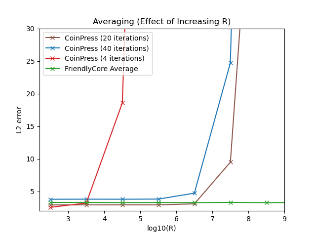
Refer to caption Refer to caption Refer to caption

Figure 5: From Left to Right: (1) Averaging in d=1000d=1000 and n=800n=800, varying RR. (2) Averaging in n=800n=800, R=10​dR=10\sqrt{d}, varying dd. (3) Averaging in d=50d=50 and R=10​dR=10\sqrt{d}, varying nn.

6.2 Clustering

We tested the performance of our private clustering algorithm 𝖥𝖢​_​𝖢𝗅𝗎𝗌𝗍𝖾𝗋𝗂𝗇𝗀\mathsf{FC\_Clustering} with t=200t=200 tuples on a number of kk-Means and kk-GMM tasks. We compared a Python implementation of 𝖥𝖢​_​𝖢𝗅𝗎𝗌𝗍𝖾𝗋𝗂𝗇𝗀\mathsf{FC\_Clustering} with a recent algorithm of [CK21] that is based on recursive locality-sensitive hashing (LSH). We denote their algorithm by 𝖫𝖲𝖧​_​𝖢𝗅𝗎𝗌𝗍𝖾𝗋𝗂𝗇𝗀\mathsf{LSH\_Clustering}. The implementations of 𝖫𝖲𝖧​_​𝖢𝗅𝗎𝗌𝗍𝖾𝗋𝗂𝗇𝗀\mathsf{LSH\_Clustering}, and the experimental test bed of Figure 6, were taken from the publicly available code of [CK21] provided at https://github.com/google/differential-privacy/tree/main/learning/clustering. 𝖫𝖲𝖧​_​𝖢𝗅𝗎𝗌𝗍𝖾𝗋𝗂𝗇𝗀\mathsf{LSH\_Clustering} guarantees privacy in the 𝖣𝖯{\sf DP} model. Therefore, in order to compare it with our (ρ=1,δ)(\rho=1,\delta)-𝗓𝖢𝖣𝖯{\sf zCDP} guarantee, we chose to apply it with a (ε=2,δ)(\varepsilon=2,\delta)-𝖣𝖯{\sf DP} guarantee, so that neither guarantee implies the other. Furthermore, unlike 𝖥𝖢​_​𝖢𝗅𝗎𝗌𝗍𝖾𝗋𝗂𝗇𝗀\mathsf{FC\_Clustering} which may fail to produce centers in some cases (e.g., when the core of tuples is empty or close to be empty), 𝖫𝖲𝖧​_​𝖢𝗅𝗎𝗌𝗍𝖾𝗋𝗂𝗇𝗀\mathsf{LSH\_Clustering} always produces centers. Therefore, in order to handle failures of 𝖥𝖢​_​𝖢𝗅𝗎𝗌𝗍𝖾𝗋𝗂𝗇𝗀\mathsf{FC\_Clustering}, we used only ρ=0.99\rho=0.99 privacy budget, and on failures we executed 𝖫𝖲𝖧​_​𝖢𝗅𝗎𝗌𝗍𝖾𝗋𝗂𝗇𝗀\mathsf{LSH\_Clustering} with ε=0.02\varepsilon=\sqrt{0.02} (which implies ρ=0.01\rho=0.01 𝗓𝖢𝖣𝖯{\sf zCDP}) as backup.

We performed 3030 repetitions of each experiment and present the medians (points) along with the 0.10.1 and 0.90.9 quantiles.

In Figure 6 (Left) we present a comparison in dimension d=2d=2 with k=8k=8 clusters. In each repetition, we sampled eight random centers {𝒄i}i=18\{\boldsymbol{c}_{i}\}_{i=1}^{8} from the unit ball, and the database was obtained by collecting n/8n/8 samples from each Gaussian 𝒩⁡(𝒄i, 0.0221​I2×2){\cal N}(\boldsymbol{c}_{i},\>0.0221I_{2\times 2}), where the samples were clipped to ℓ2\ell_{2} norm of 11. For 𝖥𝖢​_​𝖢𝗅𝗎𝗌𝗍𝖾𝗋𝗂𝗇𝗀\mathsf{FC\_Clustering} we used an oracle access to kk-means+⁣+++ provided by the KMeans algorithm of the Python library sklearn, and used rmin=0.001r_{\min}=0.001 and radius Λ=1\Lambda=1. We set the radius parameter of 𝖫𝖲𝖧​_​𝖢𝗅𝗎𝗌𝗍𝖾𝗋𝗂𝗇𝗀\mathsf{LSH\_Clustering} to 11. We plotted the normalized kk-means loss that is computed by 1−X/Y1-X/Y, where XX is the cost of kk-means+⁣+++ on the entire data, and YY is the cost of the tested private algorithm. From this experiment we observed that for small values of nn, 𝖥𝖢​_​𝖢𝗅𝗎𝗌𝗍𝖾𝗋𝗂𝗇𝗀\mathsf{FC\_Clustering} fails often, which yields inaccurate results. Yet, increasing nn also increases the success probability of 𝖥𝖢​_​𝖢𝗅𝗎𝗌𝗍𝖾𝗋𝗂𝗇𝗀\mathsf{FC\_Clustering} which yields very accurate results, while 𝖫𝖲𝖧​_​𝖢𝗅𝗎𝗌𝗍𝖾𝗋𝗂𝗇𝗀\mathsf{LSH\_Clustering} stay behind. See Figure 6 (Right) for a graphical illustration of the centers in one of the iterations for n=2⋅105n=2\cdot 10^{5}.

In Figure 7 (Left) we present a comparison for separating n=2.5⋅105n=2.5\cdot 10^{5} samples from a uniform mixture of k=5k=5 Gaussians 𝒩⁡(𝒄i,Id×d){\cal N}(\boldsymbol{c}_{i},\>I_{d\times d}) for varying dd. In each repetition, each of the 𝒄i\boldsymbol{c}_{i}’s was chosen uniformly from {1,2}d\{1,2\}^{d}, yielding that the distance between each pair of centers is ≈d/2\approx\sqrt{d/2}. We analyze the labeling accuracy, which is computed by finding the best permutation that fits between the true labeling and the induced clustering, and plotted the labeling failure of the best fit. Here, we used rmin=0.1r_{\min}=0.1, and radius Λ=10​d\Lambda=10\sqrt{d} for 𝖥𝖢​_​𝖢𝗅𝗎𝗌𝗍𝖾𝗋𝗂𝗇𝗀\mathsf{FC\_Clustering} and 𝖫𝖲𝖧​_​𝖢𝗅𝗎𝗌𝗍𝖾𝗋𝗂𝗇𝗀\mathsf{LSH\_Clustering}. For the non-private oracle access of 𝖥𝖢​_​𝖢𝗅𝗎𝗌𝗍𝖾𝗋𝗂𝗇𝗀\mathsf{FC\_Clustering}, we used a PCA-based clustering that easily separate between such Gaussians in high dimension.55 5 The algorithm project the points into the kk principal components, cluster the points in that low dimension, and then translate the clustering back to the original points and perform a Lloyd step. From this experiment we observed that 𝖥𝖢​_​𝖢𝗅𝗎𝗌𝗍𝖾𝗋𝗂𝗇𝗀\mathsf{FC\_Clustering} takes advantage of the PCA method and gains perfect accuracy on large values of dd, in contrast to 𝖫𝖲𝖧​_​𝖢𝗅𝗎𝗌𝗍𝖾𝗋𝗂𝗇𝗀\mathsf{LSH\_Clustering}.

At that point, we showed that 𝖥𝖢​_​𝖢𝗅𝗎𝗌𝗍𝖾𝗋𝗂𝗇𝗀\mathsf{FC\_Clustering} succeed well on well-separated databases, since the results of the non-private algorithm (each is executed on a random piece of data) are very similar to each other in such cases. We next show that such stability can also be achieved on large enough real-world datasets, even when there is no clear separation into kk clusters.

In Figure 7 (Right) we used the publicly available dataset of [FH15] that contains the acquired time series from 16 chemical gas sensors exposed to gas mixtures at varying concentration levels. The dataset contains ≈8​M\approx 8M rows, where each row contains 16 sensors’ measurements at a given point in time, so we translate each such row into a 1616-dimensional point. We compared the clustering algorithms for varying kk, where we used rmin=0.1r_{\min}=0.1, and radius Λ=105\Lambda=10^{5} for 𝖥𝖢​_​𝖢𝗅𝗎𝗌𝗍𝖾𝗋𝗂𝗇𝗀\mathsf{FC\_Clustering} and 𝖫𝖲𝖧​_​𝖢𝗅𝗎𝗌𝗍𝖾𝗋𝗂𝗇𝗀\mathsf{LSH\_Clustering}. We observed that 𝖥𝖢​_​𝖢𝗅𝗎𝗌𝗍𝖾𝗋𝗂𝗇𝗀\mathsf{FC\_Clustering}, with kk-means++ as the non-private oracle, succeed well on various kk’s, except of k=5k=5 in which it fails due to instability of the non-private algorithm.66 6 There are two different solutions for k=5k=5 that have similar low cost but do not match, yielding that when splitting the data into random pieces, the non-private KMeans choose one of them in one set of part and the other one in the other pieces, and therefore fails.

Refer to caption Refer to caption

Figure 6: Left: kk-means results in d=2d=2 and k=8k=8, for varying nn. Right: A graphical illustration of the centers in one of the iterations for n=2⋅105n=2\cdot 10^{5}. Green points are the centers of 𝖥𝖢​_​𝖢𝗅𝗎𝗌𝗍𝖾𝗋𝗂𝗇𝗀\mathsf{FC\_Clustering} and the red points are the centers of 𝖫𝖲𝖧​_​𝖢𝗅𝗎𝗌𝗍𝖾𝗋𝗂𝗇𝗀\mathsf{LSH\_Clustering}.

Refer to caption Refer to caption

Figure 7: Left: Labeling Failure of samples from a uniform mixture of k=5k=5 Gaussians, varying dd. Right: kk-means results on Gas Sensors’ measurements over time, varying kk.

In summary, we observed from the experiments that when 𝖥𝖢​_​𝖢𝗅𝗎𝗌𝗍𝖾𝗋𝗂𝗇𝗀\mathsf{FC\_Clustering} succeed, it outputs very accurate results. However, 𝖥𝖢​_​𝖢𝗅𝗎𝗌𝗍𝖾𝗋𝗂𝗇𝗀\mathsf{FC\_Clustering} may fail due to instability of the non-private algorithm on random pieces of the database. Hence, it seems that in cases where we have a clear separation or many points, we might gain by combining between 𝖥𝖢​_​𝖢𝗅𝗎𝗌𝗍𝖾𝗋𝗂𝗇𝗀\mathsf{FC\_Clustering} and 𝖫𝖲𝖧​_​𝖢𝗅𝗎𝗌𝗍𝖾𝗋𝗂𝗇𝗀\mathsf{LSH\_Clustering}. In this work we chose to spend 0.990.99 of the privacy budget on 𝖥𝖢​_​𝖢𝗅𝗎𝗌𝗍𝖾𝗋𝗂𝗇𝗀\mathsf{FC\_Clustering}, but other combinations might perform better on different cases.

7 Conclusion

We presented a general tool 𝖥𝗋𝗂𝖾𝗇𝖽𝗅𝗒𝖢𝗈𝗋𝖾\mathsf{FriendlyCore} for preprocessing metric data before privately aggregating it. The processed data is guaranteed to have some properties that can simplify or boost the accuracy of aggregation. Our tool is flexible, and in this work we illustrate it by presenting three different applications (averaging, clustering, and learning an unrestricted covariance matrix). We show the wide applicability of our framework by applying it to private mean estimation and clustering, and comparing it to private algorithms which are specifically tailored for those tasks. For private averaging, we presented a simple algorithm with dimension-independent preprocessing, that is also independent of the ℓ2\ell_{2} norm of the points.77 7 The latter property results with an optimal asymptotic that matches the histogram-based construction of [KV18] For private clustering, we presented the first practical algorithm that is based on the sample and aggregate framework of [NRS07], which has proven utility guarantees for easy instances (see Section C.3), and achieves very accurate results in practice when the data is either well separated or very large.

Acknowledgments

Edith Cohen is supported by Israel Science Foundation grant no. 1595-19.

Haim Kaplan is supported by Israel Science Foundation grant no. 1595-19, and the Blavatnik Family Foundation.

Yishay Mansour has received funding from the European Research Council (ERC) under the European Union’sHorizon 2020 research and innovation program (grant agreement No. 882396), by the Israel Science Foundation (grant number 993/17) and the Yandex Initiative for Machine Learning at Tel Aviv University.

Uri Stemmer is partially supported by the Israel Science Foundation (grant 1871/19) and by Len Blavatnik and the Blavatnik Family foundation.

References

  • [AL21] Hassan Ashtiani and Christopher Liaw “Private and polynomial time algorithms for learning Gaussians and beyond” In CoRR abs/2111.11320, 2021 arXiv: https://arxiv.org/abs/2111.11320
  • [AM05] Dimitris Achlioptas and Frank McSherry “On Spectral Learning of Mixtures of Distributions” In Learning Theory, 18th Annual Conference on Learning Theory, COLT 2005 3559, 2005, pp. 458–469
  • [BDKU20] Sourav Biswas, Yihe Dong, Gautam Kamath and Jonathan. Ullman “CoinPress: Practical Private Mean and Covariance Estimation” In Advances in Neural Information Processing Systems 33: Annual Conference on Neural Information Processing Systems, NeurIPS 2020, 2020
  • [BS16] Mark Bun and Thomas Steinke “Concentrated Differential Privacy: Simplifications, Extensions, and Lower Bounds” In Theory of Cryptography - 14th International Conference, TCC 2016 9985, 2016, pp. 635–658
  • [CK21] Alisa Chang and Pritish Kamath “Practical Differentially Private Clustering” In Google AI Blog, 2021 URL: https://ai.googleblog.com/2021/10/practical-differentially-private.htverbml
  • [CKM+21] Edith Cohen et al. “Differentially-Private Clustering of Easy Instances” In Proceedings of the 38th International Conference on Machine Learning, ICML 2021 139, 2021, pp. 2049–2059 URL: https://arxiv.org/abs/2112.14445
  • [DKM+06] Cynthia Dwork et al. “Our Data, Ourselves: Privacy Via Distributed Noise Generation” In EUROCRYPT 4004, 2006, pp. 486–503
  • [DL09] Cynthia Dwork and Jing Lei “Differential privacy and robust statistics” In STOC ACM, 2009, pp. 371–380
  • [DMNS06] Cynthia Dwork, Frank McSherry, Kobbi Nissim and Adam Smith “Calibrating Noise to Sensitivity in Private Data Analysis” In TCC 3876, 2006, pp. 265–284
  • [DRV10] Cynthia Dwork, Guy. Rothblum and Salil. Vadhan “Boosting and Differential Privacy” In FOCS IEEE Computer Society, 2010, pp. 51–60
  • [FH15] Jordi Fonollosa and Ramon Huerta “Reservoir Computing compensates slow response of chemosensor arrays exposed to fast varying gas concentrations in continuous monitoring” In Sensors and Actuators B, 2015 URL: http://archive.ics.uci.edu/ml/datasets/Gas+sensor+array+under+dynamicverb+gas+mixtures
  • [HLY21] Ziyue Huang, Yuting Liang and Ke Yi “Instance-optimal Mean Estimation Under Differential Privacy” In Advances in Neural Information Processing Systems 34, 2021, pp. 25993–26004
  • [KLSU19] Gautam Kamath, Jerry Li, Vikrant Singhal and Jonathan Ullman “Privately Learning High-Dimensional Distributions” In Conference on Learning Theory, COLT 2019, 25-28 June 2019, Phoenix, AZ, USA 99, Proceedings of Machine Learning Research PMLR, 2019, pp. 1853–1902
  • [KMS+21] Gautam Kamath et al. “A private and computationally-efficient estimator for unbounded gaussians” In CoRR abs/2111.04609, 2021 arXiv: https://arxiv.org/abs/2111.04609
  • [KMV21] Pravesh Kothari, Pasin Manurangsi and Ameya Velingker “Private Robust Estimation by Stabilizing Convex Relaxations” In CoRR abs/2112.03548, 2021 arXiv: https://arxiv.org/abs/2112.03548
  • [KNRS13] Shiva Kasiviswanathan, Kobbi Nissim, Sofya Raskhodnikova and Adam. Smith “Analyzing Graphs with Node Differential Privacy” In Theory of Cryptography - 10th Theory of Cryptography Conference, TCC 2013 7785, 2013, pp. 457–476
  • [KSSU19] Gautam Kamath, Or Sheffet, Vikrant Singhal and Jonathan Ullman “Differentially Private Algorithms for Learning Mixtures of Separated Gaussians” In Advances in Neural Information Processing Systems 32: Annual Conference on Neural Information Processing Systems, NeurIPS 2019, 2019, pp. 168–180
  • [KSU20] Gautam Kamath, Vikrant Singhal and Jonathan Ullman “Private mean estimation of heavy-tailed distributions” In arXiv preprint arXiv:2002.09464, 2020
  • [KV18] Vishesh Karwa and Salil Vadhan “Finite Sample Differentially Private Confidence Intervals” In 9th Innovations in Theoretical Computer Science Conference (ITCS 2018), 2018
  • [LSA+21] Daniel Levy et al. “Learning with User-Level Privacy” In Advances in Neural Information Processing Systems 34: Annual Conference on Neural Information Processing Systems 2021, NeurIPS 2021, 2021, pp. 12466–12479
  • [NRS07] Kobbi Nissim, Sofya Raskhodnikova and Adam Smith “Smooth sensitivity and sampling in private data analysis” In STOC ACM, 2007, pp. 75–84
  • [NSV16] Kobbi Nissim, Uri Stemmer and Salil. Vadhan “Locating a Small Cluster Privately” In Proceedings of the 35th ACM SIGMOD-SIGACT-SIGAI Symposium on Principles of Database Systems, PODS 2016, 2016, pp. 413–427
  • [ORSS12] Rafail Ostrovsky, Yuval Rabani, Leonard. Schulman and Chaitanya Swamy “The effectiveness of lloyd-type methods for the k-means problem” In J. ACM 59.6, 2012, pp. 28:1–28:22
  • [R“’61] Alfr“’ed R“’enyi “On measures of entropy and information” In Proceedings of the Fourth Berkeley Symposium on Mathematical Statistics and Probability, Volume 1: Contributions to the Theory of Statistics, 1961, pp. 547–561
  • [Sca09] M Scala “Hypergeometric tail inequalities: ending the insanity” In arXiv preprint arXiv:1311.5939, 2009
  • [She21] Moshe Shechner “Differentially private algorithms for clustering with stability assumptions”, 2021
  • [SS21] Vikrant Singhal and Thomas Steinke “Privately learning subspaces” In Advances in Neural Information Processing Systems 34, 2021
  • [SSS20] Moshe Shechner, Or Sheffet and Uri Stemmer “Private k-Means Clustering with Stability Assumptions” In The 23rd International Conference on Artificial Intelligence and Statistics, AISTATS 2020 108, Proceedings of Machine Learning Research, 2020, pp. 2518–2528

Appendix A Learning a Covariance Matrix

In this section, we are given a database that consists of independent samples from a Gaussian 𝒩⁡(0,Σ){\cal N}(0,\Sigma) where the covariance matrix Σ⪰0\Sigma\succeq 0 is unknown, no bounds on ‖Σ‖\mathopen{}\mathclose{{\left\lVert\Sigma}}\right\rVert (the operator norm) are given, and the goal is to privately estimate Σ\Sigma. Without privacy, it can just be estimated by the empirical covariance of the samples: 1n​∑i=1n𝒙i⋅𝒙iT\frac{1}{n}\sum_{i=1}^{n}\boldsymbol{x}_{i}\cdot\boldsymbol{x}_{i}^{T}. Recently, three independent and concurrent works of [KMS+21, AL21, KMV21] gave a polynomial-time algorithm for this problem (all the three works were published after the first version of our work that did not include the covariance matrix application). The core of [AL21]’s construction consists of a framework in the 𝖣𝖯{\sf DP} model for privately learning average-based aggregation tasks, that has the same flavor of 𝖥𝗋𝗂𝖾𝗇𝖽𝗅𝗒𝖢𝗈𝗋𝖾\mathsf{FriendlyCore}. Their tool does not output a subset 𝒞⊆𝒟{\cal C}\subseteq{\cal D} as 𝖥𝗋𝗂𝖾𝗇𝖽𝗅𝗒𝖢𝗈𝗋𝖾\mathsf{FriendlyCore}. Rather, it outputs a weighted average of the elements, where the weights are chosen in a way that makes the task of privately estimating it to be simpler than its unrestricted counterpart (in particular, their framework guarantees that “outliers” receive weight 00, and by that it is certified that the weighted average has only low sensitivity).88 8 The framework of [AL21] has similar ideas to 𝖥𝗋𝗂𝖾𝗇𝖽𝗅𝗒𝖢𝗈𝗋𝖾\mathsf{FriendlyCore}. However, it is wrapped by a more complicated abstraction, and it is not clear how to apply it for tasks like kk-tuple clustering, in which a weighted average is not meaningful. We therefore believe that 𝖥𝗋𝗂𝖾𝗇𝖽𝗅𝗒𝖢𝗈𝗋𝖾\mathsf{FriendlyCore}, apart of being practical, is also simpler, more intuitive and more general. For learning a covariance matrix, they implicitly use a special “friendliness” predicate between covariance matrices, and apply their tool on the empirical covariance matrices, each is computed (non-privately) from a different part of the data points.

We next show how to apply 𝖥𝗋𝗂𝖾𝗇𝖽𝗅𝗒𝖢𝗈𝗋𝖾\mathsf{FriendlyCore} along with the tools of [AL21] in order to privately learn an unrestricted covariance matrix. Similarly to [AL21], we only handle the case that Σ≻0\Sigma\succ 0 (i.e., where Σ\Sigma has full rank).99 9 The general case can be done by first privately computing the exact subspace using propose-test-release or a private histogram (see [SS21, AL21]), and then working on the resulting subspace with a full rank matrix. In addition, following the main step of [AL21], we only show the reduction to the restricted covariance case that is well studied (e.g., see [BDKU20, KLSU19]).

We start by defining a predicate and stating key properties from [AL21].

Definition A.1 (Predicate 𝗆𝖺𝗍𝗋𝗂𝗑𝖣𝗂𝗌𝗍γ{\sf matrixDist}_{\gamma} [AL21]).

For d×dd\times d matrices Σ1,Σ2⪰0\Sigma_{1},\Sigma_{2}\succeq 0, let

𝗆𝖺𝗍𝗋𝗂𝗑𝖣𝗂𝗌𝗍⁡(Σ1,Σ2):={OPENmax⁡(‖Σ2−1/2Σ1Σ2−1/2−Id‖,‖Σ1−1/2Σ2Σ1−1/2−Id‖)Σ1,Σ2≻0∞otherwise,\displaystyle{\sf matrixDist}(\Sigma_{1},\Sigma_{2}):=\begin{cases}\max\mathopen{}\mathclose{{\left(\mathopen{}\mathclose{{\left\lVert\Sigma_{2}^{-1/2}\Sigma_{1}\Sigma_{2}^{-1/2}-I_{d}}}\right\rVert,\mathopen{}\mathclose{{\left\lVert\Sigma_{1}^{-1/2}\Sigma_{2}\Sigma_{1}^{-1/2}-I_{d}}}\right\rVert}}\right)&\Sigma_{1},\Sigma_{2}\succ 0\\ \infty&\text{otherwise}\end{cases},

and for γ≥0\gamma\geq 0 let 𝗆𝖺𝗍𝗋𝗂𝗑𝖣𝗂𝗌𝗍γ(Σ1,Σ2):=𝟙{𝗆𝖺𝗍𝗋𝗂𝗑𝖣𝗂𝗌𝗍(Σ1,Σ2)≤γ}{\sf matrixDist}_{\gamma}(\Sigma_{1},\Sigma_{2}):=\mathds{1}_{\{{\sf matrixDist}(\Sigma_{1},\Sigma_{2})\leq\gamma\}}.

The intuition behind the distance measure 𝗆𝖺𝗍𝗋𝗂𝗑𝖣𝗂𝗌𝗍{\sf matrixDist} is that it does not scale with the norms of the matrices, i.e., 𝗆𝖺𝗍𝗋𝗂𝗑𝖣𝗂𝗌𝗍⁡(Σ1,Σ2)=𝗆𝖺𝗍𝗋𝗂𝗑𝖣𝗂𝗌𝗍⁡(λ​Σ1,λ​Σ2){\sf matrixDist}(\Sigma_{1},\Sigma_{2})={\sf matrixDist}(\lambda\Sigma_{1},\lambda\Sigma_{2}) for any λ>0\lambda>0. Therefore, it is useful in our case where we do not have any bounds on the norm of the covariance matrix.

In addition, 𝗆𝖺𝗍𝗋𝗂𝗑𝖣𝗂𝗌𝗍{\sf matrixDist} satisfies an approximate triangle inequality (stated bellow).

Lemma A.2 (Approximate triangle inequality (Lemma 7.2 in [AL21])).

If 𝗆𝖺𝗍𝗋𝗂𝗑𝖣𝗂𝗌𝗍⁡(Σ1,Σ2)≤1{\sf matrixDist}(\Sigma_{1},\Sigma_{2})\leq 1 and 𝗆𝖺𝗍𝗋𝗂𝗑𝖣𝗂𝗌𝗍⁡(Σ2,Σ3)≤1{\sf matrixDist}(\Sigma_{2},\Sigma_{3})\leq 1 then 𝑂𝑃𝐸𝑁𝗆𝖺𝗍𝗋𝗂𝗑𝖣𝗂𝗌𝗍⁡(Σ1,Σ3)≤32⋅(𝗆𝖺𝗍𝗋𝗂𝗑𝖣𝗂𝗌𝗍⁡(Σ1,Σ2)+𝗆𝖺𝗍𝗋𝗂𝗑𝖣𝗂𝗌𝗍⁡(Σ2,Σ3)𝐶𝐿𝑂𝑆𝐸){\sf matrixDist}(\Sigma_{1},\Sigma_{3})\leq\frac{3}{2}\cdot\mathopen{}\mathclose{{\left({\sf matrixDist}(\Sigma_{1},\Sigma_{2})+{\sf matrixDist}(\Sigma_{2},\Sigma_{3})}}\right).

Note that Appendix A implies that if 𝒟{\cal D} is 𝗆𝖺𝗍𝗋𝗂𝗑𝖣𝗂𝗌𝗍γ{\sf matrixDist}_{\gamma}-friendly (for γ≤1\gamma\leq 1), then it is 𝗆𝖺𝗍𝗋𝗂𝗑𝖣𝗂𝗌𝗍3​γ{\sf matrixDist}_{3\gamma}-complete.

The idea now is to apply 𝖥𝗋𝗂𝖾𝗇𝖽𝗅𝗒𝖢𝗈𝗋𝖾𝖣𝖯\mathsf{FriendlyCoreDP} with this predicate (using a small constant γ\gamma, say 0.10.1) in order to privately estimate the covariance matrix. At the high-level, this is done by the following process: (1) Split the samples into equal-size parts and compute the empirical covariance matrix of each part. (2) On the resulting database of matrices 𝒯=(Σ1,…,Σt){\cal T}=(\Sigma_{1},\ldots,\Sigma_{t}), apply 𝖥𝗋𝗂𝖾𝗇𝖽𝗅𝗒𝖢𝗈𝗋𝖾𝖣𝖯\mathsf{FriendlyCoreDP} for obtaining a core 𝒞⊆𝒯{\cal C}\subseteq{\cal T} that is certified to be 𝗆𝖺𝗍𝗋𝗂𝗑𝖣𝗂𝗌𝗍0.1{\sf matrixDist}_{0.1}-friendly. Then, execute an 𝗆𝖺𝗍𝗋𝗂𝗑𝖣𝗂𝗌𝗍0.1{\sf matrixDist}_{0.1}-friendly 𝖣𝖯{\sf DP} algorithm over the core 𝒞{\cal C}.

It is left to design an 𝗆𝖺𝗍𝗋𝗂𝗑𝖣𝗂𝗌𝗍0.1{\sf matrixDist}_{0.1}-friendly 𝖣𝖯{\sf DP} algorithm. The first step is to use the following fact which states that if 𝒯∪𝒯′{\cal T}\cup{\cal T}^{\prime} is 𝗆𝖺𝗍𝗋𝗂𝗑𝖣𝗂𝗌𝗍0.1{\sf matrixDist}_{0.1}-friendly (and therefore, 𝗆𝖺𝗍𝗋𝗂𝗑𝖣𝗂𝗌𝗍0.3{\sf matrixDist}_{0.3}-complete), then 𝗆𝖺𝗍𝗋𝗂𝗑𝖣𝗂𝗌𝗍(Avg(𝒯),Avg(𝒯′))≤O(1/|𝒯|){\sf matrixDist}({\rm Avg}({\cal T}),{\rm Avg}({\cal T}^{\prime}))\leq O(1/\mathopen{}\mathclose{{\left|{\cal T}}}\right|).

Lemma A.3 (Implicit in [AL21]).

There exists a constant c1>0c_{1}>0 such that the following holds: Let γ>0\gamma>0 and let Σ1,…,Σn≻0\Sigma_{1},\ldots,\Sigma_{n}\succ 0 such that 𝗆𝖺𝗍𝗋𝗂𝗑𝖣𝗂𝗌𝗍⁡(Σi,Σj)≤0.3{\sf matrixDist}(\Sigma_{i},\Sigma_{j})\leq 0.3 for every i,j∈[n]i,j\in[n]. Assuming that n≥c1/γn\geq c_{1}/\gamma, then it holds that 𝗆𝖺𝗍𝗋𝗂𝗑𝖣𝗂𝗌𝗍⁡(1n​∑i=1nΣi,1n−1​∑i=2nΣi)≤γ{\sf matrixDist}(\frac{1}{n}\sum_{i=1}^{n}\Sigma_{i},\>\frac{1}{n-1}\sum_{i=2}^{n}\Sigma_{i})\leq\gamma.

Next, we define a mechanism 𝖡η\mathsf{B}_{\eta} such that for any two matrices Σ1,Σ2\Sigma_{1},\Sigma_{2} with OPEN𝗆𝖺𝗍𝗋𝗂𝗑𝖣𝗂𝗌𝗍⁡(Σ1,Σ2)≤O~​(ε​ηd​ln⁡(2/δ)CLOSE){\sf matrixDist}(\Sigma_{1},\Sigma_{2})\leq\widetilde{O}\mathopen{}\mathclose{{\left(\frac{\varepsilon\eta}{\sqrt{d\ln(2/\delta)}}}}\right), it holds that 𝖡η(Σ1)≈ε,δ𝖣𝖯𝖡η(Σ2)\mathsf{B}_{\eta}(\Sigma_{1})\approx_{\varepsilon,\delta}^{{\sf DP}}\mathsf{B}_{\eta}(\Sigma_{2}).

Lemma A.4 (Lemma 9.1 in [AL21]).

For a matrix Σ≻0\Sigma\succ 0 and η>0\eta>0, define 𝖡η​(Σ):=Σ1/2​(I+η​G)​(I+η​G)T​Σ1/2\mathsf{B}_{\eta}(\Sigma):=\Sigma^{1/2}(I+\eta G)(I+\eta G)^{T}\Sigma^{1/2}, where GG is a d×dd\times d matrix with independent 𝒩⁡(0,1){\cal N}(0,1) entries. Then for every η>0\eta>0, ε,δ∈(0,1]\varepsilon,\delta\in(0,1], and every matrices Σ1,Σ2≻0\Sigma_{1},\Sigma_{2}\succ 0 such that 𝗆𝖺𝗍𝗋𝗂𝗑𝖣𝗂𝗌𝗍⁡(Σ1,Σ2)≤γ{\sf matrixDist}(\Sigma_{1},\Sigma_{2})\leq\gamma for

γ=min⁡{ε2​d​(d+1/η2),ε8​d​ln⁡(1/δ),ε8​ln⁡(2/δ),ε​η12​d​ln⁡(2/δ)},\displaystyle\gamma=\min\{\sqrt{\frac{\varepsilon}{2d(d+1/\eta^{2})}},\frac{\varepsilon}{8d\sqrt{\ln(1/\delta)}},\frac{\varepsilon}{8\ln(2/\delta)},\frac{\varepsilon\eta}{12\sqrt{d\ln(2/\delta)}}\},

it holds that 𝖡η(Σ1)≈ε,δ𝖣𝖯𝖡η(Σ2)\mathsf{B}_{\eta}(\Sigma_{1})\approx_{\varepsilon,\delta}^{{\sf DP}}\mathsf{B}_{\eta}(\Sigma_{2}).

We now describe our friendly 𝖣𝖯{\sf DP} algorithm for estimating the mean of covariance matrices.

Algorithm A.5 (𝖥𝗋𝗂𝖾𝗇𝖽𝗅𝗒𝖢𝗈𝗏𝖺𝗋𝗂𝖺𝗇𝖼𝖾\mathsf{FriendlyCovariance}).
  • [1] Input: A database 𝒟=(Σ1,…,Σn)∈(ℝd×d)∗{\cal D}=(\Sigma_{1},\ldots,\Sigma_{n})\in({\mathbb{R}}^{d\times d})^{*} and parameters ε,δ,η>0\varepsilon,\delta,\eta>0.
  • [2] Operation:  1. Let n=|𝒟|n=\mathopen{}\mathclose{{\left|{\cal D}}}\right|, let ε1=0.1​ε\varepsilon_{1}=0.1\varepsilon and ε2=0.9​ε\varepsilon_{2}=0.9\varepsilon, let γ=γ⁡(η,ε2,δ​e−ε1)\gamma=\gamma(\eta,\varepsilon_{2},\delta e^{-\varepsilon_{1}}) be the value from Appendix A, and let c1c_{1} be the constant from Appendix A. 2. Compute n^=n−ln⁡(1/δ)ε1+Lap⁡(1/ε1)\hat{n}=n-\frac{\ln(1/\delta)}{\varepsilon_{1}}+{\rm Lap}(1/\varepsilon_{1}). 3. If n=0n=0 or n^≤c1/γ\hat{n}\leq c_{1}/\gamma, output ⟂\perp and abort. 4. Output OPEN𝖡η​(1n​∑i=1nΣiCLOSE)\mathsf{B}_{\eta}\mathopen{}\mathclose{{\left(\frac{1}{n}\sum_{i=1}^{n}\Sigma_{i}}}\right), where 𝖡η\mathsf{B}_{\eta} is the algorithm from Appendix A.
  • Claim A.6 (Privacy of 𝖥𝗋𝗂𝖾𝗇𝖽𝗅𝗒𝖢𝗈𝗏𝖺𝗋𝗂𝖺𝗇𝖼𝖾\mathsf{FriendlyCovariance}).

    Algorithm 𝖥𝗋𝗂𝖾𝗇𝖽𝗅𝗒𝖢𝗈𝗏𝖺𝗋𝗂𝖺𝗇𝖼𝖾⁡(⋅,ε,δ,γ)\mathsf{FriendlyCovariance}(\cdot,\varepsilon,\delta,\gamma) is 𝗆𝖺𝗍𝗋𝗂𝗑𝖣𝗂𝗌𝗍0.1{\sf matrixDist}_{0.1}-friendly (ε,δ)(\varepsilon,\delta)-𝖣𝖯{\sf DP}.

    For proving Appendix A we use the following simple fact.

    Fact A.7.

    Let X,X′X,X^{\prime} be two random variables over 𝒳{\cal X}. Assume there exist events E,E′⊆𝒳E,E^{\prime}\subseteq{\cal X} such that: (1) Pr[X∈E]∈e±ε1⋅Pr[X′∈E′]{\mathrm{Pr}}\mathopen{}\mathclose{{\left[X\in E}}\right]\in e^{\pm\varepsilon_{1}}\cdot{\mathrm{Pr}}\mathopen{}\mathclose{{\left[X^{\prime}\in E^{\prime}}}\right], and (2) X|E≈ε2,δ𝖣𝖯X′|E′X|_{E}\approx_{\varepsilon_{2},\delta}^{{\sf DP}}X^{\prime}|_{E^{\prime}}, and (3) X|¬E≈ε2,δ𝖣𝖯X′|¬E′X|_{\neg E}\approx_{\varepsilon_{2},\delta}^{{\sf DP}}X^{\prime}|_{\neg E^{\prime}}. Then X≈ε1+ε2,δ​eε1𝖣𝖯X′X\approx_{\varepsilon_{1}+\varepsilon_{2},\>\delta e^{\varepsilon_{1}}}^{{\sf DP}}X^{\prime}.

    Proof.

    Fix an event T⊆𝒳T\subseteq{\cal X} and compute

    Pr[X∈T]=Pr[X∈T∣E]⋅Pr[X∈E]+Pr[X∈T∣¬E]⋅Pr[X∉E]\displaystyle{\mathrm{Pr}}\mathopen{}\mathclose{{\left[X\in T}}\right]={\mathrm{Pr}}\mathopen{}\mathclose{{\left[X\in T\mid E}}\right]\cdot{\mathrm{Pr}}\mathopen{}\mathclose{{\left[X\in E}}\right]+{\mathrm{Pr}}\mathopen{}\mathclose{{\left[X\in T\mid\neg E}}\right]\cdot{\mathrm{Pr}}\mathopen{}\mathclose{{\left[X\notin E}}\right]
    ≤(eε2⋅Pr[X′∈T∣E′]+δ)⋅eε1⋅Pr[X′∈E′]+(eε2⋅Pr[X′∈T∣¬E′]+δ)⋅eε1⋅Pr[X′∉E′]\displaystyle\leq\mathopen{}\mathclose{{\left(e^{\varepsilon_{2}}\cdot{\mathrm{Pr}}\mathopen{}\mathclose{{\left[X^{\prime}\in T\mid E^{\prime}}}\right]+\delta}}\right)\cdot e^{\varepsilon_{1}}\cdot{\mathrm{Pr}}\mathopen{}\mathclose{{\left[X^{\prime}\in E^{\prime}}}\right]+\mathopen{}\mathclose{{\left(e^{\varepsilon_{2}}\cdot{\mathrm{Pr}}\mathopen{}\mathclose{{\left[X^{\prime}\in T\mid\neg E^{\prime}}}\right]+\delta}}\right)\cdot e^{\varepsilon_{1}}\cdot{\mathrm{Pr}}\mathopen{}\mathclose{{\left[X^{\prime}\notin E^{\prime}}}\right]
    =eε1+ε2⋅Pr[X′∈T]+δeε1.\displaystyle=e^{\varepsilon_{1}+\varepsilon_{2}}\cdot{\mathrm{Pr}}\mathopen{}\mathclose{{\left[X^{\prime}\in T}}\right]+\delta e^{\varepsilon_{1}}.

    □\Box

    We now prove Appendix A using Appendix A.

    Proof.

    Let 𝒟=(Σ1,…,Σn){\cal D}=(\Sigma_{1},\ldots,\Sigma_{n}) and 𝒟′=𝒟−j{\cal D}^{\prime}={\cal D}_{-j} be two 𝗆𝖺𝗍𝗋𝗂𝗑𝖣𝗂𝗌𝗍0.1{\sf matrixDist}_{0.1}-friendly neighboring databases, and let n′=n−1n^{\prime}=n-1. Consider two independent random executions of 𝖥𝗋𝗂𝖾𝗇𝖽𝗅𝗒𝖢𝗈𝗏𝖺𝗋𝗂𝖺𝗇𝖼𝖾⁡(𝒟)\mathsf{FriendlyCovariance}({\cal D}) and 𝖥𝗋𝗂𝖾𝗇𝖽𝗅𝗒𝖢𝗈𝗏𝖺𝗋𝗂𝖺𝗇𝖼𝖾⁡(𝒟′)\mathsf{FriendlyCovariance}({\cal D}^{\prime}) (both with the same input parameters ε,δ,η\varepsilon,\delta,\eta). Let N^\widehat{N} and OO be the (r.v.’s of the) values of n^\hat{n} and the output in the execution 𝖥𝗋𝗂𝖾𝗇𝖽𝗅𝗒𝖠𝗏𝗀⁡(𝒟)\mathsf{FriendlyAvg}({\cal D}), let N^′\widehat{N}^{\prime} and O′O^{\prime} be these r.v.’s w.r.t. the execution 𝖥𝗋𝗂𝖾𝗇𝖽𝗅𝗒𝖢𝗈𝗏𝖺𝗋𝗂𝖺𝗇𝖼𝖾⁡(𝒟′)\mathsf{FriendlyCovariance}({\cal D}^{\prime}), and let ε1,ε2\varepsilon_{1},\varepsilon_{2} be as in Step 1. If n≤c1/γn\leq c_{1}/\gamma then Pr[O=⟂],Pr[O′=⟂]≥1−δ{\mathrm{Pr}}\mathopen{}\mathclose{{\left[O=\perp}}\right],{\mathrm{Pr}}\mathopen{}\mathclose{{\left[O^{\prime}=\perp}}\right]\geq 1-\delta and we conclude that O≈0,δ𝖣𝖯O′O\approx_{0,\delta}^{{\sf DP}}O^{\prime} in this case.

    It is left to handle the case n≥c1/γn\geq c_{1}/\gamma. Let EE be the event {O≠⟂}\{O\neq\perp\} and E′E^{\prime} be the event {O′≠⟂}\{O^{\prime}\neq\perp\}. By construction it is clear that Pr[E]∈e±ε1Pr[E′]{\mathrm{Pr}}\mathopen{}\mathclose{{\left[E}}\right]\in e^{\pm\varepsilon_{1}}{\mathrm{Pr}}\mathopen{}\mathclose{{\left[E^{\prime}}}\right] and that O|¬E≡O|¬E′O|_{\neg E}\equiv O|_{\neg E^{\prime}} (under the conditioning on ¬E\neg E and ¬E′\neg E^{\prime}, it holds that O=O′=⟂O=O^{\prime}=\perp). By Appendix A, it suffices to prove that O|E≈ε2,δ​e−ε1𝖣𝖯O′|E′O|_{E}\approx_{\varepsilon_{2},\>\delta e^{-\varepsilon_{1}}}^{{\sf DP}}O^{\prime}|_{E^{\prime}} for showing that O≈ε,δ𝖣𝖯O′O\approx_{\varepsilon,\delta}^{{\sf DP}}O^{\prime}.

    Since 𝒟∪𝒟′{\cal D}\cup{\cal D}^{\prime} is 𝗆𝖺𝗍𝗋𝗂𝗑𝖣𝗂𝗌𝗍0.1{\sf matrixDist}_{0.1}-friendly, we deduce by approximate triangle inequality (Appendix A) that it is 𝗆𝖺𝗍𝗋𝗂𝗑𝖣𝗂𝗌𝗍0.3{\sf matrixDist}_{0.3}-complete. Let Σ=1n​∑i∈[n]Σi\Sigma=\frac{1}{n}\sum_{i\in[n]}\Sigma_{i} and Σ′=1n−1​∑i∈[n]∖{j}Σi\Sigma^{\prime}=\frac{1}{n-1}\sum_{i\in[n]\setminus\{j\}}\Sigma_{i}. By Appendix A it holds that 𝗆𝖺𝗍𝗋𝗂𝗑𝖣𝗂𝗌𝗍⁡(Σ,Σ′)≤γ{\sf matrixDist}(\Sigma,\Sigma^{\prime})\leq\gamma. Since O|E=𝖡η​(Σ)O|_{E}=\mathsf{B}_{\eta}(\Sigma) and O′|E′=𝖡η​(Σ′)O^{\prime}|_{E^{\prime}}=\mathsf{B}_{\eta}(\Sigma^{\prime}), we conclude by Appendix A that O|E≈ε2,δ​e−ε1𝖣𝖯O′|E′O|_{E}\approx_{\varepsilon_{2},\>\delta e^{-\varepsilon_{1}}}^{{\sf DP}}O^{\prime}|_{E^{\prime}}, as required.

    □\Box

    We now formally describe the end-to-end 𝖣𝖯{\sf DP} algorithm for covariance estimation:

    Algorithm A.8 (𝖥𝖢​_​𝖢𝗈𝗏𝖺𝗋𝗂𝖺𝗇𝖼𝖾\mathsf{FC\_Covariance}).
  • [3] Input: A database 𝒟=(𝒙1,…,𝒙n)∈(ℝd)∗{\cal D}=(\boldsymbol{x}_{1},\ldots,\boldsymbol{x}_{n})\in({\mathbb{R}}^{d})^{*}, privacy parameters ε,δ∈(0,1]\varepsilon,\delta\in(0,1], and parameters t∈ℕt\in{\mathbb{N}} and η>0\eta>0.
  • [4] Operation:  1. Let m=⌊n/t⌋m=\mathopen{}\mathclose{{\left\lfloor n/t}}\right\rfloor. 2. For i∈[t]i\in[t]: Compute Σi=1m⋅∑j=(i−1)⋅m+1i⋅m𝒙j⋅𝒙jT\Sigma_{i}=\frac{1}{m}\cdot\sum_{j=(i-1)\cdot m+1}^{i\cdot m}\boldsymbol{x}_{j}\cdot\boldsymbol{x}_{j}^{T}. 3. Let 𝒯=(Σ1,…,Σt){\cal T}=(\Sigma_{1},\ldots,\Sigma_{t}). 4. Compute 𝒞=𝖥𝗋𝗂𝖾𝗇𝖽𝗅𝗒𝖢𝗈𝗋𝖾𝖣𝖯⁡(𝒯,𝗆𝖺𝗍𝗋𝗂𝗑𝖣𝗂𝗌𝗍0.1,α=0){\cal C}=\mathsf{FriendlyCoreDP}({\cal T},{\sf matrixDist}_{0.1},\alpha=0). 5. Output 𝖥𝗋𝗂𝖾𝗇𝖽𝗅𝗒𝖢𝗈𝗏𝖺𝗋𝗂𝖺𝗇𝖼𝖾⁡(𝒞,ε,δ,η)\mathsf{FriendlyCovariance}({\cal C},\varepsilon,\delta,\eta).
  • Theorem A.9 (Privacy of 𝖥𝖢​_​𝖢𝗈𝗏𝖺𝗋𝗂𝖺𝗇𝖼𝖾\mathsf{FC\_Covariance}).

    𝖥𝖢​_​𝖢𝗈𝗏𝖺𝗋𝗂𝖺𝗇𝖼𝖾​(⋅,ε,δ,t)\mathsf{FC\_Covariance}(\cdot,\varepsilon,\delta,t) is (2​(eε−1),2​δ​eε+2​(eε−1))(2(e^{\varepsilon}-1),2\delta e^{\varepsilon+2(e^{\varepsilon}-1)})-𝖣𝖯{\sf DP}.

    Proof.

    Immediately follows by the privacy guarantee of 𝖥𝗋𝗂𝖾𝗇𝖽𝗅𝗒𝖢𝗈𝗋𝖾𝖣𝖯\mathsf{FriendlyCoreDP} (Theorem 4.11) because 𝖥𝗋𝗂𝖾𝗇𝖽𝗅𝗒𝖢𝗈𝗏𝖺𝗋𝗂𝖺𝗇𝖼𝖾\mathsf{FriendlyCovariance} is 𝗆𝖺𝗍𝗋𝗂𝗑𝖣𝗂𝗌𝗍0.1{\sf matrixDist}_{0.1}-friendly (ε,δ)(\varepsilon,\delta)-𝖣𝖯{\sf DP} (Appendix A).   □\Box

    A.1 Utility of 𝖥𝖢​_​𝖢𝗈𝗏𝖺𝗋𝗂𝖺𝗇𝖼𝖾\mathsf{FC\_Covariance}

    The following key lemma (Section A.1) implies that it is enough to take OPENn=Ω~​(t⋅(d+ln⁡(1/β))CLOSE)n=\tilde{\Omega}\mathopen{}\mathclose{{\left(t\cdot(d+\ln(1/\beta))}}\right) samples in order to guarantee with confidence 1−β/31-\beta/3 that the database 𝒯{\cal T} is 𝗆𝖺𝗍𝗋𝗂𝗑𝖣𝗂𝗌𝗍0.1{\sf matrixDist}_{0.1}-complete, yielding that 𝖥𝗋𝗂𝖾𝗇𝖽𝗅𝗒𝖢𝗈𝗋𝖾𝖣𝖯\mathsf{FriendlyCoreDP} takes all matrices into the core.

    Lemma A.10 (Lemma 9.3 in [AL21]).

    There exists a constant c2>0c_{2}>0 such that the following holds: Let m≥c2​(d+ln⁡(6/β))m\geq c_{2}(d+\ln(6/\beta)), let X1,…,XmX_{1},\ldots,X_{m} be i.i.d. samples from 𝒩⁡(0,Σ){\cal N}(0,\Sigma) for Σ≻0\Sigma\succ 0, and let Σ^=1m⋅∑i=1mXi​XiT\widehat{\Sigma}=\frac{1}{m}\cdot\sum_{i=1}^{m}X_{i}X_{i}^{T}. Then 𝗆𝖺𝗍𝗋𝗂𝗑𝖣𝗂𝗌𝗍⁡(Σ,Σ^)≤1/30{\sf matrixDist}(\Sigma,\widehat{\Sigma})\leq 1/30 with probability 1−β/31-\beta/3.

    In addition, [AL21] proved that choosing OPENη=Θ​(1d+ln⁡(1/β)CLOSE)\eta=\Theta\mathopen{}\mathclose{{\left(\frac{1}{\sqrt{d}+\sqrt{\ln(1/\beta)}}}}\right) suffices for making algorithm 𝖡η\mathsf{B}_{\eta} accurate, as stated below.

    Lemma A.11 (Lemma 9.2 in [AL21]).

    There exists a constant c3>0c_{3}>0 such that the following holds: Let η=1c3​(d+ln⁡(6/β))\eta=\frac{1}{c_{3}(\sqrt{d}+\sqrt{\ln(6/\beta)})} and let 𝖡η\mathsf{B}_{\eta} be the algorithm from Appendix A. Then for any Σ≻0\Sigma\succ 0 it holds that 𝗆𝖺𝗍𝗋𝗂𝗑𝖣𝗂𝗌𝗍⁡(𝖡η​(Σ),Σ)≤1/30{\sf matrixDist}(\mathsf{B}_{\eta}(\Sigma),\Sigma)\leq 1/30 with probability 1−β/31-\beta/3.

    Now note that by Step 3 of 𝖥𝗋𝗂𝖾𝗇𝖽𝗅𝗒𝖢𝗈𝗏𝖺𝗋𝗂𝖺𝗇𝖼𝖾\mathsf{FriendlyCovariance}, it is required to create at least OPENt=Ω​(1γ+ln⁡(1/(β​δ))εCLOSE)t=\Omega\mathopen{}\mathclose{{\left(\frac{1}{\gamma}+\frac{\ln(1/(\beta\delta))}{\varepsilon}}}\right) matrices in order to fail with probability at most β/3\beta/3.

    Putting all together, we obtain the following utility guarantee.

    Theorem A.12 (Utility of 𝖥𝖢​_​𝖢𝗈𝗏𝖺𝗋𝗂𝖺𝗇𝖼𝖾\mathsf{FC\_Covariance}).

    Let c1,c2c_{1},c_{2} and c3c_{3} be the constants from Appendices A, A.1 and A.1 (respectively), Let m=c2​(d+ln⁡(6/β))m=c_{2}(d+\ln(6/\beta)), let η=1c3​(d+ln⁡(6/β))\eta=\frac{1}{c_{3}(\sqrt{d}+\sqrt{\ln(6/\beta)})}, and let t=c1/γ+ln⁡(1/δ)+ln⁡(3/β)t=c_{1}/\gamma+\ln(1/\delta)+\ln(3/\beta) where 𝑂𝑃𝐸𝑁γ=γ⁡(η,0.9​ε,δ​e−0.1​ε)=O~​(εd​ln⁡(1/β)​ln⁡(1/δ)𝐶𝐿𝑂𝑆𝐸)\gamma=\gamma(\eta,0.9\varepsilon,\delta e^{-0.1\varepsilon})=\widetilde{O}\mathopen{}\mathclose{{\left(\frac{\varepsilon}{d\sqrt{\ln(1/\beta)\ln(1/\delta)}}}}\right) is the value from Appendix A. Consider a random execution of 𝖥𝖢​_​𝖢𝗈𝗏𝖺𝗋𝗂𝖺𝗇𝖼𝖾​(𝒟=(X1,…,Xn),ε,δ,t,η)\mathsf{FC\_Covariance}({\cal D}=(X_{1},\ldots,X_{n}),\varepsilon,\delta,t,\eta) where n=m⋅tn=m\cdot t and X1,…,XnX_{1},\ldots,X_{n} are i.i.d. samples from 𝒩⁡(0,Σ){\cal N}(0,\Sigma) for Σ≻0\Sigma\succ 0. Then with probability 1−β1-\beta, the output Σ^\widehat{\Sigma} satisfy 𝗆𝖺𝗍𝗋𝗂𝗑𝖣𝗂𝗌𝗍⁡(Σ^,Σ)≤0.1{\sf matrixDist}(\widehat{\Sigma},\Sigma)\leq 0.1.

    Note that the overall sample complexity that Theorem A.12 requires is OPENn=Ω~​(d2​ln⁡(1/β)3/2​ln​(1/δ)1/2εCLOSE)n=\widetilde{\Omega}\mathopen{}\mathclose{{\left(\frac{d^{2}\ln(1/\beta)^{3/2}\ln(1/\delta)^{1/2}}{\varepsilon}}}\right) which matches the sample complexity of [AL21] (Theorem 9.4).

    Proof.

    Let CC and T=(Σ1,…,Σt)T=(\Sigma_{1},\ldots,\Sigma_{t}) be the (r.v.’s of the) values of 𝒞{\cal C} and 𝒯{\cal T} in the execution. Let E1E_{1} be the event that ∀i∈[t]:𝗆𝖺𝗍𝗋𝗂𝗑𝖣𝗂𝗌𝗍⁡(Σi,Σ)≤1/30\forall i\in[t]:\>{\sf matrixDist}(\Sigma_{i},\Sigma)\leq 1/30, and let E2E_{2} be the event that 𝖥𝗋𝗂𝖾𝗇𝖽𝗅𝗒𝖢𝗈𝗏𝖺𝗋𝗂𝖺𝗇𝖼𝖾\mathsf{FriendlyCovariance} outputs a matrix Σ^\widehat{\Sigma} (and not ⟂\perp). By Section A.1 we obtain that Pr[E1]≥1−β/3{\mathrm{Pr}}\mathopen{}\mathclose{{\left[E_{1}}}\right]\geq 1-\beta/3, and in the following we assume it occurs. Note that by approximate triangle inequality (Appendix A) we obtain that TT is 𝗆𝖺𝗍𝗋𝗂𝗑𝖣𝗂𝗌𝗍0.1{\sf matrixDist}_{0.1}-complete, and therefore C=TC=T by the utility of 𝖥𝗋𝗂𝖾𝗇𝖽𝗅𝗒𝖢𝗈𝗋𝖾𝖣𝖯\mathsf{FriendlyCoreDP} (Theorem 4.11). By definition of tt (the size of CC in this case) and concentration bound of the Laplace distribution, it holds that Pr[E2∣E1]≥1−β/3{\mathrm{Pr}}\mathopen{}\mathclose{{\left[E_{2}\mid E_{1}}}\right]\geq 1-\beta/3, and in the following we assume it occurs. Let E3E_{3} be the event that the output Σ^\widehat{\Sigma} satisfy 𝗆𝖺𝗍𝗋𝗂𝗑𝖣𝗂𝗌𝗍⁡(Σ^,Avg⁡(T))≤1/30{\sf matrixDist}(\widehat{\Sigma},{\rm Avg}(T))\leq 1/30. By Section A.1 it holds that Pr[E3∣E1∧E2]≥1−β/3{\mathrm{Pr}}\mathopen{}\mathclose{{\left[E_{3}\mid E_{1}\land E_{2}}}\right]\geq 1-\beta/3, and in the following we assume it occurs. By the convexity of 𝗆𝖺𝗍𝗋𝗂𝗑𝖣𝗂𝗌𝗍{\sf matrixDist} (Lemma 7.2 in [AL21]), we deduce that 𝗆𝖺𝗍𝗋𝗂𝗑𝖣𝗂𝗌𝗍⁡(Avg⁡(T),Σ)≤1/30{\sf matrixDist}({\rm Avg}(T),\Sigma)\leq 1/30. Hence by applying again approximate triangle inequality (Appendix A) we conclude that 𝗆𝖺𝗍𝗋𝗂𝗑𝖣𝗂𝗌𝗍⁡(Σ^,Σ)≤0.1{\sf matrixDist}(\widehat{\Sigma},\Sigma)\leq 0.1 whenever E1∧E2∧E3E_{1}\land E_{2}\land E_{3} occurs, and the proof of the theorem follows since this event happens with probability 1−β1-\beta.   □\Box

    We note that by Theorem A.12, with probability 1−β1-\beta, 𝖥𝖢​_​𝖢𝗈𝗏𝖺𝗋𝗂𝖺𝗇𝖼𝖾\mathsf{FC\_Covariance} outputs a matrix Σ^\widehat{\Sigma} such that 0.9Id⪯Σ^−1/2ΣΣ^1/2⪯1.1Id0.9I_{d}\preceq\widehat{\Sigma}^{-1/2}\Sigma\widehat{\Sigma}^{1/2}\preceq 1.1I_{d}. In addition, note that if X∼𝒩⁡(0,Σ)X\sim{\cal N}(0,\Sigma), then Σ^−1/2X∼𝒩(0,Σ^−1/2ΣΣ^1/2)\widehat{\Sigma}^{-1/2}X\sim{\cal N}(0,\widehat{\Sigma}^{-1/2}\Sigma\widehat{\Sigma}^{1/2}). Therefore, we reduced the problem to the restricted covariance case.

    Appendix B Computational Efficiency of 𝖥𝗋𝗂𝖾𝗇𝖽𝗅𝗒𝖢𝗈𝗋𝖾\mathsf{FriendlyCore}

    Recall that our filters 𝖡𝖺𝗌𝗂𝖼𝖥𝗂𝗅𝗍𝖾𝗋\mathsf{BasicFilter} and 𝗓𝖢𝖣𝖯𝖥𝗂𝗅𝗍𝖾𝗋\mathsf{zCDPFilter} (the main components of 𝖥𝗋𝗂𝖾𝗇𝖽𝗅𝗒𝖢𝗈𝗋𝖾𝖣𝖯\mathsf{FriendlyCoreDP} and 𝖥𝗋𝗂𝖾𝗇𝖽𝗅𝗒𝖢𝗈𝗋𝖾\mathsf{FriendlyCore}, respectively) compute f⁡(x,y)f(x,y) for all pairs, that is, doing O⁡(n2)O(n^{2}) applications of the predicate. However, using standard concentration bounds, it is possible to use a random sample of O⁡(log⁡(n/δ))O(\log(n/\delta)) elements yy for estimating with high accuracy the number of friends of each xx.

    In more detail, given a database 𝒟=(x1,…,xn){\cal D}=(x_{1},\ldots,x_{n}), the goal is to efficiently estimate wi:=∑i=jnf⁡(xi,xj)w_{i}:=\sum_{i=j}^{n}f(x_{i},x_{j}) for each i∈[n]i\in[n]. For that, we can sample a random mm-size subset 𝒮=(y1,…,ym){\cal S}=(y_{1},\ldots,y_{m}) of 𝒟{\cal D} (without replacement). Then, we use the estimations w~i=nm⋅∑j=1mf⁡(xi,yj)\tilde{w}_{i}=\frac{n}{m}\cdot\sum_{j=1}^{m}f(x_{i},y_{j}). For making the privacy analysis go through, we need to replace each zi=wi−n/2z_{i}=w_{i}-n/2 with a value z~i\tilde{z}_{i} such that for all i∈[n]i\in[n], if zi≤0z_{i}\leq 0 then z~i≤0\tilde{z}_{i}\leq 0 (except with probability δ\delta). Note that if zi≤0z_{i}\leq 0 (i.e., wi≤n/2w_{i}\leq n/2), then ∑j=1mf⁡(xi,yj)\sum_{j=1}^{m}f(x_{i},y_{j}) (where the yjy_{j}’s are the random variables) is distributed according to the Hypergeometric distribution ℋ​𝒢​(n,wi,m)\mathcal{HG}(n,w_{i},m) which is defined by the number of ones in an mm-size random subset of an nn-size binary vector with wiw_{i} ones. We now use the following tail inequality for Hypergeometric distribution:

    Fact B.1 ([Sca09], Equation 10).

    Let SS be distributed according to ℋ​𝒢​(n,w,m)\mathcal{HG}(n,w,m). Then

    ∀ξ≥0:Pr[S≥(w/n+ξ)⋅m]≤e−2​ξ2​m\displaystyle\forall\xi\geq 0:\quad{\mathrm{Pr}}\mathopen{}\mathclose{{\left[S\geq(w/n+\xi)\cdot m}}\right]\leq e^{-2\xi^{2}m}

    By Appendix B, if wi≤n/2w_{i}\leq n/2 then Pr[w~i≥(1/2+ξ)n]≤e−2​ξ2​m{\mathrm{Pr}}\mathopen{}\mathclose{{\left[\tilde{w}_{i}\geq(1/2+\xi)n}}\right]\leq e^{-2\xi^{2}m}. By taking mm of the form m=12​ξ2⋅ln⁡(n/δ)m=\frac{1}{2\xi^{2}}\cdot\ln(n/\delta) we obtain that with probability 1−δ1-\delta, for every i∈[n]i\in[n] it holds that zi≤0⟹w~i≤(1/2+ξ)​nz_{i}\leq 0\implies\tilde{w}_{i}\leq(1/2+\xi)n. Therefore, the only change we should do is to replace the value zi=wi−n/2z_{i}=w_{i}-n/2 (computed in 𝖡𝖺𝗌𝗂𝖼𝖥𝗂𝗅𝗍𝖾𝗋\mathsf{BasicFilter} and 𝗓𝖢𝖣𝖯𝖥𝗂𝗅𝗍𝖾𝗋\mathsf{zCDPFilter}) with the value z~i:=w~i−(1/2+ξ)​n\tilde{z}_{i}:=\tilde{w}_{i}-(1/2+\xi)n. This results with a privacy guarantee that is equivalent to Theorems 4.8 and 4.11 up to an additional δ\delta in the privacy approximation error. Regarding utility guarantees, in Theorem 4.8 (𝗓𝖢𝖣𝖯{\sf zCDP} model), this change means that using the same lower bound on nn implies now a utility guarantee for elements with (1−α+ξ)​n(1-\alpha+\xi)n friends (rather than (1−α)​n(1-\alpha)n).1010 10 In the 𝖣𝖯{\sf DP} model we slightly need to change the probabilities pip_{i}’s in 𝖡𝖺𝗌𝗂𝖼𝖥𝗂𝗅𝗍𝖾𝗋\mathsf{BasicFilter} such that z~i≥(1/2−α+ξ)​n⟹pi=1\tilde{z}_{i}\geq(1/2-\alpha+\xi)n\implies p_{i}=1 rather than zi≥(1/2−α)​n⟹pi=1z_{i}\geq(1/2-\alpha)n\implies p_{i}=1. The parameter ξ\xi determines the trade-of between utility and efficiency: Smaller ξ\xi requires more computations, but results with a better utility guarantee.

    Appendix C Missing Proofs

    C.1 Proving Section 2.4.4

    Section 2.4.4 is an immediate corollary of the following fact.

    Fact C.1.

    Let α∈(1,∞)\alpha\in(1,\infty), let PP and QQ be probability distributions over 𝒳{\cal X} with Dα(P||Q)<∞D_{\alpha}(P||Q)<\infty, and let E⊆𝒳E\subseteq{\cal X} be an event. Then it holds that

    Dα(P|E||Q|E)≤1P⁡[E]⋅Dα(P||Q)\displaystyle D_{\alpha}(P|_{E}||Q|_{E})\leq\frac{1}{P[E]}\cdot D_{\alpha}(P||Q)
    Proof.

    For simplicity we only present the proof for the case that PP and QQ are discrete, but it can easily be extended to the continuous case as well. Compute

    Dα(P||Q)\displaystyle D_{\alpha}(P||Q) OPEN=1α−1​ln⁡(∑x∈EP​(x)αQ​(x)α−1+∑x∉EP​(x)αQ​(x)α−1CLOSE)\displaystyle=\frac{1}{\alpha-1}\ln\mathopen{}\mathclose{{\left(\sum_{x\in E}\frac{P(x)^{\alpha}}{Q(x)^{\alpha-1}}+\sum_{x\notin E}\frac{P(x)^{\alpha}}{Q(x)^{\alpha-1}}}}\right)
    OPENOPEN≥1α−1​P​[E]⋅ln⁡(1P⁡[E]⋅∑x∈EP​(x)αQ​(x)α−1CLOSE)+1α−1​P​[¬E]⋅ln⁡(1P⁡[¬E]⋅∑x∉EP​(x)αQ​(x)α−1CLOSE)\displaystyle\geq\frac{1}{\alpha-1}P[E]\cdot\ln\mathopen{}\mathclose{{\left(\frac{1}{P[E]}\cdot\sum_{x\in E}\frac{P(x)^{\alpha}}{Q(x)^{\alpha-1}}}}\right)+\frac{1}{\alpha-1}P[\neg E]\cdot\ln\mathopen{}\mathclose{{\left(\frac{1}{P[\neg E]}\cdot\sum_{x\notin E}\frac{P(x)^{\alpha}}{Q(x)^{\alpha-1}}}}\right)
    OPENOPEN=P⁡[E]⋅Dα​(P|E||Q|E)+P⁡[E]⋅ln⁡(P⁡[E]Q⁡[E]CLOSE)+P⁡[¬E]⋅Dα​(P|¬E||Q|¬E)+P⁡[¬E]⋅ln⁡(P⁡[¬E]Q⁡[¬E]CLOSE)\displaystyle=P[E]\cdot D_{\alpha}(P|_{E}||Q|_{E})+P[E]\cdot\ln\mathopen{}\mathclose{{\left(\frac{P[E]}{Q[E]}}}\right)+P[\neg E]\cdot D_{\alpha}(P|_{\neg E}||Q|_{\neg E})+P[\neg E]\cdot\ln\mathopen{}\mathclose{{\left(\frac{P[\neg E]}{Q[\neg E]}}}\right)
    =P[E]⋅Dα(P|E||Q|E)+P[¬E]⋅Dα(P|¬E||Q|¬E)+DK​L(Bern(P[E])||Bern(Q[E]))\displaystyle=P[E]\cdot D_{\alpha}(P|_{E}||Q|_{E})+P[\neg E]\cdot D_{\alpha}(P|_{\neg E}||Q|_{\neg E})+D_{KL}(\Bern(P[E])||\Bern(Q[E]))
    ≥P⁡[E]⋅Dα​(P|E||Q|E),\displaystyle\geq P[E]\cdot D_{\alpha}(P|_{E}||Q|_{E}),

    where the second inequality holds by Jensen’s inequality, and DK​LD_{KL} denotes the KL-divergence.   □\Box

    C.2 Utility of Averaging Algorithms

    Throughout this section, we use the following definition.

    Definition C.2 ((f,α,ℓ)(f,\alpha,\ell)-complete).

    A database 𝒟{\cal D} is called (f,α,ℓ)(f,\alpha,\ell)-complete iff there exist at least n−ℓn-\ell elements x∈𝒟x\in{\cal D} such that |{y∈𝒟:f(x,y)=1}|≥(1−α)n\mathopen{}\mathclose{{\left|\{y\in{\cal D}\colon f(x,y)=1\}}}\right|\geq(1-\alpha)n. If α=ℓ=0\alpha=\ell=0 (meaning that f⁡(x,y)=1f(x,y)=1 for all x,y∈𝒟x,y\in{\cal D}), we say that 𝒟{\cal D} is ff-complete.

    C.2.1 Utility of 𝖥𝗋𝗂𝖾𝗇𝖽𝗅𝗒𝖠𝗏𝗀\mathsf{FriendlyAvg}

    Claim C.3 (Utility of 𝖥𝗋𝗂𝖾𝗇𝖽𝗅𝗒𝖠𝗏𝗀\mathsf{FriendlyAvg}).

    The following holds for any ρ,β,δ>0\rho,\beta,\delta>0: Let 𝒟∈(ℝd)n{\cal D}\in({\mathbb{R}}^{d})^{n} for 𝑂𝑃𝐸𝑁n=Ω​(ln⁡(1/(β​δ))ρ𝐶𝐿𝑂𝑆𝐸)n=\Omega\mathopen{}\mathclose{{\left(\sqrt{\frac{\ln(1/(\beta\delta))}{\rho}}}}\right). Then with probability 1−β1-\beta, 𝖥𝗋𝗂𝖾𝗇𝖽𝗅𝗒𝖠𝗏𝗀⁡(𝒟,ρ,δ,r)\mathsf{FriendlyAvg}({\cal D},\rho,\delta,r) (Section 3) outputs 𝐚^∈ℝd\hat{\boldsymbol{a}}\in{\mathbb{R}}^{d} with ‖𝐚^−Avg(𝒟)‖≤O(rn⋅d​ln⁡(1/β)ρ𝐶𝐿𝑂𝑆𝐸)\mathopen{}\mathclose{{\left\lVert\hat{\boldsymbol{a}}-{\rm Avg}({\cal D})}}\right\rVert\leq O\mathopen{}\mathclose{{\left(\frac{r}{n}\cdot\sqrt{\frac{d\ln(1/\beta)}{\rho}}}}\right).

    Proof.

    Consider a random execution of 𝖥𝗋𝗂𝖾𝗇𝖽𝗅𝗒𝖠𝗏𝗀⁡(𝒟,ρ,δ,r)\mathsf{FriendlyAvg}({\cal D},\rho,\delta,r), let N^\hat{N} be the value of n^\hat{n} in the execution, and let A^\hat{A} be its output. Assuming that n≥2⋅ln⁡(1/δ)+ln⁡(2/β)ρ1+2n\geq 2\cdot\frac{\sqrt{\ln(1/\delta)}+\sqrt{\ln(2/\beta)}}{\sqrt{\rho_{1}}}+2, it holds that N^≥n/2\hat{N}\geq n/2 with probability 1−β/21-\beta/2 (holds by Section 2.4.2). Given that N^≥n/2\hat{N}\geq n/2, we obtain by Section 2.4.2 that ‖A^−Avg(𝒟)‖≤2​rn/2⋅d​ln⁡(2/β)ρ2\mathopen{}\mathclose{{\left\lVert\hat{A}-{\rm Avg}({\cal D})}}\right\rVert\leq\frac{2r}{n/2}\cdot\sqrt{\frac{d\ln(2/\beta)}{\rho_{2}}} with probability 1−β/21-\beta/2, as required.   □\Box

    C.2.2 Utility of 𝖥𝖢​_​𝖠𝗏𝗀​_​𝖪𝗇𝗈𝗐𝗇𝖣𝗂𝖺𝗆\mathsf{FC\_Avg\_KnownDiam}

    Claim C.4.

    Let 𝒟∈(ℝd)n{\cal D}\in({\mathbb{R}}^{d})^{n} be 𝖽𝗂𝗌𝗍r{\sf dist}_{r}-complete, for n≥𝑂𝑃𝐸𝑁16⋅ln⁡(4/(ρ⋅max⁡{β,δ})𝐶𝐿𝑂𝑆𝐸)ρn\geq\frac{16\cdot\ln\mathopen{}\mathclose{{\left(4/(\rho\cdot\max\{\beta,\delta\})}}\right)}{\rho}. Then w.p. 1−β1-\beta, 𝖥𝖢​_​𝖠𝗏𝗀​_​𝖪𝗇𝗈𝗐𝗇𝖣𝗂𝖺𝗆​(𝒟,ρ,δ,β,r)\mathsf{FC\_Avg\_KnownDiam}({\cal D},\rho,\delta,\beta,r) estimates Avg⁡(𝒟){\rm Avg}({\cal D}) up to an additive error of 𝑂𝑃𝐸𝑁O​(rn⋅d​ln⁡(1/β)ρ𝐶𝐿𝑂𝑆𝐸)O\mathopen{}\mathclose{{\left(\frac{r}{n}\cdot\sqrt{\frac{d\ln(1/\beta)}{\rho}}}}\right).

    Proof.

    By applying the utility guarantee of 𝖥𝗋𝗂𝖾𝗇𝖽𝗅𝗒𝖢𝗈𝗋𝖾\mathsf{FriendlyCore} with α=0\alpha=0 (Theorem 4.8) it holds that with probability 1−β/21-\beta/2, the core 𝒞{\cal C} that 𝖥𝗋𝗂𝖾𝗇𝖽𝗅𝗒𝖢𝗈𝗋𝖾\mathsf{FriendlyCore} forwards to 𝖥𝗋𝗂𝖾𝗇𝖽𝗅𝗒𝖠𝗏𝗀\mathsf{FriendlyAvg} is all 𝒟{\cal D}. The proof then follows by the utility guarantee of 𝖥𝗋𝗂𝖾𝗇𝖽𝗅𝗒𝖠𝗏𝗀\mathsf{FriendlyAvg} (Section C.2.1).   □\Box

    Section C.2.2 can be extended to cases where the database 𝒟{\cal D} is only close to be 𝖽𝗂𝗌𝗍r{\sf dist}_{r}-complete, i.e., cases in which we are only given r′r^{\prime} that is smaller than the effective diameter rr of the database, but still most of the points are close by ℓ2\ell_{2} distance of r′r^{\prime}.

    Lemma C.5.

    Let 𝒟∈(ℝd)n{\cal D}\in({\mathbb{R}}^{d})^{n} be an 𝖽𝗂𝗌𝗍r{\sf dist}_{r}-complete database for 𝖽𝗂𝗌𝗍r(𝐱,𝐲):=𝟙{‖𝐱−𝐲‖≤r}{\sf dist}_{r}(\boldsymbol{x},\boldsymbol{y}):=\mathds{1}_{\{\mathopen{}\mathclose{{\left\lVert\boldsymbol{x}-\boldsymbol{y}}}\right\rVert\leq r\}}, and let r′≤rr^{\prime}\leq r be such that 𝒟{\cal D} is (𝖽𝗂𝗌𝗍r′,α,β)({\sf dist}_{r^{\prime}},\alpha,\beta)-complete for 0≤α<1/20\leq\alpha<1/2 and ℓ<n/2\ell<n/2. If n≥−4⋅ln(1/2⋅(1/2−α)​ρ​max⁡{β,δ}𝐶𝐿𝑂𝑆𝐸)(1/2−α)2​ρn\geq\frac{-4\cdot\ln\mathopen{}\mathclose{{\left(1/2\cdot(1/2-\alpha)\rho\max\{\beta,\delta\}}}\right)}{(1/2-\alpha)^{2}\rho}, then w.p. 1−β1-\beta over 𝖥𝖢​_​𝖠𝗏𝗀​_​𝖪𝗇𝗈𝗐𝗇𝖣𝗂𝖺𝗆​(𝒟,ρ,δ,β,r′)\mathsf{FC\_Avg\_KnownDiam}({\cal D},\rho,\delta,\beta,r^{\prime}), the output 𝐚^\hat{\boldsymbol{a}} satisfy ‖𝐚^−Avg(𝒟)‖≤ℓ​rn+O(r′n⋅d​ln⁡(1/β)ρ𝐶𝐿𝑂𝑆𝐸)\mathopen{}\mathclose{{\left\lVert\hat{\boldsymbol{a}}-{\rm Avg}({\cal D})}}\right\rVert\leq\frac{\ell r}{n}+O\mathopen{}\mathclose{{\left(\frac{r^{\prime}}{n}\cdot\sqrt{\frac{d\ln(1/\beta)}{\rho}}}}\right).

    Proof.

    By applying the utility guarantee of 𝖥𝗋𝗂𝖾𝗇𝖽𝗅𝗒𝖢𝗈𝗋𝖾\mathsf{FriendlyCore} (Theorem 4.8) it holds that with probability 1−β/21-\beta/2, the core 𝒞⊆𝒟{\cal C}\subseteq{\cal D} that 𝖥𝖢​_​𝖯𝖺𝗋𝖺𝖽𝗂𝗀𝗆\mathsf{FC\_Paradigm} forwards to 𝖥𝗋𝗂𝖾𝗇𝖽𝗅𝗒𝖠𝗏𝗀\mathsf{FriendlyAvg} in the execution 𝖥𝖢​_​𝖠𝗏𝗀​_​𝖪𝗇𝗈𝗐𝗇𝖣𝗂𝖺𝗆​(𝒟,ρ,δ,β,r′)\mathsf{FC\_Avg\_KnownDiam}({\cal D},\rho,\delta,\beta,r^{\prime}) contains all points 𝒙∈𝒟\boldsymbol{x}\in{\cal D} with |{𝒚∈𝒟:‖𝒙−𝒚‖≤r′}|≥(1−α)n\mathopen{}\mathclose{{\left|\{\boldsymbol{y}\in{\cal D}\colon\mathopen{}\mathclose{{\left\lVert\boldsymbol{x}-\boldsymbol{y}}}\right\rVert\leq r^{\prime}\}}}\right|\geq(1-\alpha)n, which in particular yields that |𝒞|≥n−ℓ\mathopen{}\mathclose{{\left|{\cal C}}}\right|\geq n-\ell. Along with the utility guarantee of 𝖥𝗋𝗂𝖾𝗇𝖽𝗅𝗒𝖠𝗏𝗀\mathsf{FriendlyAvg} (Section C.2.1), we obtain that the output 𝒂^\hat{\boldsymbol{a}} satisfy ‖𝒂^−Avg(𝒞)‖≤O(r′n⋅d​ln⁡(1/β)ρCLOSE)\mathopen{}\mathclose{{\left\lVert\hat{\boldsymbol{a}}-{\rm Avg}({\cal C})}}\right\rVert\leq O\mathopen{}\mathclose{{\left(\frac{r^{\prime}}{n}\cdot\sqrt{\frac{d\ln(1/\beta)}{\rho}}}}\right). We conclude the proof since ‖Avg(𝒟)−Avg(𝒞)‖≤(n−|𝒞|)⋅rn≤ℓ​rn\mathopen{}\mathclose{{\left\lVert{\rm Avg}({\cal D})-{\rm Avg}({\cal C})}}\right\rVert\leq\frac{(n-\mathopen{}\mathclose{{\left|{\cal C}}}\right|)\cdot r}{n}\leq\frac{\ell r}{n}, where the first inequality since 𝒟{\cal D} is 𝖽𝗂𝗌𝗍r{\sf dist}_{r}-complete.   □\Box

    C.2.3 Utility of 𝖥𝖢​_​𝖠𝗏𝗀​_​𝖴𝗇𝗄𝗇𝗈𝗐𝗇𝖣𝗂𝖺𝗆\mathsf{FC\_Avg\_UnknownDiam}

    Claim C.6 (Utility of 𝖢𝗁𝖾𝖼𝗄𝖣𝗂𝖺𝗆\mathsf{CheckDiam} (Section 5.1.2)).

    If 𝒟{\cal D} is 𝖽𝗂𝗌𝗍r{\sf dist}_{r}-complete, then 𝖢𝗁𝖾𝖼𝗄𝖣𝗂𝖺𝗆⁡(𝒟,ρ,β,r)\mathsf{CheckDiam}({\cal D},\rho,\beta,r) outputs 11 w.p. 1−β1-\beta. If 𝒟{\cal D} is not (𝖽𝗂𝗌𝗍r,α,ℓ:=2α​4​ln⁡(1/β)ρ)({\sf dist}_{r},\alpha,\ell:=\frac{2}{\alpha}\sqrt{\frac{4\ln(1/\beta)}{\rho}})-complete for some α>0\alpha>0, then 𝖢𝗁𝖾𝖼𝗄𝖣𝗂𝖺𝗆⁡(𝒟,ρ,β,r)\mathsf{CheckDiam}({\cal D},\rho,\beta,r) outputs 00 w.p. 1−β1-\beta.

    Proof.

    Let 𝒟=(𝒙1,…,𝒙n)∈(ℝd)∗{\cal D}=(\boldsymbol{x}_{1},\ldots,\boldsymbol{x}_{n})\in({\mathbb{R}}^{d})^{*} and let A^\widehat{A} be the value of a^\hat{a} in a random execution of 𝖢𝗁𝖾𝖼𝗄𝖣𝗂𝖺𝗆⁡(𝒟,ρ,β,r)\mathsf{CheckDiam}({\cal D},\rho,\beta,r). If 𝒟{\cal D} is 𝖽𝗂𝗌𝗍r{\sf dist}_{r}-complete, then a=na=n, and therefore we deduce by Section 2.4.2 that Pr[A^≥n−4​ln⁡(1/β)ρ]=Pr[𝒩(0,2/ρ)≥−4​ln⁡(1/β)ρ]≥1−β{\mathrm{Pr}}\mathopen{}\mathclose{{\left[\widehat{A}\geq n-\sqrt{\frac{4\ln(1/\beta)}{\rho}}}}\right]={\mathrm{Pr}}\mathopen{}\mathclose{{\left[{\cal N}(0,2/\rho)\geq-\sqrt{\frac{4\ln(1/\beta)}{\rho}}}}\right]\geq 1-\beta. If 𝒟{\cal D} is not (𝖽𝗂𝗌𝗍r,α,ℓ)({\sf dist}_{r},\alpha,\ell)-complete, then there are more than ℓ\ell points 𝒙i∈𝒟\boldsymbol{x}_{i}\in{\cal D} with si<(1−α)​ns_{i}<(1-\alpha)n. Therefore

    a=(∑i=1nsi)/n<(n−ℓ)​n+ℓ⋅(1−α)​nn=n−α​ℓ=n−2​4​ln⁡(1/β)ρ.\displaystyle a=(\sum_{i=1}^{n}s_{i})/n<\frac{(n-\ell)n+\ell\cdot(1-\alpha)n}{n}=n-\alpha\ell=n-2\sqrt{\frac{4\ln(1/\beta)}{\rho}}.

    Hence, we conclude by Section 2.4.2 that Pr[A^≥n−4​ln⁡(1/β)ρ]=Pr[𝒩(0,2/ρ)≥4​ln⁡(1/β)ρ]≤β{\mathrm{Pr}}\mathopen{}\mathclose{{\left[\widehat{A}\geq n-\sqrt{\frac{4\ln(1/\beta)}{\rho}}}}\right]={\mathrm{Pr}}\mathopen{}\mathclose{{\left[{\cal N}(0,2/\rho)\geq\sqrt{\frac{4\ln(1/\beta)}{\rho}}}}\right]\leq\beta.   □\Box

    Claim C.7 (Utility of 𝖥𝗂𝗇𝖽𝖣𝗂𝖺𝗆\mathsf{FindDiam} (Section 5.1.2)).

    Let 𝒟∈(ℝd)∗{\cal D}\in({\mathbb{R}}^{d})^{*} be an 𝖽𝗂𝗌𝗍rmax{\sf dist}_{r_{\max}}-complete database. Then for every α,β>0\alpha,\beta>0, with probability 1−β1-\beta over a random execution of 𝖥𝗂𝗇𝖽𝖣𝗂𝖺𝗆⁡(𝒟,ρ,β,rmax,rmin,b)\mathsf{FindDiam}({\cal D},\rho,\beta,r_{\max},r_{\min},b), the output rr of the execution satisfies that 𝒟{\cal D} is (𝖽𝗂𝗌𝗍r,α,ℓ)({\sf dist}_{r},\alpha,\ell)-complete for 𝑂𝑃𝐸𝑁ℓ=O​(1α⋅log⁡(1/β)​log​log⁡(rmax/rmin)ρ𝐶𝐿𝑂𝑆𝐸)\ell=O\mathopen{}\mathclose{{\left(\frac{1}{\alpha}\cdot\sqrt{\frac{\log(1/\beta)\log\log(r_{\max}/r_{\min})}{\rho}}}}\right).

    Proof.

    The binary search performs at most log2⁡(t)\log_{2}(t) calls to 𝖢𝗁𝖾𝖼𝗄𝖣𝗂𝖺𝗆\mathsf{CheckDiam}, each returns a “correct” result with probability 1−β/log2⁡(t)1-\beta/\log_{2}(t) (follows by Section C.2.3), where “correct” means that if the output for rr is 11 then 𝒟{\cal D} is (𝖽𝗂𝗌𝗍r,α,ℓ⁡(r):=2α​4​ln⁡(1/β)​log2​logb⁡(rmin/rmax)ρ)({\sf dist}_{r},\alpha,\ell(r):=\frac{2}{\alpha}\sqrt{\frac{4\ln(1/\beta)\log_{2}\log_{b}(r_{\min}/r_{\max})}{\rho}})-complete, and if the output for rr is 00 then 𝒟{\cal D} is not 𝖽𝗂𝗌𝗍r{\sf dist}_{r}-complete. Overall, all calls are “correct” with probability 1−β1-\beta, yielding that the resulting rr of the binary search satisfy that 𝒟{\cal D} is (𝖽𝗂𝗌𝗍r,α,ℓ⁡(r))({\sf dist}_{r},\alpha,\ell(r))-complete, as required.   □\Box

    Claim C.8 (Utility of 𝖥𝖢​_​𝖠𝗏𝗀​_​𝖴𝗇𝗄𝗇𝗈𝗐𝗇𝖣𝗂𝖺𝗆\mathsf{FC\_Avg\_UnknownDiam} (Section 5.1.2)).

    Let 𝒟∈(ℝd)n{\cal D}\in({\mathbb{R}}^{d})^{n} be an 𝖽𝗂𝗌𝗍r{\sf dist}_{r}-complete database for r∈[rmin,rmax]r\in[r_{\min},r_{\max}] and

    OPENn=Ω⁡(log⁡(1/min⁡{β,δ})ρ+log⁡(1/β)​log​log⁡(rmax/rmin)ρCLOSE).n=\Omega\mathopen{}\mathclose{{\left(\frac{\log(1/\min\{\beta,\delta\})}{\rho}+\sqrt{\frac{\log(1/\beta)\log\log(r_{\max}/r_{\min})}{\rho}}}}\right).

    Then with probability 1−β1-\beta over the execution 𝖥𝖢​_​𝖠𝗏𝗀​_​𝖴𝗇𝗄𝗇𝗈𝗐𝗇𝖣𝗂𝖺𝗆​(𝒟,ρ,δ,β,rmin,rmax)\mathsf{FC\_Avg\_UnknownDiam}({\cal D},\rho,\delta,\beta,r_{\min},r_{\max}), the output 𝐚^\hat{\boldsymbol{a}} satisfy

    ‖𝒂^−Avg(𝒟)‖≤O(rn​OPENlog⁡(1/β)​(d+log⁡log⁡(rmax/rmin)CLOSE)ρCLOSE).\mathopen{}\mathclose{{\left\lVert\hat{\boldsymbol{a}}-{\rm Avg}({\cal D})}}\right\rVert\leq O\mathopen{}\mathclose{{\left(\frac{r}{n}\sqrt{\frac{\log(1/\beta)\mathopen{}\mathclose{{\left(d+\log\log(r_{\max}/r_{\min})}}\right)}{\rho}}}}\right).
    Proof.

    Let 𝒟{\cal D} as in the theorem statement. By the utility guarantee of 𝖥𝗂𝗇𝖽𝖣𝗂𝖺𝗆\mathsf{FindDiam} (Section C.2.3) it holds that with probability 1−β/21-\beta/2, the resulting r′r^{\prime} (the value of rr that is computed in Step 2 of 𝖥𝖢​_​𝖠𝗏𝗀​_​𝖴𝗇𝗄𝗇𝗈𝗐𝗇𝖣𝗂𝖺𝗆\mathsf{FC\_Avg\_UnknownDiam}) satisfy that 𝒟{\cal D} is (𝖽𝗂𝗌𝗍r′,0.1,ℓ)({\sf dist}_{r^{\prime}},0.1,\ell)-complete for OPENℓ=O​(log⁡(1/β)​log​log⁡(rmax/rmin)ρCLOSE)\ell=O\mathopen{}\mathclose{{\left(\sqrt{\frac{\log(1/\beta)\log\log(r_{\max}/r_{\min})}{\rho}}}}\right). Given that, we apply the extended utility guarantee of 𝖥𝖢​_​𝖠𝗏𝗀​_​𝖪𝗇𝗈𝗐𝗇𝖣𝗂𝖺𝗆\mathsf{FC\_Avg\_KnownDiam} (Section C.2.2) which yields that with probability 1−β/21-\beta/2, the additive error is at most OPENOPENℓ​rn+O⁡(r′n​d​log⁡(1/β)ρCLOSE)=O⁡(rn​OPENlog⁡(1/β)​(d+log⁡log⁡(rmax/rmin)CLOSE)ρCLOSE)\frac{\ell r}{n}+O\mathopen{}\mathclose{{\left(\frac{r^{\prime}}{n}\sqrt{\frac{d\log(1/\beta)}{\rho}}}}\right)=O\mathopen{}\mathclose{{\left(\frac{r}{n}\sqrt{\frac{\log(1/\beta)\mathopen{}\mathclose{{\left(d+\log\log(r_{\max}/r_{\min})}}\right)}{\rho}}}}\right), as required.   □\Box

    C.2.4 Utility of 𝖥𝖢​_​𝖠𝗏𝗀𝖮𝗋𝖽𝖳𝗎𝗉\mathsf{FC\_AvgOrdTup}

    Claim C.9 (Utility of 𝖥𝖢​_​𝖠𝗏𝗀𝖮𝗋𝖽𝖳𝗎𝗉\mathsf{FC\_AvgOrdTup} (Section 5.2.3)).

    Let 𝒟=(Xi=(𝐱1i,…,𝐱ki))∈((ℝd)k)n{\cal D}=(X^{i}=(\boldsymbol{x}_{1}^{i},\ldots,\boldsymbol{x}_{k}^{i}))\in(({\mathbb{R}}^{d})^{k})^{n} be an 𝖽𝗂𝗌𝗍r1,…,rk{\sf dist}_{r_{1},\ldots,r_{k}}-complete database for r1,…,rk∈[rmin,rmax]r_{1},\ldots,r_{k}\in[r_{\min},r_{\max}] where

    OPENn=Ω⁡(log⁡(1/min⁡{β,δ})ρ+k​log⁡(k/β)​log​log⁡(rmax/rmin)ρCLOSE),n=\Omega\mathopen{}\mathclose{{\left(\frac{\log(1/\min\{\beta,\delta\})}{\rho}+\sqrt{\frac{k\log(k/\beta)\log\log(r_{\max}/r_{\min})}{\rho}}}}\right),

    and for j∈[k]j\in[k] let 𝒟j=(𝐱ji)i=1n{\cal D}^{j}=(\boldsymbol{x}_{j}^{i})_{i=1}^{n}. Then w.p. 1−β1-\beta over the execution 𝖥𝖢​_​𝖠𝗏𝗀𝖮𝗋𝖽𝖳𝗎𝗉​(𝒟,ρ,δ,β,rmin,rmax)\mathsf{FC\_AvgOrdTup}({\cal D},\rho,\delta,\beta,r_{\min},r_{\max}), the output (𝐚^1,…,𝐚^k)(\hat{\boldsymbol{a}}^{1},\ldots,\hat{\boldsymbol{a}}^{k}) satisfy

    ∀j∈[k]:‖𝒂^j−Avg(𝒟j)‖≤O(rn​OPENk​log⁡(k/β)​(d+log⁡log⁡(rmax/rmin)CLOSE)ρCLOSE).\forall j\in[k]:\quad\mathopen{}\mathclose{{\left\lVert\hat{\boldsymbol{a}}^{j}-{\rm Avg}({\cal D}^{j})}}\right\rVert\leq O\mathopen{}\mathclose{{\left(\frac{r}{n}\sqrt{\frac{k\log(k/\beta)\mathopen{}\mathclose{{\left(d+\log\log(r_{\max}/r_{\min})}}\right)}{\rho}}}}\right).

    The proof holds similarly to Section C.2.3 up to the factor kk that we loose in the privacy parameter and the confidence parameter, except for the first term in the lower bound on nn that does not need to be multiply by kk since we only apply 𝖥𝗋𝗂𝖾𝗇𝖽𝗅𝗒𝖢𝗈𝗋𝖾\mathsf{FriendlyCore} twice and not kk times.

    C.3 Utility of Clustering Algorithms

    In this section we state the utility of our main clustering algorithm 𝖥𝖢​_​𝖢𝗅𝗎𝗌𝗍𝖾𝗋𝗂𝗇𝗀\mathsf{FC\_Clustering} for kk-means and kk-GMM under common separation assumption, using the reductions of [CKM+21] to kk-tuple clustering.

    C.3.1 Definitions from [CKM+21]

    We recall from [CKM+21] the property of a collection of unordered kk-tuples (𝒙1,…,𝒙k)∈(ℝd)k(\boldsymbol{x}_{1},\ldots,\boldsymbol{x}_{k})\in({\mathbb{R}}^{d})^{k}, which we call partitioned by Δ\Delta-far balls.

    Definition C.10 (Δ\Delta-far balls).

    A set of kk balls ℬ={Bi=B(𝐜i,ri)}i=1k{\cal B}=\{B_{i}=B(\boldsymbol{c}_{i},r_{i})\}_{i=1}^{k} over ℝd{\mathbb{R}}^{d} is called Δ\Delta-far balls, if for every i∈[k]i\in[k] it holds that ‖𝐜i−𝐜j‖≥Δ⋅max{ri,rj}\mathopen{}\mathclose{{\left\lVert\boldsymbol{c}_{i}-\boldsymbol{c}_{j}}}\right\rVert\geq\Delta\cdot\max\{r_{i},r_{j}\} (i.e., the balls are relatively far from each other).

    Definition C.11 (partitioned by Δ\Delta-far balls).

    A kk-tuple X∈(ℝd)kX\in({\mathbb{R}}^{d})^{k} is partitioned by a given set of kk Δ\Delta-far balls ℬ={B1,…,Bk}{\cal B}=\{B_{1},\ldots,B_{k}\}, if for every i∈[k]i\in[k] it holds that |X∩Bi|=1\mathopen{}\mathclose{{\left|X\cap B_{i}}}\right|=1. A database kk-tuples 𝒟∈((ℝd)k)∗{\cal D}\in(({\mathbb{R}}^{d})^{k})^{*} is partitioned by ℬ{\cal B}, if each X∈𝒟X\in{\cal D} is partitioned by ℬ{\cal B}. We say that 𝒟{\cal D} is partitioned by Δ\Delta-far balls if such a set ℬ{\cal B} of kk Δ\Delta-far balls exists.

    For a database of kk-tuples 𝒟∈((ℝd)k)∗{\cal D}\in(({\mathbb{R}}^{d})^{k})^{*}, we let Points⁡(𝒟){\rm Points}({\cal D}) be the collection of all the points in all the kk-tuples in 𝒟{\cal D}.

    Definition C.12 (The points in a collection of kk-tuples).

    For 𝒟=((𝐱1,j)j=1k,…,(𝐱n,j)j=1k)∈((ℝd)k)n{\cal D}=((\boldsymbol{x}_{1,j})_{j=1}^{k},\ldots,(\boldsymbol{x}_{n,j})_{j=1}^{k})\in(({\mathbb{R}}^{d})^{k})^{n}, we define Points⁡(𝒟)=(𝐱i,j)i∈[n],j∈[k]∈(ℝd)k​n{\rm Points}({\cal D})=(\boldsymbol{x}_{i,j})_{i\in[n],j\in[k]}\in({\mathbb{R}}^{d})^{kn}.

    We now formally define the partition of a database 𝒟∈((ℝd)k)∗{\cal D}\in(({\mathbb{R}}^{d})^{k})^{*} which is partitioned by Δ\Delta-far balls for Δ>3\Delta>3.

    Definition C.13 (Partition⁡(𝒟){\rm Partition}({\cal D})).

    Given a database 𝒟∈((ℝd)k)∗{\cal D}\in(({\mathbb{R}}^{d})^{k})^{*} which is partitioned by Δ\Delta-far balls for Δ>3\Delta>3, we define the partition of 𝒟{\cal D}, which we denote by Partition⁡(𝒟)={𝒫1,…,𝒫k}{\rm Partition}({\cal D})=\{{\cal P}_{1},\ldots,{\cal P}_{k}\}, by fixing an (arbitrary) kk-tuple X=(𝐱1,…,𝐱k)∈𝒟X=(\boldsymbol{x}_{1},\ldots,\boldsymbol{x}_{k})\in{\cal D} and setting 𝒫i=(𝐱∈Points(𝒟):i=argminj∈[k]‖𝐱−𝐱j‖){\cal P}_{i}=(\boldsymbol{x}\in{\rm Points}({\cal D})\colon i=\operatorname*{argmin}_{j\in[k]}\mathopen{}\mathclose{{\left\lVert\boldsymbol{x}-\boldsymbol{x}_{j}}}\right\rVert).

    Definition C.14 (good-averages solutions).

    Let 𝒟∈((ℝd)k)n{\cal D}\in(({\mathbb{R}}^{d})^{k})^{n}, let {𝒫1,…,𝒫k}=Partition⁡(𝒫)\{{\cal P}_{1},\ldots,{\cal P}_{k}\}={\rm Partition}({\cal P}), let 𝐚i=Avg⁡(𝒫i)\boldsymbol{a}_{i}={\rm Avg}({\cal P}_{i}), and let α,rmin≥0\alpha,r_{\min}\geq 0. We say that a kk-tuple Y={𝐲1,…,𝐲k}∈(ℝd)kY=\{\boldsymbol{y}_{1},\ldots,\boldsymbol{y}_{k}\}\in({\mathbb{R}}^{d})^{k} is an (α,rmin)(\alpha,r_{\min})-good-averages solution for clustering 𝒟{\cal D}, if there exist radii r1,…,rk≥0r_{1},\ldots,r_{k}\geq 0 such that ℬ={Bi=B(𝐚i,ri)}i=1k{\cal B}=\{B_{i}=B(\boldsymbol{a}_{i},r_{i})\}_{i=1}^{k} are Δ\Delta-far balls (for Δ>3\Delta>3) that partitions 𝒟{\cal D}, and for every i∈[k]i\in[k] it holds that:

    ‖𝒚i−𝒂i‖≤α⋅max{ri,rmin}\displaystyle\mathopen{}\mathclose{{\left\lVert\boldsymbol{y}_{i}-\boldsymbol{a}_{i}}}\right\rVert\leq\alpha\cdot\max\{r_{i},r_{\min}\}

    For applications, [CKM+21] focused on a specific type of algorithms for the kk-tuple clustering problems, that outputs a good-averages solution.

    Definition C.15 (averages-estimator for kk-tuple clustering).

    Let 𝖠\mathsf{A} be an algorithm that gets as input a database of unordered tuples in ((ℝd)k)∗(({\mathbb{R}}^{d})^{k})^{*}. We say that 𝖠\mathsf{A} is an (n,α,rmin,β,Λ,Δ)(n,\alpha,r_{\min},\beta,\Lambda,\Delta)-averages-estimator for kk-tuple clustering, if for every 𝒟∈(B​(𝟎,Λ)k)∗⊆((ℝd)k)n{\cal D}\in(B(\boldsymbol{0},\Lambda)^{k})^{*}\subseteq(({\mathbb{R}}^{d})^{k})^{n} that is partitioned by Δ\Delta-far balls, 𝖠⁡(𝒟)\mathsf{A}({\cal D}) outputs w.p. 1−β1-\beta an (α,rmin)(\alpha,r_{\min})-good-averages solution Y∈(ℝd)kY\in({\mathbb{R}}^{d})^{k} for clustering 𝒟{\cal D}.

    C.3.2 Utility of 𝖥𝖢​_​𝗄𝖳𝗎𝗉𝗅𝖾𝖢𝗅𝗎𝗌𝗍𝖾𝗋𝗂𝗇𝗀\mathsf{FC\_kTupleClustering}

    We next prove that 𝖥𝖢​_​𝗄𝖳𝗎𝗉𝗅𝖾𝖢𝗅𝗎𝗌𝗍𝖾𝗋𝗂𝗇𝗀\mathsf{FC\_kTupleClustering} (Section 5.2.4) is a good averages-estimator for kk-tuple clustering.

    Claim C.16 (Utility of 𝖥𝖢​_​𝗄𝖳𝗎𝗉𝗅𝖾𝖢𝗅𝗎𝗌𝗍𝖾𝗋𝗂𝗇𝗀\mathsf{FC\_kTupleClustering}).

    Algorithm 𝖥𝖢​_​𝗄𝖳𝗎𝗉𝗅𝖾𝖢𝗅𝗎𝗌𝗍𝖾𝗋𝗂𝗇𝗀​(⋅,ρ,δ,β,rmin,rmax)\mathsf{FC\_kTupleClustering}(\cdot,\rho,\delta,\beta,r_{\min},r_{\max}) is an (n,α=1,rmin,β,Λ=rmax/2,Δ=10)(n,\alpha=1,r_{\min},\beta,\Lambda=r_{\max}/2,\Delta=10)-averages-estimator for kk-tuple clustering, for
    𝑂𝑃𝐸𝑁n=Ω⁡(log⁡(1/min⁡{β,δ})ρ+k​log⁡(k/β)​(d+log⁡log⁡(rmax/rmin))ρ𝐶𝐿𝑂𝑆𝐸)n=\Omega\mathopen{}\mathclose{{\left(\frac{\log(1/\min\{\beta,\delta\})}{\rho}+\sqrt{\frac{k\log(k/\beta)(d+\log\log(r_{\max}/r_{\min}))}{\rho}}}}\right).

    Proof.

    If 𝒟{\cal D} is partitioned by 1010-far balls, then in particular it is 𝗆𝖺𝗍𝖼𝗁1/7{\sf match}_{1/7}-complete (the predicate from Section 5.2.1). Therefore, at the first step of 𝖥𝖢​_​𝗄𝖳𝗎𝗉𝗅𝖾𝖢𝗅𝗎𝗌𝗍𝖾𝗋𝗂𝗇𝗀\mathsf{FC\_kTupleClustering}, the core of tuples contains all of 𝒟{\cal D}. The proof now immediately follow by the utility guarantee of algorithm 𝖥𝖢​_​𝖠𝗏𝗀𝖮𝗋𝖽𝖳𝗎𝗉\mathsf{FC\_AvgOrdTup} (Section C.2.4).   □\Box

    C.3.3 Utility of 𝖥𝖢​_​𝖢𝗅𝗎𝗌𝗍𝖾𝗋𝗂𝗇𝗀\mathsf{FC\_Clustering} for kk-Means

    In the kk-means problem, we are given a database 𝒟∈(ℝd)∗{\cal D}\in({\mathbb{R}}^{d})^{*} and a parameter k∈ℕk\in{\mathbb{N}}, the goal is to compute kk centers C=(𝒄1,…,𝒄k)∈(ℝd)kC=(\boldsymbol{c}_{1},\ldots,\boldsymbol{c}_{k})\in({\mathbb{R}}^{d})^{k} that minimize COST𝒟(C):=∑𝒙∈𝒟mini∈[k]‖𝒙−𝒄i‖{\rm COST}_{{\cal D}}(C):=\sum_{\boldsymbol{x}\in{\cal D}}\min_{i\in[k]}\mathopen{}\mathclose{{\left\lVert\boldsymbol{x}-\boldsymbol{c}_{i}}}\right\rVert as possible, i.e. close as possible to OPTk​(𝒟):=minC∈(ℝd)k⁡COST𝒟​(C){\rm OPT}_{k}({\cal D}):=\min_{C\in({\mathbb{R}}^{d})^{k}}{\rm COST}_{{\cal D}}(C).

    We state our utility guarantee for databases that are separated according to [ORSS12].

    Definition C.17 ((ϕ,ξ)(\phi,\xi)-separated [ORSS12, CKM+21]).

    A database 𝒟∈(ℝd)∗{\cal D}\in({\mathbb{R}}^{d})^{*} is (ϕ,ξ)(\phi,\xi)-separated for kk-means if OPTk​(𝒟)+ξ≤ϕ2⋅OPTk−1​(𝒟){\rm OPT}_{k}({\cal D})+\xi\leq\phi^{2}\cdot{\rm OPT}_{k-1}({\cal D}).

    As shown by [ORSS12], for such database with sufficiently small ϕ\phi, any set of centers CC that well approximate the kk-means cost, must be close in distance to the optimal centers (i.e., there must be a match between the centers). Therefore, by using a good approximation kk-means algorithm as an oracle for 𝖥𝖢​_​𝖢𝗅𝗎𝗌𝗍𝖾𝗋𝗂𝗇𝗀\mathsf{FC\_Clustering}, we obtain a guarantee that 𝖥𝖢​_​𝗄𝖳𝗎𝗉𝗅𝖾𝖢𝗅𝗎𝗌𝗍𝖾𝗋𝗂𝗇𝗀\mathsf{FC\_kTupleClustering} succeed to compute a tuple YY that is close to all other non-private algorithm. This property has been used by [CKM+21, SSS20] for constructing private clustering for such databases. Here we state the properties of our construction, which follows from Theorem 5.11 in [CKM+21] (reduction to kk-tuple clustering).

    Claim C.18 (Utility of 𝖥𝖢​_​𝖢𝗅𝗎𝗌𝗍𝖾𝗋𝗂𝗇𝗀\mathsf{FC\_Clustering} for kk-Means).

    Let 𝖠\mathsf{A} be a (non-private) ω\omega-approximation algorithm for kk-means (i.e., that always returns centers with cost ≤ω​OPTk\leq\omega{\rm OPT}_{k}), and let
    𝑂𝑃𝐸𝑁t=Ω⁡(log⁡(1/min⁡{β,δ})ρ+k​log⁡(k/β)​(d+log⁡log⁡(rmax/rmin))ρ𝐶𝐿𝑂𝑆𝐸)t=\Omega\mathopen{}\mathclose{{\left(\frac{\log(1/\min\{\beta,\delta\})}{\rho}+\sqrt{\frac{k\log(k/\beta)(d+\log\log(r_{\max}/r_{\min}))}{\rho}}}}\right) (the number of tuples that are required by Section C.3.2). Then for any 𝒟∈ℬ​(𝟎,Λ)n{\cal D}\in{\cal B}(\boldsymbol{0},\Lambda)^{n} that is (ϕ,ξ)(\phi,\xi)-separated for kk-means for ϕ≤117​(1+ω)\phi\leq\frac{1}{\sqrt{17(1+\omega)}} and ξ=Ω~​(Λ2​k​d​t+Λ​k​d​t​ω⋅OPTk​(𝒟))\xi=\tilde{\Omega}(\Lambda^{2}kdt+\Lambda\sqrt{kdt\omega\cdot{\rm OPT}_{k}({\cal D})}), algorithm 𝖥𝖢​_​𝖢𝗅𝗎𝗌𝗍𝖾𝗋𝗂𝗇𝗀​(𝒟,ρ,δ,β,rmin=γ/n,Λ,t)\mathsf{FC\_Clustering}({\cal D},\rho,\delta,\beta,r_{\min}=\gamma/n,\Lambda,t) outputs with probability 1−β1-\beta centers C∈(ℝd)kC\in({\mathbb{R}}^{d})^{k} such that

    OPENCOST𝒟​(C)≤(1+64​γ)​OPTk​(𝒟)+O⁡(Λ2​k​(d+log⁡(k/β))/ρCLOSE),\displaystyle{\rm COST}_{{\cal D}}(C)\leq(1+64\gamma){\rm OPT}_{k}({\cal D})+O\mathopen{}\mathclose{{\left(\Lambda^{2}k(d+\log(k/\beta))/\rho}}\right),

    for γ=2⋅ω​ϕ2+ϕ1−ϕ\gamma=2\cdot\frac{\omega\phi^{2}+\phi}{1-\phi}.

    We remark that additive errors in the cost is independent of nn, and the additive term ξ\xi in the separation is only logarithmic in nn (hidden inside the Ω~\tilde{\Omega}).

    C.3.4 Utility of 𝖥𝖢​_​𝖢𝗅𝗎𝗌𝗍𝖾𝗋𝗂𝗇𝗀\mathsf{FC\_Clustering} for kk-GMM

    In this section we state the utility guarantee for learning a mixture of well separated and bounded kk Gaussians. The setting is that we are given nn samples from a mixture {(μ1,Σ1,w1),…,(μk,Σk,wk)}\{(\mu_{1},\Sigma_{1},w_{1}),\ldots,(\mu_{k},\Sigma_{k},w_{k})\}, i.e., for each sample, one of the Gaussians is chosen w.p. propositional to its weight (the ii’th Gaussian is chosen w.p. wi/∑j=1kwjw_{i}/\sum_{j=1}^{k}w_{j}), and then the sample is taken from 𝒩⁡(μi,Σi){\cal N}(\mu_{i},\Sigma_{i}) for the chosen ii. The goal here is to output a set of kk centers C=(𝒄1,…,𝒄k)∈(ℝd)kC=(\boldsymbol{c}_{1},\ldots,\boldsymbol{c}_{k})\in({\mathbb{R}}^{d})^{k} which is a perfect classifier: Up to reordering of the 𝒄i\boldsymbol{c}_{i}’s, for every sample 𝒙\boldsymbol{x} that was drawn from the ii’th Gaussian in the mixture, it holds that i=argminj∈[k]‖𝒙−𝒄i‖i=\operatorname*{argmin}_{j\in[k]}\mathopen{}\mathclose{{\left\lVert\boldsymbol{x}-\boldsymbol{c}_{i}}}\right\rVert.

    As done in previous works [CKM+21, KSSU19], we assume that we are given a lower bound wminw_{\min} on the weights, and a lower and upper bounds σmin,σmax\sigma_{\min},\sigma_{\max} on the norm of each covariance matrix Σi\Sigma_{i}. Unlike those works, we do not need to assume a bound RR on the ℓ2\ell_{2} norms of each μi\mu_{i}.

    We use the PCA-based algorithm of [AM05] as the non-private oracle access for 𝖥𝖢​_​𝖢𝗅𝗎𝗌𝗍𝖾𝗋𝗂𝗇𝗀\mathsf{FC\_Clustering} given s=Ω⁡(k⁡(d+log⁡(k/β))/wmin)s=\Omega(k(d+\log(k/\beta))/w_{\min}) samples from a mixture that has assumed separation

    ∀i,j∈[k]:‖μi−μj‖≥Ω(k​log⁡(n​k)+1/wi+1/wjCLOSE)⋅max{‖Σi‖,‖Σj‖},\displaystyle\forall i,j\in[k]:\quad\mathopen{}\mathclose{{\left\lVert\mu_{i}-\mu_{j}}}\right\rVert\geq\Omega\mathopen{}\mathclose{{\left(\sqrt{k\log(nk)}+1/\sqrt{w_{i}}+1/\sqrt{w_{j}}}}\right)\cdot\max\{\mathopen{}\mathclose{{\left\lVert\Sigma_{i}}}\right\rVert,\mathopen{}\mathclose{{\left\lVert\Sigma_{j}}}\right\rVert\}, (3)

    outputs a perfect classifier with confidence 1−β1-\beta (note that the separation is independent of dd). We now state the utility guarantee of 𝖥𝖢​_​𝖢𝗅𝗎𝗌𝗍𝖾𝗋𝗂𝗇𝗀\mathsf{FC\_Clustering} that follows (implicitly) by the proof of Theorem 6.12 in [CKM+21] (reduction to kk-tuple clustering).

    Claim C.19 (Utility of 𝖥𝖢​_​𝖢𝗅𝗎𝗌𝗍𝖾𝗋𝗂𝗇𝗀\mathsf{FC\_Clustering} for kk-GMM).

    Let 𝒟{\cal D} be a set of n=s⋅tn=s\cdot t samples from a mixture {(μ1,Σ1,w1),…,(μk,Σk,wk)}\{(\mu_{1},\Sigma_{1},w_{1}),\ldots,(\mu_{k},\Sigma_{k},w_{k})\} for 𝑂𝑃𝐸𝑁t=Ω⁡(log⁡(1/min⁡{β,δ})ρ+k​log⁡(k/β)​(d+log⁡log⁡(rmax/rmin))ρ𝐶𝐿𝑂𝑆𝐸)t=\Omega\mathopen{}\mathclose{{\left(\frac{\log(1/\min\{\beta,\delta\})}{\rho}+\sqrt{\frac{k\log(k/\beta)(d+\log\log(r_{\max}/r_{\min}))}{\rho}}}}\right) (the number of tuples that are required by Section C.3.2) and s=Ω⁡(k⁡(d+log⁡(k​t/β))/wmin)s=\Omega(k(d+\log(kt/\beta))/w_{\min}) (the numer of samples required by [AM05] for confidence 1−β/t1-\beta/t). Assume that the mixture is separated according to Equation 3, and for each ii: wi≥wminw_{i}\geq w_{\min} and σmin≤‖Σi‖≤σmax\sigma_{\min}\leq\mathopen{}\mathclose{{\left\lVert\Sigma_{i}}}\right\rVert\leq\sigma_{\max}. Then with probability 1−2​β1-2\beta, the output of 𝖥𝖢​_​𝖢𝗅𝗎𝗌𝗍𝖾𝗋𝗂𝗇𝗀𝖠​(𝒟,ρ,δ,β,rmin=0.1​σmin,Δ=10​σmax)\mathsf{FC\_Clustering}^{\mathsf{A}}({\cal D},\rho,\delta,\beta,r_{\min}=0.1\sigma_{\min},\Delta=10\sigma_{\max}), for 𝖠\mathsf{A} being [AM05]’s algorithm, outputs a perfect classifier.

    C.4 Proving Section 4.2

    In this section we prove the properties of 𝗓𝖢𝖣𝖯𝖥𝗂𝗅𝗍𝖾𝗋\mathsf{zCDPFilter} (Section 4.2), restated below.

    Lemma C.20 (Restatement of Section 4.2).

    Let f:𝒳2→{0,1}f\colon{\cal X}^{2}\rightarrow\{0,1\} and ρ,δ>0\rho,\delta>0. 𝖥=𝗓𝖢𝖣𝖯𝖥𝗂𝗅𝗍𝖾𝗋⁡(⋅,f,ρ,δ)\mathsf{F}=\mathsf{zCDPFilter}(\cdot,f,\rho,\delta) is a product-filter that is (f,α,β,n)(f,\alpha,\beta,n)-complete for every 0≤α<1/20\leq\alpha<1/2, β>0\beta>0, and n≥−4⋅ln((1/2−α)​ρ⋅min⁡{β,δ}𝐶𝐿𝑂𝑆𝐸)(1/2−α)2​ρn\geq\frac{-4\cdot\ln\mathopen{}\mathclose{{\left((1/2-\alpha)\rho\cdot\min\{\beta,\delta\}}}\right)}{(1/2-\alpha)^{2}\rho}. Furthermore, for every n∈ℕn\in{\mathbb{N}} and every neighboring databases 𝒟=(x1,…,xn){\cal D}=(x_{1},\ldots,x_{n}) and 𝒟′=𝒟−j{\cal D}^{\prime}={\cal D}_{-j}, there exist events E⊆{0,1}nE\subseteq\{0,1\}^{n} and E′⊆{0,1}n−1E^{\prime}\subseteq\{0,1\}^{n-1} with Pr[𝖥(𝒟)∈E],Pr[𝖥(𝒟′)∈E′]≥1−δ{\mathrm{Pr}}\mathopen{}\mathclose{{\left[\mathsf{F}({\cal D})\in E}}\right],{\mathrm{Pr}}\mathopen{}\mathclose{{\left[\mathsf{F}({\cal D}^{\prime})\in E^{\prime}}}\right]\geq 1-\delta, such that the following holds w.r.t. the random variables V=𝖥⁡(𝒟)V=\mathsf{F}({\cal D}) and V′=𝖥⁡(𝒟′)V^{\prime}=\mathsf{F}({\cal D}^{\prime}):

    1. 1.

      Friendliness: For every 𝒗∈E\boldsymbol{v}\in E and 𝒗′∈E′\boldsymbol{v}^{\prime}\in E^{\prime}, the database 𝒞∪𝒞′{\cal C}\cup{\cal C}^{\prime}, for 𝒞=𝒟{i∈[n]:vi=1}{\cal C}={\cal D}_{\{i\in[n]\colon v_{i}=1\}} and 𝒞′=𝒟′{i∈[n−1]:vi′=1}{\cal C}^{\prime}={\cal D}^{\prime}_{\{i\in[n-1]\colon v_{i}^{\prime}=1\}}, is ff-friendly, and

    2. 2.

      Privacy: (V−j)|E≈ρV′|E′(V_{-j})|_{E}\approx_{\rho}V^{\prime}|_{E^{\prime}}.

    Proof.

    Fix two neighboring databases 𝒟=(x1,…,xn){\cal D}=(x_{1},\ldots,x_{n}) and 𝒟′=𝒟−k{\cal D}^{\prime}={\cal D}_{-k}. For simplicity and without loss of generality, we assume that k=nk=n, i.e., 𝒟′=(x1,…,xn−1){\cal D}^{\prime}=(x_{1},\ldots,x_{n-1}). Consider two independent executions 𝖥⁡(𝒟)\mathsf{F}({\cal D}) and 𝖥⁡(𝒟′)\mathsf{F}({\cal D}^{\prime}) for 𝖥=𝗓𝖢𝖣𝖯𝖥𝗂𝗅𝗍𝖾𝗋⁡(⋅,f,ρ,δ)\mathsf{F}=\mathsf{zCDPFilter}(\cdot,f,\rho,\delta) (Section 4.2). Let ρ1,ρ2\rho_{1},\rho_{2} be as in Step i, let 𝒛=(z1,…,zn)\boldsymbol{z}=(z_{1},\ldots,z_{n}) be the values of these variables in the execution 𝖥⁡(𝒟)\mathsf{F}({\cal D}), and let {zi′}i=1n−1\{z_{i}^{\prime}\}_{i=1}^{n-1} be these values in the execution 𝖥⁡(𝒟′)\mathsf{F}({\cal D}^{\prime}). In addition, let N^,{Z^i,Vi}i=1n\widehat{N},\{\widehat{Z}_{i},V_{i}\}_{i=1}^{n} be the (r.v.’s of) the values of n^,{z^i,vi}i=1n\hat{n},\{\hat{z}_{i},v_{i}\}_{i=1}^{n} in the execution 𝖥⁡(𝒟)\mathsf{F}({\cal D}), and let N^′,{Z^i′,Vi′}i=1n−1\widehat{N}^{\prime},\{\widehat{Z}_{i}^{\prime},V_{i}^{\prime}\}_{i=1}^{n-1} be these r.v.’s w.r.t. 𝖥⁡(𝒟′)\mathsf{F}({\cal D}^{\prime}).

    We first prove that 𝖥\mathsf{F} is (f,n,α,β)(f,n,\alpha,\beta)-complete (Section 4) for every nn that satisfy

    OPEN(1/2−α)​n≥(n~⋅ln⁡(2​n~/δ)4​ρ2+n~⋅ln⁡(2​n/β)4​ρ2+12CLOSE), for ​n~=n+ln⁡(2/δ)ρ1+ln⁡(2/β)ρ1,\displaystyle(1/2-\alpha)n\geq\mathopen{}\mathclose{{\left(\sqrt{\frac{\tilde{n}\cdot\ln(2\tilde{n}/\delta)}{4\rho_{2}}}+\sqrt{\frac{\tilde{n}\cdot\ln(2n/\beta)}{4\rho_{2}}}+\frac{1}{2}}}\right),\text{ for }\tilde{n}=n+\sqrt{\frac{\ln(2/\delta)}{\rho_{1}}}+\sqrt{\frac{\ln(2/\beta)}{\rho_{1}}}, (4)

    (In particular, this holds for n≥−4⋅ln((1/2−α)​ρ⋅max⁡{β,δ}CLOSE)(1/2−α)2​ρn\geq\frac{-4\cdot\ln\mathopen{}\mathclose{{\left((1/2-\alpha)\rho\cdot\max\{\beta,\delta\}}}\right)}{(1/2-\alpha)^{2}\rho}). Fix nn that satisfy Equation 4. First, note that by a concentration bound of Gaussians (Section 2.4.2) it holds that

    Pr[N^>n~]≤β/2\displaystyle{\mathrm{Pr}}\mathopen{}\mathclose{{\left[\widehat{N}>\tilde{n}}}\right]\leq\beta/2 (5)

    Second, note that for every ii with ∑j=1nf⁡(xi,xj)=1≥(1−α)​n\sum_{j=1}^{n}f(x_{i},x_{j})=1\geq(1-\alpha)n it holds that zi≥(1/2−α)​nz_{i}\geq(1/2-\alpha)n. We deduce that for every such ii

    Pr[Vi=0∣N^≤n~]\displaystyle{\mathrm{Pr}}\mathopen{}\mathclose{{\left[\V_{i}=0\mid\widehat{N}\leq\tilde{n}}}\right] =Pr[Z^i<N^⋅ln⁡(2​N^/δ)4​ρ2+12∣N^≤n~]\displaystyle={\mathrm{Pr}}\mathopen{}\mathclose{{\left[\widehat{Z}_{i}<\sqrt{\frac{\widehat{N}\cdot\ln(2\widehat{N}/\delta)}{4\rho_{2}}}+\frac{1}{2}\mid\widehat{N}\leq\tilde{n}}}\right] (6)
    ≤Pr[𝒩(0,N^8​ρ2CLOSE)<−(1/2−α)n+N^⋅ln⁡(2​N^/δ)4​ρ2+12∣N^≤n~]\displaystyle\leq{\mathrm{Pr}}\mathopen{}\mathclose{{\left[{\cal N}\mathopen{}\mathclose{{\left(0,\frac{\widehat{N}}{8\rho_{2}}}}\right)<-(1/2-\alpha)n+\sqrt{\frac{\widehat{N}\cdot\ln(2\widehat{N}/\delta)}{4\rho_{2}}}+\frac{1}{2}\mid\widehat{N}\leq\tilde{n}}}\right]
    ≤Pr[𝒩(0,N^8​ρ2CLOSE)<−n~⋅ln⁡(2​n/β)4​ρ2∣N^≤n~]\displaystyle\leq{\mathrm{Pr}}\mathopen{}\mathclose{{\left[{\cal N}\mathopen{}\mathclose{{\left(0,\frac{\widehat{N}}{8\rho_{2}}}}\right)<-\sqrt{\frac{\tilde{n}\cdot\ln(2n/\beta)}{4\rho_{2}}}\mid\widehat{N}\leq\tilde{n}}}\right]
    ≤β/2​n,\displaystyle\leq\beta/2n,

    where the penultimate inequality holds by Equation 4. Hence, by the union bound, we deduce that w.p. 1−β1-\beta, for all these ii’s it holds that Vi=1V_{i}=1, as required.

    We next define the events EE and E′E^{\prime} for the friendliness and privacy properties.

    First, note that by Section 2.4.2 it holds that

    Pr[N^<n]≤δ/2\displaystyle{\mathrm{Pr}}\mathopen{}\mathclose{{\left[\widehat{N}<n}}\right]\leq\delta/2 (7)

    In the following, let ℐ={i∈[n]:∑j=1n−1f⁡(xi,xj)≤(n−1)/2}{\cal I}=\{i\in[n]\colon\sum_{j=1}^{n-1}f(x_{i},x_{j})\leq(n-1)/2\} and let E⊆{0,1}nE\subseteq\{0,1\}^{n} be the event {𝒗∈{0,1}n:𝒗ℐ=0|ℐ|}\{\boldsymbol{v}\in\{0,1\}^{n}\colon\boldsymbol{v}_{{\cal I}}=0^{\mathopen{}\mathclose{{\left|{\cal I}}}\right|}\}. In addition, let ℐ′=ℐ∖{n}{\cal I}^{\prime}={\cal I}\setminus\{n\} and let E′⊆{0,1}n−1E^{\prime}\subseteq\{0,1\}^{n-1} be the event {𝒗′∈{0,1}n−1:𝒗ℐ′′=0|ℐ′|}\{\boldsymbol{v}^{\prime}\in\{0,1\}^{n-1}\colon\boldsymbol{v}_{{\cal I}^{\prime}}^{\prime}=0^{\mathopen{}\mathclose{{\left|{\cal I}^{\prime}}}\right|}\}. Note that for every i∈ℐi\in{\cal I} it holds that zi≤−1/2z_{i}\leq-1/2 and zi′≤1/2z_{i}^{\prime}\leq 1/2, and therefore

    Pr[𝑽i=1∣N^≥n]=Pr[Z^i>N^⋅ln⁡(2​N^/δ)4​ρ2+12∣N^≥n]≤δ2​n,\displaystyle{\mathrm{Pr}}\mathopen{}\mathclose{{\left[\boldsymbol{V}_{i}=1\mid\widehat{N}\geq n}}\right]={\mathrm{Pr}}\mathopen{}\mathclose{{\left[\widehat{Z}_{i}>\sqrt{\frac{\widehat{N}\cdot\ln(2\widehat{N}/\delta)}{4\rho_{2}}}+\frac{1}{2}\mid\widehat{N}\geq n}}\right]\leq\frac{\delta}{2n},

    where the last inequality holds by Section 2.4.2. Therefore, by the union bound we deduce that

    Pr[𝑽∉E]≤δ/2+Pr[𝑽∉E∣N^≥n]≤δ.\displaystyle{\mathrm{Pr}}\mathopen{}\mathclose{{\left[\boldsymbol{V}\notin E}}\right]\leq\delta/2+{\mathrm{Pr}}\mathopen{}\mathclose{{\left[\boldsymbol{V}\notin E\mid\widehat{N}\geq n}}\right]\leq\delta.

    A similar calculation also yields that Pr[𝑽′∉E′]≤δ{\mathrm{Pr}}\mathopen{}\mathclose{{\left[\boldsymbol{V}^{\prime}\notin E^{\prime}}}\right]\leq\delta. It remains to prove friendliness and privacy w.r.t. the events EE and E′E^{\prime}.

    To prove friendliness, fix 𝒗∈E\boldsymbol{v}\in E and 𝒗′∈E′\boldsymbol{v}^{\prime}\in E^{\prime}. By definition of EE, for every i∈[n]i\in[n] s.t. 𝒗i=1\boldsymbol{v}_{i}=1 it holds that ∑j=1n−1f⁡(xi,xj)>(n−1)/2\sum_{j=1}^{n-1}f(x_{i},x_{j})>(n-1)/2, and for every i′∈[n−1]i^{\prime}\in[n-1] s.t. 𝒗i′′=1\boldsymbol{v}_{i^{\prime}}^{\prime}=1 it holds that ∑j=1n−1f⁡(xi′,xj)>(n−1)/2\sum_{j=1}^{n-1}f(x_{i^{\prime}},x_{j})>(n-1)/2. This yields that there exists at least one j∈[n−1]j\in[n-1] such that f⁡(xi,xj)=f⁡(xi′,xj)=1f(x_{i},x_{j})=f(x_{i^{\prime}},x_{j})=1. We therefore conclude that 𝒟{i:vi=1}∪𝒟′{i:vi′=1}{\cal D}_{\{i\colon v_{i}=1\}}\cup{\cal D}^{\prime}_{\{i\colon v_{i}^{\prime}=1\}} is ff-friendly.

    We now prove privacy. Note that for every i∈[n−1]i\in[n-1] it holds that |zi−zi′|=|1/2−f(xi,xn)|=1/2\mathopen{}\mathclose{{\left|z_{i}-z_{i}^{\prime}}}\right|=\mathopen{}\mathclose{{\left|1/2-f(x_{i},x_{n})}}\right|=1/2. By the properties of the Gaussian Mechanism for zCDP (Theorem 2.14) we obtain that Z^i≈ρ/nZ^i′\widehat{Z}_{i}\approx_{\rho/n}\widehat{Z}_{i}^{\prime}. By composition of zCDP mechanisms (Section 2.4.3) we obtain that (Z^1,…,Z^n−1)≈ρ(Z^1′,…,Z^n−1′)(\widehat{Z}_{1},\ldots,\widehat{Z}_{n-1})\approx_{\rho}(\widehat{Z}_{1}^{\prime},\ldots,\widehat{Z}_{n-1}^{\prime}). Hence, by post-processing, it holds that 𝑽−n≈ρ𝑽′\boldsymbol{V}_{-n}\approx_{\rho}\boldsymbol{V}^{\prime}. Now note that when conditioning 𝑽\boldsymbol{V} on the event EE, the coordinates in ℐ{\cal I} become 00, and the distribution of the coordinates outside ℐ{\cal I} remain the same, i.e. 𝑽−ℐ|E≡𝑽−ℐ\boldsymbol{V}_{-{\cal I}}|_{E}\equiv\boldsymbol{V}_{-{\cal I}} (this is because the 𝑽i\boldsymbol{V}_{i}’s are independent, and EE is only an event on the coordinates in ℐ{\cal I}). Similarly, the same holds when conditioning 𝑽′\boldsymbol{V}^{\prime} on the event E′E^{\prime}. Since ℐ′=ℐ∖{n}{\cal I}^{\prime}={\cal I}\setminus\{n\}, we conclude that (𝑽−n)|E≈ρ(𝑽′)|E′(\boldsymbol{V}_{-n})|_{E}\approx_{\rho}(\boldsymbol{V}^{\prime})|_{E^{\prime}}.   □\Box

    C.5 Proving Section 4.3

    In this section we prove Section 4.3, restated below.

    Lemma C.21 (Restatement of Section 4.3).

    Let 𝒟=(x1,…,xn){\cal D}=(x_{1},\ldots,x_{n}) and 𝒟′=𝒟−j{\cal D}^{\prime}={\cal D}_{-j} be neighboring databases, let V,V′V,V^{\prime} be random variables over {0,1}n\{0,1\}^{n} and {0,1}n−1\{0,1\}^{n-1} (respectively) such that V−j≈ρ,δV′V_{-j}\approx_{\rho,\delta}V^{\prime}, and define the random variables R=𝒟{i∈[n]:Vi=1}R={\cal D}_{\{i\in[n]\colon V_{i}=1\}} and R′=𝒟′{i∈[n−1]:Vi′=1}R^{\prime}={\cal D}^{\prime}_{\{i\in[n-1]\colon V_{i}^{\prime}=1\}}. Let 𝖠\mathsf{A} be an algorithm such that for any neighboring 𝒞∈Supp⁡(R){\cal C}\in\operatorname{Supp}(R) and 𝒞′∈Supp⁡(R′){\cal C}^{\prime}\in\operatorname{Supp}(R^{\prime}) satisfy 𝖠(𝒞)≈ρ′,δ′𝖠(𝒞′)\mathsf{A}({\cal C})\approx_{\rho^{\prime},\delta^{\prime}}\mathsf{A}({\cal C}^{\prime}). Then 𝖠(R)≈ρ+ρ′,δ+δ′𝖠(R′)\mathsf{A}(R)\approx_{\rho+\rho^{\prime},\>\delta+\delta^{\prime}}\mathsf{A}(R^{\prime}).

    We use the following fact about Rényi divergence.

    Fact C.22 (Quasi-Convexity).

    [Lemma 2.2 in [BS16]] Let P0,P1P_{0},P_{1} and Q0,Q1Q_{0},Q_{1} be two distributions, and let P=t​P0+(1−t)​P1P=tP_{0}+(1-t)P_{1} and Q=t​Q0+(1−t)​Q1Q=tQ_{0}+(1-t)Q_{1} for t∈[0,1]t\in[0,1]. Then for any α>1\alpha>1:

    Dα(P||Q)≤max{Dα(P0||Q0),Dα(P1||Q1)}\displaystyle D_{\alpha}(P||Q)\leq\max\{D_{\alpha}(P_{0}||Q_{0}),D_{\alpha}(P_{1}||Q_{1})\}

    The following fact is an immediate corollary of Section C.5.

    Fact C.23.

    Let X=t​X0+(1−t)​X1X=tX_{0}+(1-t)X_{1} for t∈[0,1]t\in[0,1]. If X0≈ρ,δYX_{0}\approx_{\rho,\delta}Y and X1≈ρ,δYX_{1}\approx_{\rho,\delta}Y, then X≈ρ,δYX\approx_{\rho,\delta}Y.

    The composition proof for 𝗓𝖢𝖣𝖯{\sf zCDP} mechanisms immediately follows by the composition property of Rényi divergence (see [BS16]), and can straightforwardly be extended to the following fact.

    Fact C.24.

    Let Y≈ρ,δY′Y\approx_{\rho,\delta}Y^{\prime}, and let 𝖥\mathsf{F} and 𝖥′\mathsf{F}^{\prime} be two (randomized) functions such that ∀y∈Supp(Y)∪Supp(Y′):𝖥(y)≈ρ′,δ′𝖥′(y)\forall y\in\operatorname{Supp}(Y)\cup\operatorname{Supp}(Y^{\prime}):\>\mathsf{F}(y)\approx_{\rho^{\prime},\delta^{\prime}}\mathsf{F}^{\prime}(y). Then 𝖥(Y)≈ρ+ρ′,δ+δ′𝖥′(Y′)\mathsf{F}(Y)\approx_{\rho+\rho^{\prime},\>\delta+\delta^{\prime}}\mathsf{F}^{\prime}(Y^{\prime}).

    We now use Sections C.5 and C.5 to prove Section 4.3 which handles specific cases where the input databases that we consider are random variables which are only “close” to being neighboring.

    proof of Section 4.3.

    Let 𝒟=(𝒙1,…,𝒙n){\cal D}=(\boldsymbol{x}_{1},\ldots,\boldsymbol{x}_{n}) and 𝒟′=𝒟−j=(𝒙1′,…,𝒙n−1′){\cal D}^{\prime}={\cal D}_{-j}=(\boldsymbol{x}_{1}^{\prime},\ldots,\boldsymbol{x}_{n-1}^{\prime}). The proof holds by Section C.5 for the following choices of Y,Y′,F,F′Y,Y^{\prime},F,F^{\prime}: Let Y:=V−jY:=V_{-j} and Y′:=V′Y^{\prime}:=V^{\prime}. For 𝒚∈Supp⁡(Y)∪Supp⁡(Y′)⊆{0,1}n−1\boldsymbol{y}\in\operatorname{Supp}(Y)\cup\operatorname{Supp}(Y^{\prime})\subseteq\{0,1\}^{n-1}, define F′​(𝒚):=𝖠⁡(𝒞′)F^{\prime}(\boldsymbol{y}):=\mathsf{A}({\cal C}^{\prime}) for 𝒞′=(xi′)i∈[n−1]:𝒚i=1{\cal C}^{\prime}=(x_{i}^{\prime})_{i\in[n-1]\colon\boldsymbol{y}_{i}=1}, and define F⁡(𝒚)F(\boldsymbol{y}) as the output of the following process: (1) Sample vj←Vj|V−j=𝒚v_{j}\leftarrow V_{j}|_{V_{-j}=\boldsymbol{y}} and let 𝒗−j:=𝒚\boldsymbol{v}_{-j}:=\boldsymbol{y}, (2) Output 𝖠⁡(𝒞)\mathsf{A}({\cal C}) for 𝒞=(xi)i∈[n]:𝒗i=1{\cal C}=(x_{i})_{i\in[n]\colon\boldsymbol{v}_{i}=1}. By definition, 𝖠⁡(R)≡F⁡(Y)\mathsf{A}(R)\equiv F(Y) and 𝖠⁡(R′)≡F′​(Y′)\mathsf{A}(R^{\prime})\equiv F^{\prime}(Y^{\prime}). Since Y≈ρ,δY′Y\approx_{\rho,\delta}Y^{\prime}, it is left to prove that F(𝒚)≈ρ′,δ′F′(𝒚)F(\boldsymbol{y})\approx_{\rho^{\prime},\delta^{\prime}}F^{\prime}(\boldsymbol{y}) for every 𝒚∈Supp⁡(Y)∪Supp⁡(Y′)\boldsymbol{y}\in\operatorname{Supp}(Y)\cup\operatorname{Supp}(Y^{\prime}). Fix such 𝒚\boldsymbol{y}, let 𝒞′=(xi′){i∈[n−1]:𝒚i=1}{\cal C}^{\prime}=(x_{i}^{\prime})_{\{i\in[n-1]\colon\boldsymbol{y}_{i}=1\}} and let 𝒞{\cal C} be the database that is obtained by adding xjx_{j} to the jj’th location in 𝒞′{\cal C}^{\prime} (i.e., 𝒞j=xj{\cal C}_{j}=x_{j} and 𝒞−j=𝒞′{\cal C}_{-j}={\cal C}^{\prime}). Note that F′​(𝒚)≡𝖠⁡(𝒞′)F^{\prime}(\boldsymbol{y})\equiv\mathsf{A}({\cal C}^{\prime}), and F⁡(𝒚)F(\boldsymbol{y}) depends on the value of the sample vjv_{j}: If vj=0v_{j}=0 then it outputs 𝖠⁡(𝒞′)\mathsf{A}({\cal C}^{\prime}) (same output as F′​(𝒚)F^{\prime}(\boldsymbol{y})), and if vj=1v_{j}=1 then it outputs 𝖠⁡(𝒞)\mathsf{A}({\cal C}) which is (ρ′,δ′)(\rho^{\prime},\delta^{\prime})-indistinguishable from 𝖠⁡(𝒞′)\mathsf{A}({\cal C}^{\prime}) since 𝒞,𝒞′{\cal C},{\cal C}^{\prime} are neighboring databases in Supp⁡(R),Supp⁡(R′)\operatorname{Supp}(R),\operatorname{Supp}(R^{\prime}) (respectively). In particular, F⁡(𝒚)F(\boldsymbol{y}) is a convex combination of random variables that are (ρ′,δ′)(\rho^{\prime},\delta^{\prime})-indistinguishable from F′​(𝒚)F^{\prime}(\boldsymbol{y}). Hence, we deduce by Section C.5 that F(𝒚)≈ρ′,δ′F′(𝒚)F(\boldsymbol{y})\approx_{\rho^{\prime},\delta^{\prime}}F^{\prime}(\boldsymbol{y}), as required.

    □\Box

    C.6 Proof of Section 4.4

    Claim C.25 (Restatement of Section 4.4).

    Let 𝒟∈𝒳n{\cal D}\in{\cal X}^{n} and let 𝐩,𝐩′∈[0,1]n\boldsymbol{p},\boldsymbol{p}^{\prime}\in[0,1]^{n} with ‖𝐩−𝐩′‖1≤γ\mathopen{}\mathclose{{\left\lVert\boldsymbol{p}-\boldsymbol{p}^{\prime}}}\right\rVert_{1}\leq\gamma. Let VV and V′V^{\prime} be two random variables, distributed according to Bern⁡(𝐩)\Bern(\boldsymbol{p}) and Bern⁡(𝐩′)\Bern(\boldsymbol{p}^{\prime}), respectively, and define the random variables R=𝒟{i:Vi=1}R={\cal D}_{\{i\colon V_{i}=1\}} and R′=𝒟{i:Vi′=1}R^{\prime}={\cal D}_{\{i\colon V_{i}^{\prime}=1\}}. Let 𝖠\mathsf{A} be an algorithm that for every neighboring databases 𝒞∈Supp⁡(R){\cal C}\in\operatorname{Supp}(R) and 𝒞′∈Supp⁡(R′){\cal C}^{\prime}\in\operatorname{Supp}(R^{\prime}) satisfy 𝖠(𝒞)≈ε,δ𝖣𝖯𝖠(𝒞′)\mathsf{A}({\cal C})\approx_{\varepsilon,\delta}^{{\sf DP}}\mathsf{A}({\cal C}^{\prime}). Then 𝖠(R)≈γ(eε−1), γδeε+ξ⁡(eε−1)𝖣𝖯𝖠(R′)\mathsf{A}(R)\approx_{\gamma(e^{\varepsilon}-1),\text{ }\gamma\delta e^{\varepsilon+\xi(e^{\varepsilon}-1)}}^{{\sf DP}}\mathsf{A}(R^{\prime}).

    Proof.

    We assume w.l.o.g. that VV and V′V^{\prime} are jointly distributed in the following probability space: For each i∈[n]i\in[n], we draw Ti←U⁡[0,1]T_{i}\leftarrow U[0,1], and set Vi=𝟙{Ti≤pi}V_{i}=\mathds{1}_{\{T_{i}\leq p_{i}\}} and Vi′=𝟙{Ti≤pi′}V_{i}^{\prime}=\mathds{1}_{\{T_{i}\leq p_{i}^{\prime}\}}. Note that with this choice,

    Pr[Vi≠Vi′]=Δi:=|pi−pi′|.{\mathrm{Pr}}[V_{i}\not=V^{\prime}_{i}]=\Delta_{i}:=|p_{i}-p^{\prime}_{i}|. (8)

    In the following, for i∈[n]i\in[n] define

    τi:=min⁡{pi,pi′}1−|pi−pi′|,\displaystyle\tau_{i}:=\frac{\min\{p_{i},p^{\prime}_{i}\}}{1-|p_{i}-p^{\prime}_{i}|},

    where we let τi=0\tau_{i}=0 in case |pi−pi′|=1\mathopen{}\mathclose{{\left|p_{i}-p_{i}^{\prime}}}\right|=1. Consider a partition of the support of this joint probability space as a product over ii of two parts for each ii: Let Ei,0E_{i,0} be the event {Ti≤τi}\{T_{i}\leq\tau_{i}\} and let Ei,1E_{i,1} be the event {Ti≥τi}\{T_{i}\geq\tau_{i}\}.

    This partition has the following structure. First note that min⁡{pi,pi′}≤τi≤max⁡{pi,pi′}\min\{p_{i},p^{\prime}_{i}\}\leq\tau_{i}\leq\max\{p_{i},p^{\prime}_{i}\}. The first inequality is immediate. The second inequality follows from

    τi​(1−Δi)=min⁡{pi,pi′}⟹τi=min⁡{pi,pi′}+τi​Δi≤min⁡{pi,pi′}+Δi=max⁡{pi,pi′}.\tau_{i}(1-\Delta_{i})=\min\{p_{i},p^{\prime}_{i}\}\implies\tau_{i}=\min\{p_{i},p^{\prime}_{i}\}+\tau_{i}\Delta_{i}\leq\min\{p_{i},p^{\prime}_{i}\}+\Delta_{i}=\max\{p_{i},p^{\prime}_{i}\}\ .

    Therefore, under Ei,zE_{i,z} (for each z∈{0,1}z\in\{0,1\}), at least one of ViV_{i} or Vi′V^{\prime}_{i} is fixed.

    We use the following claim.

    Claim C.26.

    For every i∈[n]i\in[n] and z∈{0,1}z\in\{0,1\} it holds that

    Pr[Vi≠Vi′∣Ei,z]=Δi,{\mathrm{Pr}}\mathopen{}\mathclose{{\left[V_{i}\neq V_{i}^{\prime}\mid E_{i,z}}}\right]=\Delta_{i},
    Proof.

    By Equation 8, it suffices to establish the claim for Ei,0E_{i,0} (Ti≤τiT_{i}\leq\tau_{i}). Assume without loss of generality that pi≤pi′p_{i}\leq p^{\prime}_{i}. Since Ti≤τi≤pi′T_{i}\leq\tau_{i}\leq p^{\prime}_{i}, we have Vi′=1V^{\prime}_{i}=1. For outcomes Ti≤piT_{i}\leq p_{i} we have Vi=Vi′V_{i}=V^{\prime}_{i}. For outcomes Ti∈(pi,τi)T_{i}\in(p_{i},\tau_{i}) we have Vi≠Vi′V_{i}\not=V^{\prime}_{i}. The conditional probability is

    OPENτi−piτi=(pi1−Δi−piCLOSE)​1−Δipi=Δi.\frac{\tau_{i}-p_{i}}{\tau_{i}}=\mathopen{}\mathclose{{\left(\frac{p_{i}}{1-\Delta_{i}}-p_{i}}}\right)\frac{1-\Delta_{i}}{p_{i}}=\Delta_{i}\ .

    □\Box

    As a corollary, due to the joint space being a product space, we have that this also holds in each part F𝒛=⋂iEi,ziF_{\boldsymbol{z}}=\bigcap_{i}E_{i,z_{i}}, for 𝒛=(z1,…,zn)∈{0,1}n\boldsymbol{z}=(z_{1},\ldots,z_{n})\in\{0,1\}^{n} of the joint space. That is,

    ∀𝒛∈{0,1}n,∀i∈[n]:Pr⁡[Vi≠Vi′∣F𝒛]=Δi.\forall\boldsymbol{z}\in\{0,1\}^{n},\forall i\in[n]:\quad\,{\mathrm{Pr}}[V_{i}\not=V^{\prime}_{i}\mid F_{\boldsymbol{z}}]=\Delta_{i}. (9)

    We now get to the group privacy analysis. For possible outputs 𝒮{\cal S} of Algorithm 𝖠\mathsf{A}, we relate the probabilities that 𝖠⁡(R)∈𝒮\mathsf{A}(R)\in{\cal S} and that of 𝖠⁡(R′)∈𝒮\mathsf{A}(R^{\prime})\in{\cal S} (recall that R=𝒟{i:Vi=1}R={\cal D}_{\{i\colon V_{i}=1\}} and R′=𝒟{i:Vi′=1}R^{\prime}={\cal D}_{\{i\colon V_{i}^{\prime}=1\}}).

    Note that for the random variables RR and R′R^{\prime} we have

    Pr[𝖠(R)∈𝒮]\displaystyle{\mathrm{Pr}}[\mathsf{A}(R)\in{\cal S}] =∑𝒛∈{0,1}nPr⁡[F𝒛]⋅Pr⁡[𝖠⁡(R)∈T∣F𝒛]\displaystyle=\sum_{\boldsymbol{z}\in\{0,1\}^{n}}{\mathrm{Pr}}[F_{\boldsymbol{z}}]\cdot{\mathrm{Pr}}[\mathsf{A}(R)\in T\mid F_{\boldsymbol{z}}] (10)
    Pr[𝖠(R′)∈𝒮]\displaystyle{\mathrm{Pr}}[\mathsf{A}(R^{\prime})\in{\cal S}] =∑𝒛∈{0,1}nPr⁡[F𝒛]⋅Pr⁡[𝖠⁡(R′)∈T∣F𝒛].\displaystyle=\sum_{\boldsymbol{z}\in\{0,1\}^{n}}{\mathrm{Pr}}[F_{\boldsymbol{z}}]\cdot{\mathrm{Pr}}[\mathsf{A}(R^{\prime})\in T\mid F_{\boldsymbol{z}}]\ . (11)

    In the following, recall that by definition of Δi\Delta_{i} it holds that ∑i=1nΔi=‖𝒑−𝒑′‖≤γ\sum_{i=1}^{n}\Delta_{i}=\mathopen{}\mathclose{{\left\lVert\boldsymbol{p}-\boldsymbol{p}^{\prime}}}\right\rVert\leq\gamma. The following Claim will complete the proof.

    Claim C.27.

    For z∈{0,1}nz\in\{0,1\}^{n},

    Pr⁡[𝖠⁡(R′)∈T∣F𝒛]≤eγ⁡(eε−1)​Pr​[𝖠⁡(R)∈T∣F𝒛]+γ​eε+γ⁡(eε−1)​δ{\mathrm{Pr}}[\mathsf{A}(R^{\prime})\in T\mid F_{\boldsymbol{z}}]\leq e^{\gamma(e^{\varepsilon}-1)}{\mathrm{Pr}}[\mathsf{A}(R)\in T\mid F_{\boldsymbol{z}}]+\gamma e^{\varepsilon+\gamma(e^{\varepsilon}-1)}\delta
    Proof.

    Let V∗V^{*} be the center vector of part F𝒛F_{\boldsymbol{z}}, that is, for each ii, if ViV_{i} is fixed on the support of Ei,ziE_{i,z_{i}} to a value b∈{0,1}b\in\{0,1\} then Vi∗=bV_{i}^{*}=b and otherwise, if Vi′V^{\prime}_{i} is fixed to b∈{0,1}b\in\{0,1\} let Vi∗=bV_{i}^{*}=b. Define the random variable R∗=𝒟{i:Vi∗=1}R^{*}={\cal D}_{\{i\colon V_{i}^{*}=1\}}, let I⊆[n]I\subseteq[n] be the positions ii where ViV_{i} is fixed on the support of Ei,ziE_{i,z_{i}}, let I′=[n]∖II^{\prime}=[n]\setminus I.

    We now relate the two probabilities Pr[𝖠(R)∈T∣F𝒛]{\mathrm{Pr}}\mathopen{}\mathclose{{\left[\mathsf{A}(R)\in T\mid F_{\boldsymbol{z}}}}\right] and Pr⁡[𝖠⁡(R∗)∈T∣F𝒛]{\mathrm{Pr}}[\mathsf{A}(R^{*})\in T\mid F_{\boldsymbol{z}}]. Note that for every i∈Ii\in I we have Vi=Vi∗V_{i}=V_{i}^{*}. It is only possible to have Vi≠Vi∗V_{i}\not=V_{i}^{*} for i∈I′i\in I^{\prime}. Let HkH_{k} be the event in F𝒛F_{\boldsymbol{z}} that VV is different than V∗V^{*} in kk coordinates. This event is a sum of |I′||I^{\prime}| Bernoulli random variables with probabilities {Δi}i∈I′\{\Delta_{i}\}_{i\in I^{\prime}}. Let ΔI′=∑i∈I′Δi\Delta_{I^{\prime}}=\sum_{i\in I^{\prime}}\Delta_{i} and let ΔI=∑i∈IΔi\Delta_{I}=\sum_{i\in I}\Delta_{i}. Compute

    Pr⁡[𝖠⁡(R)∈𝒮∣F𝒛]\displaystyle{\mathrm{Pr}}[\mathsf{A}(R)\in{\cal S}\mid F_{\boldsymbol{z}}] =∑k=0nPr⁡[Hk∣F𝒛]⋅Pr⁡[𝖠⁡(R)∈𝒮∣Hk∩F𝒛]\displaystyle=\sum_{k=0}^{n}{\mathrm{Pr}}[H_{k}\mid F_{\boldsymbol{z}}]\cdot{\mathrm{Pr}}[\mathsf{A}(R)\in{\cal S}\mid H_{k}\cap F_{\boldsymbol{z}}]
    ≤∑k=0nPr⁡[Hk∣F𝒛]⋅ek​ε​Pr​[𝖠⁡(R∗)∈𝒮∣F𝒛]+∑k=0nPr⁡[Hk∣F𝒛]⋅k​ek​ε​δ\displaystyle\leq\sum_{k=0}^{n}{\mathrm{Pr}}[H_{k}\mid F_{\boldsymbol{z}}]\cdot e^{k\varepsilon}{\mathrm{Pr}}[\mathsf{A}(R^{*})\in{\cal S}\mid F_{\boldsymbol{z}}]+\sum_{k=0}^{n}{\mathrm{Pr}}[H_{k}\mid F_{\boldsymbol{z}}]\cdot ke^{k\varepsilon}\delta
    =Pr⁡[𝖠⁡(R∗)∈𝒮∣F𝒛]​∑k=0nPr⁡[Hk∣F𝒛]⋅ek​ε+δ​∑k=0nPr⁡[Hk∣F𝒛]⋅k​ek​ε\displaystyle={\mathrm{Pr}}[\mathsf{A}(R^{*})\in{\cal S}\mid F_{\boldsymbol{z}}]\sum_{k=0}^{n}{\mathrm{Pr}}[H_{k}\mid F_{\boldsymbol{z}}]\cdot e^{k\varepsilon}+\delta\sum_{k=0}^{n}{\mathrm{Pr}}[H_{k}\mid F_{\boldsymbol{z}}]\cdot ke^{k\varepsilon}
    ≤Pr⁡[𝖠⁡(R∗)∈𝒮∣F𝒛]​eΔI′​(eε−1)+ΔI′​δ​eε+ΔI′​(eε−1)\displaystyle\leq{\mathrm{Pr}}[\mathsf{A}(R^{*})\in{\cal S}\mid F_{\boldsymbol{z}}]e^{\Delta_{I^{\prime}}(e^{\varepsilon}-1)}+\Delta_{I^{\prime}}\delta e^{\varepsilon+\Delta_{I^{\prime}}(e^{\varepsilon}-1)} (12)

    The first inequality holds by group privacy and by the fact that R∗R^{*} is fixed under F𝒛F_{\boldsymbol{z}}. The last inequality holds by Section C.6 and Section C.6.

    Similarly, let Hk′H^{\prime}_{k} be the event in F𝒛F_{\boldsymbol{z}} that V′V^{\prime} is different than V∗V^{*} in kk coordinates. The probability of Hk′H^{\prime}_{k} is according to a sum of |I||I| Bernoulli random variables with probabilities {Δi}i∈I\{\Delta_{i}\}_{i\in I}.

    Pr⁡[𝖠⁡(R′)∈T∣F𝒛]\displaystyle{\mathrm{Pr}}[\mathsf{A}(R^{\prime})\in T\mid F_{\boldsymbol{z}}] =∑k=0nPr⁡[Hk′∣F𝒛]⋅Pr⁡[𝖠⁡(R′)∈𝒮∣Hk∩F𝒛]\displaystyle=\sum_{k=0}^{n}{\mathrm{Pr}}[H^{\prime}_{k}\mid F_{\boldsymbol{z}}]\cdot{\mathrm{Pr}}[\mathsf{A}(R^{\prime})\in{\cal S}\mid H_{k}\cap F_{\boldsymbol{z}}]
    OPEN≥∑k=0nPr⁡[Hk′∣F𝒛]⋅e−k​ε​(Pr⁡[𝖠⁡(R∗)∈𝒮∣F𝒛]−k​ek​ε​δCLOSE)\displaystyle\geq\sum_{k=0}^{n}{\mathrm{Pr}}[H^{\prime}_{k}\mid F_{\boldsymbol{z}}]\cdot e^{-k\varepsilon}\mathopen{}\mathclose{{\left({\mathrm{Pr}}[\mathsf{A}(R^{*})\in{\cal S}\mid F_{\boldsymbol{z}}]-ke^{k\varepsilon}\delta}}\right)
    =Pr⁡[𝖠⁡(R∗)∈𝒮∣F𝒛]​∑k=0nPr⁡[Hk′∣F𝒛]⋅e−k​ε−δ​∑k=0nPr⁡[Hk′∣F𝒛]​k\displaystyle={\mathrm{Pr}}[\mathsf{A}(R^{*})\in{\cal S}\mid F_{\boldsymbol{z}}]\sum_{k=0}^{n}{\mathrm{Pr}}[H^{\prime}_{k}\mid F_{\boldsymbol{z}}]\cdot e^{-k\varepsilon}-\delta\sum_{k=0}^{n}{\mathrm{Pr}}[H^{\prime}_{k}\mid F_{\boldsymbol{z}}]k
    =Pr⁡[𝖠⁡(R∗)∈𝒮∣F𝒛]​∑k=0nPr⁡[Hk′∣F𝒛]⋅e−k​ε−δ​ΔI\displaystyle={\mathrm{Pr}}[\mathsf{A}(R^{*})\in{\cal S}\mid F_{\boldsymbol{z}}]\sum_{k=0}^{n}{\mathrm{Pr}}[H^{\prime}_{k}\mid F_{\boldsymbol{z}}]\cdot e^{-k\varepsilon}-\delta\Delta_{I}
    ≥Pr⁡[𝖠⁡(R∗)∈𝒮∣F𝒛]​e−ΔI​(eε−1)−δ​ΔI\displaystyle\geq{\mathrm{Pr}}[\mathsf{A}(R^{*})\in{\cal S}\mid F_{\boldsymbol{z}}]e^{-\Delta_{I}(e^{\varepsilon}-1)}-\delta\Delta_{I}

    The first inequality holds by group privacy. The last inequality holds by an adaptation of Section C.6. Rearranging, we obtain

    Pr⁡[𝖠⁡(R∗)∈𝒮∣F𝒛]≤Pr⁡[𝖠⁡(R′)∈𝒮∣F𝒛]​eΔI​(eε−1)+δ​ΔI​eΔI​(eε−1){\mathrm{Pr}}[\mathsf{A}(R^{*})\in{\cal S}\mid F_{\boldsymbol{z}}]\leq{\mathrm{Pr}}[\mathsf{A}(R^{\prime})\in{\cal S}\mid F_{\boldsymbol{z}}]e^{\Delta_{I}(e^{\varepsilon}-1)}+\delta\Delta_{I}e^{\Delta_{I}(e^{\varepsilon}-1)} (13)

    The claim follows by combining (12) and (13), noting that γ=∑i=1nΔi=ΔI+ΔI′\gamma=\sum_{i=1}^{n}\Delta_{i}=\Delta_{I}+\Delta_{I^{\prime}}.   □\Box

    The proof follows using (10) and (11) by substitution the claim for each F𝒛F_{\boldsymbol{z}}.   □\Box

    Claim C.28.

    Let X=X1+…+XnX=X_{1}+\ldots+X_{n}, where the XiX_{i}’s are independent, and each XiX_{i} is distributed according to Bern⁡(pi)\Bern(p_{i}), and let α=∑i=1npi\alpha=\sum_{i=1}^{n}p_{i}. Then for every ε>0\varepsilon>0 it holds that E[eε​X]≤e(eε−1)​α{\mathrm{E}}\mathopen{}\mathclose{{\left[e^{\varepsilon X}}}\right]\leq e^{(e^{\varepsilon}-1)\alpha}.

    Proof.

    The proof holds by the following calculation

    log(E[eε​X])\displaystyle\log({\mathrm{E}}\mathopen{}\mathclose{{\left[e^{\varepsilon X}}}\right]) OPEN=log⁡(∏i=1n(1−pi+pi​eεCLOSE))=∑i=1nlog⁡(1−pi+pi​eε)\displaystyle=\log(\prod_{i=1}^{n}\mathopen{}\mathclose{{\left(1-p_{i}+p_{i}e^{\varepsilon}}}\right))=\sum_{i=1}^{n}\log(1-p_{i}+p_{i}e^{\varepsilon})
    OPEN≤n⋅log⁡(1−∑i=1npin+∑i=1npin​eεCLOSE)\displaystyle\leq n\cdot\log\mathopen{}\mathclose{{\left(1-\frac{\sum_{i=1}^{n}p_{i}}{n}+\frac{\sum_{i=1}^{n}p_{i}}{n}e^{\varepsilon}}}\right)
    OPEN≤n⋅log⁡(eOPEN(eε−1CLOSE)​∑i=1npinCLOSE)\displaystyle\leq n\cdot\log\mathopen{}\mathclose{{\left(e^{\mathopen{}\mathclose{{\left(e^{\varepsilon}-1}}\right)\frac{\sum_{i=1}^{n}p_{i}}{n}}}}\right)
    =(eε−1)​α.\displaystyle=(e^{\varepsilon}-1)\alpha.

    The first inequality holds by Jensen’s inequality since the function x↦log⁡(1−x+x​eε)x\mapsto\log(1-x+xe^{\varepsilon}) is concave. The second inequality holds since 1−x+x​eε=1+(eε−1)​x≤e(eε−1)​x1-x+xe^{\varepsilon}=1+(e^{\varepsilon}-1)x\leq e^{(e^{\varepsilon}-1)x} for every xx.   □\Box

    Claim C.29.

    Let X=X1+…+XnX=X_{1}+\ldots+X_{n}, where the XiX_{i}’s are independent, and each XiX_{i} is distributed according to Bern⁡(pi)\Bern(p_{i}), and let α=∑i=1npi\alpha=\sum_{i=1}^{n}p_{i}. Then for all ε>0\varepsilon>0 it holds that
    E[X⋅eε​X]≤α⋅eε+(eε−1)​α{\mathrm{E}}\mathopen{}\mathclose{{\left[X\cdot e^{\varepsilon X}}}\right]\leq\alpha\cdot e^{\varepsilon+(e^{\varepsilon}-1)\alpha}.

    Proof.

    Compute

    E[X⋅eε​X]\displaystyle{\mathrm{E}}\mathopen{}\mathclose{{\left[X\cdot e^{\varepsilon X}}}\right] =∑i=1nE[Xi⋅eε​X]=∑i=1nE[Xi⋅eε​Xi]⋅E[eε⁡(X−Xi)]\displaystyle=\sum_{i=1}^{n}{\mathrm{E}}\mathopen{}\mathclose{{\left[X_{i}\cdot e^{\varepsilon X}}}\right]=\sum_{i=1}^{n}{\mathrm{E}}\mathopen{}\mathclose{{\left[X_{i}\cdot e^{\varepsilon X_{i}}}}\right]\cdot{\mathrm{E}}\mathopen{}\mathclose{{\left[e^{\varepsilon(X-X_{i})}}}\right]
    ≤∑i=1npi​eε⋅e(eε−1)​α=α⋅eε+(eε−1)​α,\displaystyle\leq\sum_{i=1}^{n}p_{i}e^{\varepsilon}\cdot e^{(e^{\varepsilon}-1)\alpha}=\alpha\cdot e^{\varepsilon+(e^{\varepsilon}-1)\alpha},

    where the inequality holds by Section C.6.   □\Box