Improving Tail-Class Representation with Centroid Contrastive Learning
Abstract
In vision domain, large-scale natural datasets typically exhibit long-tailed distribution which has large class imbalance between head and tail classes. This distribution poses difficulty in learning good representations for tail classes. Recent developments have shown good long-tailed model can be learnt by decoupling the training into representation learning and classifier balancing. However, these works pay insufficient consideration on the long-tailed effect on representation learning. In this work, we propose interpolative centroid contrastive learning (ICCL) to improve long-tailed representation learning. ICCL interpolates two images from a class-agnostic sampler and a class-aware sampler, and trains the model such that the representation of the interpolative image can be used to retrieve the centroids for both source classes. We demonstrate the effectiveness of our approach on multiple long-tailed image classification benchmarks. Our result shows a significant accuracy gain of % on the iNaturalist 2018 dataset with a real-world long-tailed distribution.
1 Introduction
In recent years, deep learning algorithms have achieved impressive results in various computer vision tasks [10, 31]. However, long-tailed recognition remains as one of the major challenges. Different from most human-curated datasets where object classes have a balanced number of samples, the distribution of objects in real-world is a function of Zipf’s law [41] where a large number of tail classes have few samples. Thus, models typically suffer a decrease in accuracy on the tail classes. Since it is resource-intensive to curate more samples for all tail classes, it is imperative to address the challenge of long-tailed recognition.
In the literature of long-tailed recognition, typical approaches address the class imbalance issue by either data re-sampling [2, 13, 42] or loss re-weighting techniques [23, 8, 44, 1, 30]. Re-sampling facilitates the learning of tail classes by shifting the skewed training data distribution towards the tail through undersampling or oversampling. Re-weighting modifies the loss function to encourage larger gradient contribution or decision margin of tail classes.

In order to correctly classify tail-class samples, it is crucial to learn discriminative representations. However, recent developments [1, 22, 59, 9] have discovered that conventional re-sampling and re-weighting methods can lead to a suboptimal long-tailed representation learning. In light of these findings, various approaches proposed to decouple representation learning and classifier balancing [22, 1, 59]. However, most of these works focus on addressing classifier imbalance and pay inadequate attention on the negative effect of long-tailed distribution on representation learning. Thus, an intriguing question remains: can we improve long-tailed representation learning?
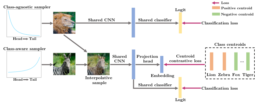
We propose interpolative contrastive centroid learning (ICCL), a framework to learn more discriminative representations for tail classes. The intuition behind our method is to use the head classes to facilitate representation learning of the tail classes. Inspired by Mixup [57], we create virtual training samples by interpolating two images from two samplers: a class-agnostic sampler which returns all images with equal probability, and a class-aware sampler which focuses more on tail-class images. The key idea of ICCL is shown in Figure 1. The representation of an interpolative sample should contain information that can be used to retrieve both the head-class centroid and the tail-class centroid. Specifically, we project images into a low-dimensional embedding space, and create class centroids as average embeddings. Given the embedding of the interpolative sample, we query the class centroids with a contrastive similarity matching, and train our model such that the embedding has higher similarities with the correct class centroids.
By injecting class-balanced knowledge in the form of centroids, the proposed interpolative centroid contrastive loss encourages the tail centroids to be positioned discriminatively relative to the head classes. However, the interpolative sample may conflate a head class and a tail class. Thus, we adopt the regular classification loss (top branch in Figure 2) to perform representation learning for head classes, so that the head classes themselves are well positioned. These loss components reinforce one another.
We evaluate the effectiveness of our approach on multiple standard benchmarks of different scale, including CIFAR-LT [1], ImageNet-LT [36] and iNaturalist 2018 [47]. We compare our methods with existing state-of-the-arts including Decouple [22], BBN [59], and De-confound-TDE [45].
We summarise our contribution as follows:
- •
We introduce interpolative centroid contrastive learning for discriminative long-tailed representation learning. ICCL reduces intra-class variance and increases inter-class variance by optimising the distance between sample embeddings and the class centroids.
- •
Different from previous findings that suggest class-agnostic training leads to high quality long-tailed representations, ICCL improves tail-class representations by addressing class imbalance with class-aware sample interpolation.
- •
ICCL achieves significantly high performance on multiple long-tailed recognition benchmarks. Notably, it achieves a substantial accuracy improvement of % on the large-scale iNaturalist 2018. We also perform ablation study to verify the effectiveness of each proposed component.
2 Related work
Re-sampling. Re-sampling aims to address the imbalance issue from the data level. Two main re-sampling approaches include oversampling and undersampling. Oversampling [2, 3, 15] increases the number of tail-class samples at the risk of overfitting the model, whereas undersampling might reduce the head classes diversity by decreasing their sample numbers [13, 35]. Class-balanced sampling assigns equal sampling probability for all classes, and then selects their respective images uniformly [42].
Re-weighting. Re-weighting methods modify the loss function algorithmically to improve the learning of tail classes [61, 23, 20, 30, 12, 44]. Cui et al. [8] introduced class-balanced loss based on the effective class samples, which improves upon the approaches that assign class weight inversely proportional to their sample number [40, 19, 38]. Another branch of work focuses on improving the decision boundary by enforcing margin between classes [1, 34, 33, 50, 11]. Menon et al. [39] proposed logit adjustment to softmax loss that considers the pairwise class relative margin from statistical perspective.
Feature Transfer. Another research direction for long-tailed recognition focuses on transferring the feature representation from head to tail classes [58, 32, 52, 9, 7]. OLTR [36] transfers features of head classes to tail classes using memory centroid features. Rather than just having a centroid for each category, Zhu et al. [62] extended OLTR by storing multiple features in both local and global memory bank to address the high intra-class variance issue.
Decoupled Strategy. Several studies have observed that applying re-sampling and re-weighting methods at the beginning of the training process will harm the learning of long-tailed representations [1, 59, 22]. BBN [59] introduces an extra re-balancing branch which focuses on tail classes. The conventional uniform branch and the re-balancing branch are trained simultaneously in a curriculum learning manner. Kang et al. [22] discovered that the long-tailed distribution has more negative impact on the classifier than the representation. They proposed a decoupled training approach, where it first performs representation learning without any re-sampling, and then rebalances the classifier in the second stage. Our method follows a similar two-stage training. However, we show that long-tailed representation learning can be further improved by our proposed interpolative centroid contrastive learning even before the classifier rebalancing stage.
It is worth noting that ensemble methods have also been proposed to improve long-tailed classification accuracy [54, 51, 59]. Wang et al. [51] reduced the computation complexity of ensemble by only assigning uncertain samples to extra experts dynamically.
Contrastive learning. Recently, contrastive learning approaches have demonstrated strong performance in self-supervised representation learning [4, 16, 5, 14, 53, 56]. Self-supervised contrastive learning projects images into low-dimensional embeddings, and performs similarity matching between images with different augmentations. Two augmented images from the same source image are encouraged to have higher similarity in contrast to others. Prototypical contrastive learning [29] introduces cluster-based prototypes and encourages embeddings to gather around their corresponding prototypes. MoPro [28] extends this idea to weakly-supervised learning and calculates prototypes based on exponential moving average.
Different from existing contrastive learning methods, our ICCL operates on an interpolative sample consisting information of both classes returned by the class-agnostic and class-aware sampler. Our contrastive loss seeks to learn a representation for the interpolative sample, such that it can be used to retrieve the centroids for both source classes. The centroid retrieval is performed via non-parametric contrastive similarity matching in the low-dimensional space, thus it is different from Mixup [57] which operates on the parametric classifier.
Mixup. As an effective data augmentation technique, Mixup [57] regularises the neural network by performing convex combination of training samples. Chou et al. [6] proposed larger mixing weight for tail classes to push the decision boundary towards the head classes. Several works have applied Mixup to improve contrastive learning representation in self-supervised setting [21, 25, 43, 60, 49, 27]. In contrast, our interpolative centroid contrastive loss is a new loss designed to improve supervised representation learning under long-tailed distribution.
3 Method
Formally speaking, for a long-tailed classification task, we are given a training dataset , where is an image and is its class label. The training dataset can be decomposed into , where comprises of head-class samples and consists of tail-class samples. Since , the model needs to learn strong discriminative representations for tail classes in a low-resource and imbalanced setting, such that it is not overwhelmed by the abundant head-class samples and is able to classify both head and tail classes correctly.
3.1 Overall framework
Our proposed long-tailed representation learning framework consists of a uniform and an interpolative branch as illustrated in Figure 2. The uniform branch follows the original long-tailed distribution to learn more generalisable representations from data-rich head-class samples, whereas the interpolative branch focuses more on modelling the tail-class to improve tail-class representation. Both branches share the same model parameters, which is different from BBN [59]. Next, we introduce the components of our framework:
- •
- •
A projection head which transforms the feature vector into a low-dimensional normalised embedding . Following SimCLR [4], the projection head is a MLP with one hidden layer of size and ReLU activations.
- •
A linear classifier with softmax activation which returns a class probability given a feature vector .
- •
Class centroids which resides in the low-dimensional embedding space. Similar to MoPro [28], we compute the centroid of each class as the exponential-moving-average (EMA) of the low-dimensional embeddings for samples from that class. Specifically, the centroid for class is updated during training by:
(1) where is the momentum coefficient.
- •
A class-agnostic and a class-aware sampler which create interpolative samples.
3.2 Interpolative sample generation
We utilise two different samplers for interpolative sample generation:
- •
A class-agnostic sampler which selects all samples with an equal probability regardless of the class, thus it returns more head-class samples. We denote a sample returned by the class-agnostic sampler as .
- •
A class-aware sampler which focuses more on tail classes. It first samples a class and then select the corresponding samples uniformly with repetition. Let denotes the number of samples in class , the probability of sampling class is inversely proportional to as follows:
(2) where is an adjustment parameter. When , the class-aware sampler is equivalent to the balanced sampler in [42]. When , it is the reverse sampler in [59]. We denote a sample returned by the class-aware sampler as .
An interpolative image is formed by linearly combining two images from the class-agnostic and class-aware sampler, respectively.
| (3) |
where is sampled from a uniform distribution. It is equivalent to the used in Mixup [57] with . Our contrastive learning trains the model such that the representation of the interpolative image is discriminative for both class and class .
3.3 Interpolative centroid contrastive loss
Here we introduce the proposed interpolative centroid contrastive loss which aims to improve long-tailed representation learning. Given the low-dimensional embedding for an interpolative sample , we use to query the class centroids with contrastive similarity matching. Specifically, the probability that the -th class centroid is retrieved is given as:
| (4) |
where is a scalar temperature parameter to scale the similarity. Equation 4 can be interpreted as a non-parametric classifier. Since the centroid is computed as the moving-average of , it does not suffer from the problem of weight imbalance as a parametric classifier does.
Since is a linear interpolation of and (see equation 3), our loss encourages the retrieval of the corresponding centroids of class and . Thus, the interpolative centroid contrastive loss is defined as:
| (5) |
The proposed centroid contrastive loss introduces valuable structural information into the embedding space. The numerator of reduces the intra-class variance by pulling embeddings with the same class closer to the class centroid. The denominator of increases the inter-class variance by pushing an embedding away from other classes’ centroids. Therefore, more discriminative representations can be learned.
| Dataset | Long-tailed CIFAR100 | Long-tailed CIFAR10 | ||||
| Imbalance ratio | 100 | 50 | 10 | 100 | 50 | 10 |
| CE∗ | 38.3 | 43.9 | 55.7 | 70.4 | 74.8 | 86.4 |
| Focal Loss∗ [30] | 38.4 | 44.3 | 55.8 | 70.4 | 76.7 | 86.7 |
| Mixup∗ [57] | 39.5 | 45.0 | 58.0 | 73.1 | 77.8 | 87.1 |
| Manifold Mixup∗ [48] | 38.3 | 43.1 | 56.6 | 73.0 | 78.0 | 87.0 |
| Manifold Mixup (two samplers)∗ [48] | 36.8 | 42.1 | 56.5 | 73.1 | 79.2 | 86.8 |
| CB-Focal∗ [8] | 39.6 | 45.2 | 58.0 | 74.6 | 79.3 | 87.1 |
| CE-DRW∗ [1] | 41.5 | 45.3 | 58.1 | 76.3 | 80.0 | 87.6 |
| CE-DRS∗ [1] | 41.6 | 45.5 | 58.1 | 75.6 | 79.8 | 87.4 |
| LDAM-DRW∗ [1] | 42.0 | 46.6 | 58.7 | 77.0 | 81.0 | 88.2 |
| cRT† [22] | 42.3 | 46.8 | 58.1 | 75.7 | 80.4 | 88.3 |
| LWS† [22] | 42.3 | 46.4 | 58.1 | 73.0 | 78.5 | 87.7 |
| BBN [59] | 42.6 | 47.0 | 59.1 | 79.8 | 82.2 | 88.3 |
| M2m [24] | 43.5 | - | 57.6 | 79.1 | - | 87.5 |
| De-confound-TDE [45] | 44.1 | 50.3 | 59.6 | 80.6 | 83.6 | 88.5 |
| ICCL (ours) | 46.6 | 51.6 | 62.1 | 82.1 | 84.7 | 89.7 |
3.4 Classification loss
Given the classifier’s output prediction probability for an image , we define the classification loss on the uniform branch as the standard cross entropy loss:
| (6) |
For an interpolative sample from the interpolative branch, the classification loss is
| (7) |
3.5 Overall loss
During training, we jointly minimise the sum of losses on both branches:
| (8) |
where and are the weights for the uniform branch and the interpolative branch, respectively.
3.6 Classifier rebalancing
Following the decoupled training approach [22], we rebalance our classifier after the representation learning stage. Specifically, we discard the projection head and fine-tune the linear classifier. The CNN encoder is either fixed or fine-tuned with a smaller learning rate. In order to rebalance the classifier towards tail classes, we employ our class-aware sampler. We denote the sampler’s adjustment parameter as . Due to more frequent sampling of tail-class samples by the class-aware sampler, the classifier’s logits distribution would shift towards the tail classes at the cost of lower accuracy on head classes. In order to maintain the head-class accuracy, we introduce a distillation loss [18, 46] using the classifier from the first stage as the teacher. The overall loss for classifier rebalancing consists of a cross-entropy classification loss and a KL-divergence distillation loss.
|
|
(9) |
where is the weight of the distillation loss, and are the class logits produced by the student classifier (2nd stage) and the teacher classifier (1st stage) , respectively. is the distillation temperature and is the softmax function.
For inference, we use a classification network consisting of the CNN encoder followed by the rebalanced classifier.
| Method | Overall | Many | Medium | Few |
| OLTR∗ [36] | 41.9 | 51.0 | 40.8 | 20.8 |
| Focal Loss∗ [30] | 43.7 | 64.3 | 37.1 | 8.2 |
| NCM [22] | 47.3 | 56.6 | 45.3 | 28.1 |
| -norm [22] | 49.4 | 59.1 | 46.9 | 30.7 |
| cRT [22] | 49.6 | 61.8 | 46.2 | 27.4 |
| LWS [22] | 49.9 | 60.2 | 47.2 | 30.3 |
| De-confound-TDE [45] | 51.8 | 62.7 | 48.8 | 31.6 |
| cRT† [22] | 52.4 | 64.3 | 49.1 | 30.7 |
| LWS† [22] | 52.5 | 63.0 | 49.6 | 32.8 |
| De-confound-TDE† [45] | 52.4 | 63.5 | 49.2 | 32.2 |
| ICCL (ours) | 54.0 | 60.7 | 52.9 | 39.0 |
4 Experiments
4.1 Dataset
We evaluate our method on three standard benchmark datasets for long-tail recognition as follows:
CIFAR-LT. CIFAR10-LT and CIFAR100-LT contain samples from the CIFAR10 and CIFAR100 [26] dataset, respectively. The class sampling frequency follows an exponential distribution. Following [59, 1], we construct LT datasets with different imbalance ratios of , , and . Imbalance ratio is defined as the ratio of maximum to the minimum class sampling frequency. The number of training images for CIFAR10-LT with an imbalance ratio of , and is k, k and k, respectively. Similarly, CIFAR100-LT has a training set size of k, k and k. Both test sets are balanced with the original size of k.
ImageNet-LT. The training set consists of classes with k images sampled from the ImageNet [10] dataset. The class sampling frequency follows a Pareto distribution with a shape parameter of [36]. The imbalance ratio is 256. Despite a smaller training size, it retains ImageNet [10] original test set size of k.
iNaturalist 2018. It is a real-world long-tailed dataset for fine-grained image classification of species [47]. We utilise the official training and test datasets composing of k training and k test images.
4.2 Evaluation
For all datasets, we evaluate our models on the test sets and report the overall top-1 accuracy across all classes. To further access the model’s accuracy on different classes, we group the classes into splits according to their number of images [36, 22]: many ( images), medium ( images) and few ( images).
4.3 Implementation details
For fair comparison, we follow the same training setup of previous works using SGD optimiser with a momentum of . For all experiments, we fix class centroid momentum coefficient , class-aware sampler adjustment parameter , , distillation weight and distillation temperature . Unless otherwise specified, for the hyperparameters, we set temperature , uniform branch weight , interpolative branch weight , and MLP projection head embedding size in the representation learning stage. In the classifier balancing stage, we freeze the CNN and fine-tune the classifier using the original learning rate with cosine scheduling [37] for epochs.
We also design a warm-up training curriculum. Specifically, In the first epochs, we train only the uniform branch using the cross-entropy loss and a (non-interpolative) centroid contrastive loss . After epochs, we activate the interpolative branch and optimise in Equation 8. The warm-up provides good initialisation for the representations and the centroids. is scheduled to be approximately halfway through the total number of epochs.
CIFAR-LT. We use a ResNet-32 [17] as the CNN encoder and follow the training strategies in [59]. We train the model for epochs with a batch size of . The projected embedding size is . We use standard data augmentation which consists of random horizontal flip and cropping with a padding size of . The learning rate warms up to within the first epochs and decays at epoch and with a step size of . We use a weight decay of . We set and as and epochs for CIFAR100-LT and CIFAR10-LT, respectively. is set as 0 after warm-up. In the classifier balancing stage, we fine-tune the CNN encoder using cosine scheduling with an initial learning rate of .
ImageNet-LT. We train a ResNeXt-50 [55] model for epochs using a batch size of , a weight decay of , and a base learning rate of with cosine scheduling. Similar to [22], we augment the data using random horizontal flip, cropping and colour jittering. We set .
iNaturalist 2018. Following [22], we train a ResNet-50 model for epochs and epochs using learning rate with cosine decay, batch size and weight decay. The data augmentation comprises of only horizontal flip and cropping. is set as and epochs for training epochs of and , respectively.
4.4 Results
| Method | 90 Epochs | 200 Epochs | ||||||
| Overall | Many | Medium | Few | Overall | Many | Medium | Few | |
| CB-Focal [8] | 61.1 | - | - | - | - | - | - | - |
| CE-DRS∗ [1] | 63.6 | - | - | - | - | - | - | - |
| CE-DRW∗ [1] | 63.7 | - | - | - | - | - | - | - |
| LDAM-DRW [1] | 68.0 | - | - | - | - | - | - | - |
| LDAM-DRW∗ [1] | 64.6 | - | - | - | 66.1 | - | - | - |
| NCM [22] | 58.2 | 55.5 | 57.9 | 59.3 | 63.1 | 61.0 | 63.5 | 63.3 |
| cRT [22] | 65.2 | 69.0 | 66.0 | 63.2 | 68.2 | 73.2 | 68.8 | 66.1 |
| -norm [22] | 65.6 | 65.6 | 65.3 | 65.9 | 69.3 | 71.1 | 68.9 | 69.3 |
| LWS [22] | 65.9 | 65.0 | 66.3 | 65.5 | 69.5 | 71.0 | 69.8 | 68.8 |
| BBN [59] | 66.4 | 49.4 | 70.8 | 65.3 | 69.7 | 61.7 | 73.6 | 66.9 |
| ICCL (ours) | 70.5 | 67.6 | 70.2 | 71.6 | 72.5 | 72.1 | 72.3 | 72.9 |
Next we present the results, where the proposed ICCL achieves significant improved performance on all benchmarks.
CIFAR-LT. Table 1 demonstrates that ICCL surpasses existing methods across different imbalance ratios for both CIFAR100-LT and CIFAR10-LT. Notably, after the representation learning stage, our approach generally achieves competitive performance compared to existing methods apart from De-confound-TDE [45]. By balancing the classifier, the performance of ICCL further improves and outperforms De-confound-TDE by % on the more challenging CIFAR100-LT with imbalance ratio of .
ImageNet-LT. Table 2 presents the ImageNet-LT results, where ICCL outperforms the existing methods. For ImageNet-LT, we also propose an improved set of hyperparameters which increases the accuracy for existing methods. Specifically, different from the original hyperparameters used in [22], we use a smaller batch size of and a learning rate of . Furthermore, we find it is better to use original learning rate for classifier balancing. For fair comparison, we re-implement Decouple methods [22] and De-confound-TDE [45] using our settings and obtain better accuracy than those reported in the original papers. However, ICCL still achieves the best overall accuracy of % with noticeable accuracy gains on medium and few classes.
iNaturalist 2018. On the real-world large-scale iNaturalist 2018 dataset, ICCL achieves substantial improvements compared with existing methods as shown in Table 3. For and epochs, our method surpasses BBN [59] by % and % respectively. We obtain the split accuracy of BBN based on the checkpoint released by the authors. We observe that BBN suffers from a large discrepancy of % between the many and medium class accuracy for epochs, whereas our method has more consistent accuracy across all splits. Additionally, ICCL obtains a best overall accuracy of % at epochs which is better than BBN (%) at epochs.
4.5 Ablation study
Here we perform extensive ablation study to examine the effect of each component and hyperparameters of ICCL, and provide analysis on what makes ICCL successful.
| Warm-up | Overall | Head | Tail | |||
| ✓ | 51.3 | 60.6 | 45.5 | |||
| ✓ | 51.6 | 58.3 | 47.4 | |||
| ✓ | ✓ | 51.7 | 57.9 | 47.9 | ||
| ✓ | ✓ | ✓ | 52.4 | 59.9 | 47.7 | |
| ✓ | ✓ | ✓ | 53.4 | 61.1 | 48.6 | |
| ✓ | ✓ | ✓ | 53.6 | 61.2 | 48.8 | |
| ✓ | ✓ | ✓ | ✓ | 54.0 | 60.7 | 49.8 |
| CIFAR100-LT | |
| (0.2, 1.0) | 43.6 |
| (0.2, 0.2) | 43.8 |
| (0.6,0.6) | 45.4 |
| (1.0,1.0) | 46.6 |
| (2.0, 2.0) | 46.8 |
Loss components. For representation learning, ICCL introduces the interpolative centroid contrastive loss and the interpolative cross-entropy loss as shown in Equation 8. In Table 4, we evaluate the contribution of each loss components using ImageNet-LT dataset. We consider many split as the head classes ( images per class), medium and few splits as the tail classes ( images per class). We employ the same classifier balancing technique as described in Section 3.4. We observe that both and improve the overall accuracy individually and collectively. By comparing with only which is equivalent to Mixup [57], we demonstrate that our loss formulation achieves superior performance. Additionally, having a warm-up before incorporating interpolative losses provides an extra accuracy boost, especially for the tail classes. This aligns with the observation in [1] which suggests that adopting a deferred schedule before re-sampling is better for representation learning.
| Sampler | CIFAR100-LT | CIFAR10-LT | ImageNet-LT | iNaturalist |
| Uniform | 44.7 | 79.9 | 52.8 | 69.4 |
| 46.6 | 82.1 | 54.0 | 70.5 | |
| 46.2 | 81.6 | 54.1 | 70.2 | |
| 46.2 | 81.1 | 53.1 | 70.1 |

Interpolation weight . In Equation 3, We sample the interpolation weight from a uniform distribution, which is equivalent to . We vary the beta distribution and study its effect on CIFAR100-LT with an imbalance ratio of . The resulting accuracy and the corresponding beta distribution are shown in Table 5. Sampling from is more likely to return a small , thus the interpolative samples contain more information about images from the class-aware sampler. As we fix and increase them from to , the accuracy increases. Good performance can be achieved with and , where the sampled is less likely to be an extreme value.
Class-aware sampler adjustment parameter . We further investigate the influence of on representation learning. When and , the class-aware sampler is equivalent to class-balanced sampler [42] and reverse sampler [59] respectively. We include a class-agnostic uniform sampler as the baseline. Table 6 shows that the interpolative branch sampler should neither focus excessively on the tail classes () nor on the head classes (uniform). When using either of these two samplers, the resulting interpolative image might be less informative due to excessive repetition of tail-class samples or redundant head-class samples.
| Method | Rebalancing | Overall | Many | Medium | Few |
| CE [22] | - | 46.7 | 68.1 | 40.2 | 9.0 |
| ICCL (ours) | - | 50.5 | 68.5 | 44.4 | 20.8 |
| CE [22] | ✓ | 52.4 | 64.3 | 49.1 | 30.7 |
| ICCL (ours) | ✓ | 54.0 | 60.7 | 52.9 | 39.0 |

Rebalancing classifier. In Table 7, we show the effect of classifier rebalancing, which improves both ICCL and the baseline CE method [22]. By learning better tail-class representation, ICCL achieves higher overall accuracy compared to [22] both before and after classifier rebalancing.
Classifier balancing parameters. In the classifier balancing stage, we fix the sampler adjustment parameter , and the distillation weight . We study their effects in Table 8. For our ICCL approach, using a reverse sampler () is better than a balanced sampler (). Furthermore, the distillation loss tends to benefit more complex ImageNet-LT and iNaturalist than CIFAR-LT datasets. For the baseline cRT [22], applying the reverse sampler and distillation does not give accuracy improvement compared to the default setting (52.4).
| CIFAR100-LT | CIFAR10-LT | iNaturalist | ImageNet-LT | |||
| ICCL | ICCL | ICCL | ICCL | cRT [22] | ||
| 0 | 0 | 45.3 | 77.5 | 69.5 | 53.7 | 52.4 |
| 0 | 0.5 | 45.0 | 77.6 | 69.5 | 53.2 | 52.2 |
| 1 | 0 | 47.1 | 82.3 | 70.2 | 53.6 | 49.6 |
| 1 | 0.5 | 46.6 | 82.1 | 70.5 | 54.0 | 51.3 |
Weight norm visualisation. The norms of the weights for the linear classification layer suggest how balanced the classifier is. Having a high weight norm for a particular class indicates that the classifier is more likely to generate a high logit score for that class. Figure 3 depicts the weight norm of ICCL and cRT [22] after the representation learning and classifier balancing stage. In both stages, our ICCL classifier has a more balanced weight norm compared with cRT. Furthermore, we also plot the norm of our class centroids , which shows that the centroids are intrinsically balanced across different classes.
Distillation temperature . In Figure 4, we study how affects the accuracy of ICCL on ImageNet-LT. We find that the overall accuracy is not sensitive to changes in . As increases, the teacher’s logit distribution becomes more flattened. Therefore, the accuracy for medium and few class improves, whereas the accuracy for many class decreases.
5 Conclusion
In this work, we propose an interpolative centroid contrastive learning technique for long-tailed representation learning. By utilising class centroids and interpolative losses, we strengthen the discriminative power of the learned representations, leading to improved classification accuracy. We demonstrate the effectiveness of our approach with significant improvement on multiple long-tailed classification benchmarks.
6 Acknowledgments
Anthony Meng Huat Tiong is supported by Salesforce and the Singapore Economic Development Board under the Industrial Postgraduate Programme. Boyang Li is supported by the Nanyang Associate Professorship and the National Research Foundation Fellowship (NRF-NRFF13-2021-0006), Singapore. Any opinions, findings, conclusions, or recommendations expressed in this material are those of the authors and do not reflect the views of the funding agencies.
References
- [1] Kaidi Cao, Colin Wei, Adrien Gaidon, Nikos Arechiga, and Tengyu Ma. Learning imbalanced datasets with label-distribution-aware margin loss. In NeurIPS, pages 1567–1578, 2019.
- [2] Nitesh V Chawla, Kevin W Bowyer, Lawrence O Hall, and W Philip Kegelmeyer. Smote: synthetic minority over-sampling technique. Journal of artificial intelligence research, 16:321–357, 2002.
- [3] Nitesh V Chawla, Aleksandar Lazarevic, Lawrence O Hall, and Kevin W Bowyer. Smoteboost: Improving prediction of the minority class in boosting. In European conference on principles of data mining and knowledge discovery, pages 107–119. Springer, 2003.
- [4] Ting Chen, Simon Kornblith, Mohammad Norouzi, and Geoffrey Hinton. A simple framework for contrastive learning of visual representations. In ICML, 2020.
- [5] Xinlei Chen, Haoqi Fan, Ross Girshick, and Kaiming He. Improved baselines with momentum contrastive learning. arXiv preprint arXiv:2003.04297, 2020.
- [6] Hsin-Ping Chou, Shih-Chieh Chang, Jia-Yu Pan, Wei Wei, and Da-Cheng Juan. Remix: Rebalanced mixup. In ECCV, pages 95–110. Springer, 2020.
- [7] Peng Chu, Xiao Bian, Shaopeng Liu, and Haibin Ling. Feature space augmentation for long-tailed data. In ECCV, 2020.
- [8] Yin Cui, Menglin Jia, Tsung-Yi Lin, Yang Song, and Serge Belongie. Class-balanced loss based on effective number of samples. In CVPR, pages 9268–9277, 2019.
- [9] Yin Cui, Yang Song, Chen Sun, Andrew Howard, and Serge Belongie. Large scale fine-grained categorization and domain-specific transfer learning. In CVPR, pages 4109–4118, 2018.
- [10] Jia Deng, Wei Dong, Richard Socher, Li-Jia Li, Kai Li, and Fei-Fei Li. Imagenet: A large-scale hierarchical image database. In CVPR, pages 248–255, 2009.
- [11] Jiankang Deng, Jia Guo, Niannan Xue, and Stefanos Zafeiriou. Arcface: Additive angular margin loss for deep face recognition. In CVPR, pages 4690–4699, 2019.
- [12] Qi Dong, Shaogang Gong, and Xiatian Zhu. Class rectification hard mining for imbalanced deep learning. In ICCV, pages 1851–1860, 2017.
- [13] Chris Drummond, Robert C Holte, et al. C4. 5, class imbalance, and cost sensitivity: why under-sampling beats over-sampling. In Workshop on learning from imbalanced datasets II, volume 11, pages 1–8. Citeseer, 2003.
- [14] Jean-Bastien Grill, Florian Strub, Florent Altché, Corentin Tallec, Pierre H. Richemond, Elena Buchatskaya, Carl Doersch, Bernardo Avila Pires, Zhaohan Daniel Guo, Mohammad Gheshlaghi Azar, Bilal Piot, Koray Kavukcuoglu, Rémi Munos, and Michal Valko. Bootstrap your own latent: A new approach to self-supervised learning. arXiv preprint arXiv:2006.07733, 2020.
- [15] Hui Han, Wen-Yuan Wang, and Bing-Huan Mao. Borderline-smote: a new over-sampling method in imbalanced data sets learning. In International conference on intelligent computing, pages 878–887. Springer, 2005.
- [16] Kaiming He, Haoqi Fan, Yuxin Wu, Saining Xie, and Ross Girshick. Momentum contrast for unsupervised visual representation learning. In Proceedings of the IEEE/CVF Conference on Computer Vision and Pattern Recognition, pages 9729–9738, 2020.
- [17] Kaiming He, Xiangyu Zhang, Shaoqing Ren, and Jian Sun. Deep residual learning for image recognition. In CVPR, pages 770–778, 2016.
- [18] Geoffrey Hinton, Oriol Vinyals, and Jeff Dean. Distilling the knowledge in a neural network. arXiv preprint arXiv:1503.02531, 2015.
- [19] Chen Huang, Yining Li, Chen Change Loy, and Xiaoou Tang. Learning deep representation for imbalanced classification. In CVPR, pages 5375–5384, 2016.
- [20] Muhammad Abdullah Jamal, Matthew Brown, Ming-Hsuan Yang, Liqiang Wang, and Boqing Gong. Rethinking class-balanced methods for long-tailed visual recognition from a domain adaptation perspective. In CVPR, pages 7610–7619, 2020.
- [21] Yannis Kalantidis, Mert Bulent Sariyildiz, Noe Pion, Philippe Weinzaepfel, and Diane Larlus. Hard negative mixing for contrastive learning. In NeurIPS, 2020.
- [22] Bingyi Kang, Saining Xie, Marcus Rohrbach, Zhicheng Yan, Albert Gordo, Jiashi Feng, and Yannis Kalantidis. Decoupling representation and classifier for long-tailed recognition. In ICLR, 2020.
- [23] Salman H Khan, Munawar Hayat, Mohammed Bennamoun, Ferdous A Sohel, and Roberto Togneri. Cost-sensitive learning of deep feature representations from imbalanced data. IEEE transactions on neural networks and learning systems, 29(8):3573–3587, 2017.
- [24] Jaehyung Kim, Jongheon Jeong, and Jinwoo Shin. M2m: Imbalanced classification via major-to-minor translation. In Proceedings of the IEEE/CVF Conference on Computer Vision and Pattern Recognition, pages 13896–13905, 2020.
- [25] Sungnyun Kim, Gihun Lee, Sangmin Bae, and Se-Young Yun. Mixco: Mix-up contrastive learning for visual representation. In NeurIPS Workshop, 2020.
- [26] Alex Krizhevsky and Geoffrey Hinton. Learning multiple layers of features from tiny images. Technical report, 2009.
- [27] Kibok Lee, Yian Zhu, Kihyuk Sohn, Chun-Liang Li, Jinwoo Shin, and Honglak Lee. i-mix: A domain-agnostic strategy for contrastive representation learning. In ICLR, 2021.
- [28] Junnan Li, Caiming Xiong, and Steven CH Hoi. Mopro: Webly supervised learning with momentum prototypes. arXiv preprint arXiv:2009.07995, 2020.
- [29] Junnan Li, Pan Zhou, Caiming Xiong, Richard Socher, and Steven C.H. Hoi. Prototypical contrastive learning of unsupervised representations. arXiv preprint arXiv:2005.04966, 2020.
- [30] Tsung-Yi Lin, Priya Goyal, Ross Girshick, Kaiming He, and Piotr Dollár. Focal loss for dense object detection. In ICCV, pages 2980–2988, 2017.
- [31] Tsung-Yi Lin, Michael Maire, Serge Belongie, James Hays, Pietro Perona, Deva Ramanan, Piotr Dollár, and C Lawrence Zitnick. Microsoft coco: Common objects in context. In ECCV, pages 740–755. Springer, 2014.
- [32] Jialun Liu, Yifan Sun, Chuchu Han, Zhaopeng Dou, and Wenhui Li. Deep representation learning on long-tailed data: A learnable embedding augmentation perspective. In CVPR, pages 2970–2979, 2020.
- [33] Weiyang Liu, Yandong Wen, Zhiding Yu, Ming Li, Bhiksha Raj, and Le Song. Sphereface: Deep hypersphere embedding for face recognition. In CVPR, pages 212–220, 2017.
- [34] Weiyang Liu, Yandong Wen, Zhiding Yu, and Meng Yang. Large-margin softmax loss for convolutional neural networks. In ICML, volume 2, page 7, 2016.
- [35] Xu-Ying Liu, Jianxin Wu, and Zhi-Hua Zhou. Exploratory undersampling for class-imbalance learning. IEEE Transactions on Systems, Man, and Cybernetics, Part B (Cybernetics), 39(2):539–550, 2008.
- [36] Ziwei Liu, Zhongqi Miao, Xiaohang Zhan, Jiayun Wang, Boqing Gong, and Stella X. Yu. Large-scale long-tailed recognition in an open world. In CVPR, pages 2537–2546, 2019.
- [37] Ilya Loshchilov and Frank Hutter. Sgdr: Stochastic gradient descent with warm restarts. arXiv preprint arXiv:1608.03983, 2016.
- [38] Dhruv Mahajan, Ross Girshick, Vignesh Ramanathan, Kaiming He, Manohar Paluri, Yixuan Li, Ashwin Bharambe, and Laurens van der Maaten. Exploring the limits of weakly supervised pretraining. In ECCV, pages 181–196, 2018.
- [39] Aditya Krishna Menon, Sadeep Jayasumana, Ankit Singh Rawat, Himanshu Jain, Andreas Veit, and Sanjiv Kumar. Long-tail learning via logit adjustment. ICLR, 2021.
- [40] Tomas Mikolov, Ilya Sutskever, Kai Chen, Greg S Corrado, and Jeff Dean. Distributed representations of words and phrases and their compositionality. In NeurIPS, pages 3111–3119, 2013.
- [41] David MW Powers. Applications and explanations of zipf’s law. In New methods in language processing and computational natural language learning, 1998.
- [42] Li Shen, Zhouchen Lin, and Qingming Huang. Relay backpropagation for effective learning of deep convolutional neural networks. In ECCV, pages 467–482. Springer, 2016.
- [43] Zhiqiang Shen, Zechun Liu, Zhuang Liu, Marios Savvides, Trevor Darrell, and Eric Xing. Un-mix: Rethinking image mixtures for unsupervised visual representation learning. arXiv preprint arXiv:2003.05438, 2020.
- [44] Jun Shu, Qi Xie, Lixuan Yi, Qian Zhao, Sanping Zhou, Zongben Xu, and Deyu Meng. Meta-weight-net: Learning an explicit mapping for sample weighting. In NeurIPS, pages 1919–1930, 2019.
- [45] Kaihua Tang, Jianqiang Huang, and Hanwang Zhang. Long-tailed classification by keeping the good and removing the bad momentum causal effect. In NeurIPS, 2020.
- [46] Yonglong Tian, Dilip Krishnan, and Phillip Isola. Contrastive representation distillation. In ICLR, 2020.
- [47] Grant Van Horn, Oisin Mac Aodha, Yang Song, Yin Cui, Chen Sun, Alex Shepard, Hartwig Adam, Pietro Perona, and Serge Belongie. The inaturalist species classification and detection dataset. In CVPR, pages 8769–8778, 2018.
- [48] Vikas Verma, Alex Lamb, Christopher Beckham, Amir Najafi, Ioannis Mitliagkas, David Lopez-Paz, and Yoshua Bengio. Manifold mixup: Better representations by interpolating hidden states. In ICML, pages 6438–6447. PMLR, 2019.
- [49] Vikas Verma, Minh-Thang Luong, Kenji Kawaguchi, Hieu Pham, and Quoc V Le. Towards domain-agnostic contrastive learning. In ICML, 2021.
- [50] Hao Wang, Yitong Wang, Zheng Zhou, Xing Ji, Dihong Gong, Jingchao Zhou, Zhifeng Li, and Wei Liu. Cosface: Large margin cosine loss for deep face recognition. In CVPR, pages 5265–5274, 2018.
- [51] Xudong Wang, Long Lian, Zhongqi Miao, Ziwei Liu, and Stella X Yu. Long-tailed recognition by routing diverse distribution-aware experts. ICLR, 2021.
- [52] Yu-Xiong Wang, Deva Ramanan, and Martial Hebert. Learning to model the tail. In NeurIPS, pages 7029–7039, 2017.
- [53] Zhirong Wu, Yuanjun Xiong, Stella X. Yu, and Dahua Lin. Unsupervised feature learning via non-parametric instance discrimination. In CVPR, pages 3733–3742, 2018.
- [54] Liuyu Xiang and Guiguang Ding. Learning from multiple experts: Self-paced knowledge distillation for long-tailed classification. In ECCV, 2020.
- [55] Saining Xie, Ross Girshick, Piotr Dollár, Zhuowen Tu, and Kaiming He. Aggregated residual transformations for deep neural networks. In Proceedings of the IEEE conference on computer vision and pattern recognition, pages 1492–1500, 2017.
- [56] Yuzhe Yang and Zhi Xu. Rethinking the value of labels for improving class-imbalanced learning. In NeurIPS, 2020.
- [57] Hongyi Zhang, Moustapha Cisse, Yann N Dauphin, and David Lopez-Paz. mixup: Beyond empirical risk minimization. In ICLR, 2018.
- [58] Yaoyao Zhong, Weihong Deng, Mei Wang, Jiani Hu, Jianteng Peng, Xunqiang Tao, and Yaohai Huang. Unequal-training for deep face recognition with long-tailed noisy data. In CVPR, pages 7812–7821, 2019.
- [59] Boyan Zhou, Quan Cui, Xiu-Shen Wei, and Zhao-Min Chen. BBN: Bilateral-branch network with cumulative learning for long-tailed visual recognition. pages 1–8, 2020.
- [60] Hong-Yu Zhou, Shuang Yu, Cheng Bian, Yifan Hu, Kai Ma, and Yefeng Zheng. Comparing to learn: Surpassing imagenet pretraining on radiographs by comparing image representations. In MICCAI. Springer, 2020.
- [61] Zhi-Hua Zhou and Xu-Ying Liu. Training cost-sensitive neural networks with methods addressing the class imbalance problem. IEEE Transactions on knowledge and data engineering, 18(1):63–77, 2005.
- [62] Linchao Zhu and Yi Yang. Inflated episodic memory with region self-attention for long-tailed visual recognition. In CVPR, pages 4344–4353, 2020.