UniFed: A Unified Framework for Federated Learning on Non-IID Image Features

Recent FL studies have been increasingly investigating the issue of non-iid data distributions across different clients, from multiple aspects, such as federated training, client model personalization, and federated generalization. Most existing works aim to improve federated training, such as regularizing local model training [33, 3, 34], facilitating model optimization [13, 35, 36], enhancing aggregation algorithm [37, 38], improving feature normalization [27, 39, 40], etc. For example, as an early work, FedProx [33] extends the conventional FedAvg [8] by adding a proximal term to help regularize the client training. SCAFFOLD [13] suggests a new optimization algorithm to reduce variance for client drift in its local updates. Later on, FedNova [37] proposes to use normalized stochastic gradients to perform global model aggregation rather than the cumulative raw local gradient changes; MOON [34] proposes to use contrastive learning on latent feature representations to enhance the agreements between local and global models. Very recently, FedDC [36] improved the SCAFFOLD [13] by dynamically updating the objective function of each client, which contains a constraint penalty term and a gradient correction term.

Instead of learning a common global model, another promising direction for tackling non-iid data issue is learning personalized models. Personalized FL targets adapting the common consensus model to fit each client’s individual data distribution. For example, PerFedAvg [41] introduces meta-learning in FL to obtain a personalized variant of FedAvg; Ditto [42] utilizes regularization terms and multi-task learning objectives to train personalized models; FedBABU [43] proposes to share encoders across clients but preserve classifiers locally to perform the personalization.

Besides federated training on non-iid data, another important direction is federated generalization, which aims to improve the generalizability of federated models on unseen clients outside the federation. FedDG [14] first proposes this setting on medical images, and it presents a method to share client distribution information in a privacy-protecting way. FedADG [15] extends federated generalization to natural images and proposes to use federated adversarial learning to measure and align distributions among different clients. Recently, Yuan et al. [44] studied the generalization gap by considering two levels, i.e., out-of-sample gap and participation gap, and proposed a semantic synthesis strategy that enables realistic simulation without naturally-partitioned data; Caldarola et al. [45] improve generalization in federated learning by employing sharpness-aware minimization and averaging stochastic weights.

Many efforts have been made to improve the FL on non-iid data, but all these existing works focus on boosting performance for clients either inside or outside the federation. There is still no unified solution to consider all these comprehensive scenarios jointly.

Not only in the context of FL, the data heterogeneity issue has also been studied in many scenarios, such as multi-site learning, domain adaptation, and domain generalization. These works further motivate the emergency need for one unified framework to tackle the heterogeneity issue in internal and external data simultaneously. For example, in multi-site learning [18, 46] works, experiments show that the model suffers a significant performance drop on external validation data. In domain adaptation and generalization which focus on improving performance for target (external) domain, a key idea is forcing a model to be domain agnostic. This idea essentially averages the domain conflict, thus the performance drops on each source (internal) domain [47]. Galstyan et al. [48] also propose to measure metrics on training data when designing domain generalization algorithms. These works only focus on internal training or external testing, but all emphasize the importance of designing well-performing algorithms on both internal and external data. Therefore, a unified framework is highly demanded.

Batch Normalization [24] is an indispensable component in many deep neural networks and has shown its success in neural network training. Relevant literature has uncovered several benefits given by batch normalization. Santurkar et al. [25] show that BN makes the optimization landscape significantly smoother during training process, the smoothness induces a more predictive and stable behavior of the gradients. Luo et al. [49] decompose BN into population normalization and gamma decay, and consider it an implicit regularizer to improve the robustness of optimization. Yang et al. [50] provide a characterization of signal propagation and gradient backpropagation in wide BN networks at initialization. Morcos et al. [51] suggest that BN implicitly discourages single direction reliance, thus improving the model generalizability. Li et al. [52] take advantage of BN for tackling the domain adaptation problem. However, besides our early work [27], very limited study [40] considers the effects of BN in FL, and only empirical results are demonstrated. It is unclear what role BN plays in the scope of FL, especially for non-iid data. Comprehensive theoretical and empirical studies still remain unexplored to date.

We start with the formulation for FL on non-iid data with feature shifts. We assume $N\in\mathbb{N}$ clients jointly train for $T\in\mathbb{N}$ rounds. Denote the input space $\X\subset\mathbb{R}^{d}$ and the label space $\Y\subset\mathbb{R}$, where $d$ is the input dimension. Let $\mathbf{x}\in\X$ and $y\in\Y$ be the input and output random variables following an underlying joint distribution $\D$ with density $p(\mathbf{x},y)$.

For each client $i\in[N]$ ($[N]=\{1,\dots,N\}$), it has access to a training set of samples drawn from $\D_{i}$. By rewriting $p_{i}(\mathbf{x},y)$ as $p_{i}(y|\mathbf{x})p_{i}(\mathbf{x})$ and $p_{i}(\mathbf{x}|y)p_{i}(y)$, we define feature shift as: 1) covariate shift: the $p_{i}(\mathbf{x})$ varies across clients, while $p_{i}(y|\mathbf{x})$ is the same for all clients; and 2) concept shift: the $p_{i}(\mathbf{x}|y)$ varies across clients and $p(y)$ is the same. Let $f:\mathbb{R}^{d}\rightarrow\mathbb{R}$ be a model, each client aims to train its local model $f_{i}$ by minimizing the following risk:

where $\mathbb{E}$ denotes the expectation and $\ell$ is a proper loss function, e.g., the mean squared error loss function for the regression or the cross-entropy loss for the classification task. The overall goal of FL is that $N$ clients collaboratively train a global model $f$ by minimizing the aggregated risk:

The overall goal of FL is to train a global model $f$ that generalizes well with respect to $p(\mathbf{x},y)$. In practice, empirical risk minimization is commonly used as an approximation of $J_{i}(f_{i})$ based on the client’s local data. Since aggregated risk minimization is performed without sharing clients’ local data, the non-iid features issue brings challenges from two aspects. First, the local risk minimization differs due to non-iid features, this diverges the aggregated risk minimization and harms the convergence rate. Second, the global model trained on heterogeneous features via the aggregated risk is not guaranteed to be an accurate estimation for each specific client, causing high generalization errors on testing clients. The error would largely increase when testing on external clients. It is a critical issue, because, in real-world settings, many clients may never participate in training [11, 44].

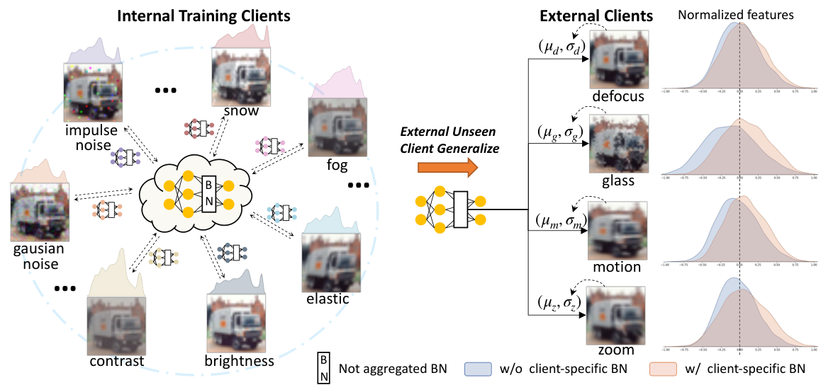
In this regard, we propose an efficient and effective framework UniFed to address the non-iid features issue. Our approach solves the joint risk minimization problem in Eq.(2) by tacking feature shifts via BN statistics calculated from each local client. Fig. 1 shows the overview of our framework, images over clients have non-iid features, and each client uses client-specific BN to tackle the non-iid features. Our framework considers two stages: federated training and federated testing. We present the full algorithm in Algorithm 1. For federated training, each client preserves its own BN layers by excluding its parameters from the aggregation. For federated testing, if the client presented during training, we directly use the client model $w_{i}^{T}$, which only differs from the global model $w^{T}$ regarding client-specific BN parameters. If the client does not participate in training (a.k.a. external client), the client-specific BN strategy proposes re-estimating test data statistics for BN layers. Specifically, given an external client with batches of data to be tested sequentially (each batch has $n_{t}$ samples). The mean term $\mu$ and variance term $\sigma$ are calculated as:

Since the batch-level sampling may not accurately estimate the population-level mean and variance for a client, to stabilize the fluctuation, we further propose to use a momentum term $\tau$ to integrate relations among different batches:

Our proposed client-specific BN results in significant empirical improvements in non-iid settings. We provide an explanation for these improvements by presenting theoretical analysis to show that our framework improves the convergence rate and yields a lower generalization error bound.

Here we study the property of faster convergence by comparing our framework with and without client-specific BN. Our main idea is to study the training dynamics of networks through the neural tangent kernel (NTK) [28]. For simplicity, we assume all clients to have $M\in\mathbb{N}$ training examples for a regression task, i.e., each client $i\in[N]$ has training examples $\{(\mathbf{x}^{i}_{j},y^{i}_{j})\in\mathbb{R}^{d}\times\mathbb{R}:j\in[M]\}$. Furthermore, we assume $f$ a two-layer ReLU neural network parameterized by $(\mathbf{W},\mathbf{c})\in\mathbb{R}^{m\times d}\times\mathbb{R}^{m}$ as:

where $\phi(s)=\max\{s,0\}$ is the ReLU activation function. $\mathbf{w}_{k}\in\mathbb{R}^{d}$ denotes the parameters of the first layer, where $k\in[m]$ and $m$ is the width of the hidden layer. $\mathbf{c}$ is the top layer parameters of the network. Let $\parallel\mathbf{w}\parallel_{\mathbf{S}}\triangleq\sqrt{\mathbf{w}^{\top}\mathbf{S}\mathbf{w}}$ denote the induced vector norm for a positive definite matrix $\mathbf{S}$. To investigate the gradient descent training with BN, we make the following assumption.

With Assumption III.1, we incorporate the analysis on BN by drawing the following analogy, where batch training with BN amounts to:

where $\gamma$ is the scaling parameter of BN.

Now we define our framework with client-specific BN parameters as $f^{*}:\mathbb{R}^{d}\rightarrow\mathbb{R}$ by re-parameterizing the Eq.(5) with $(\mathbf{V},\mathbf{\gamma},\mathbf{c})\in\mathbb{R}^{m\times d}\times\mathbb{R}^{m\times N}\times\mathbb{R}^{m}$, i.e.,

where the normalization of the first layer for client $i$ is $\frac{\mathbf{v}_{k}^{\top}\mathbf{x}^{i}}{\parallel\mathbf{v}_{k}\parallel_{\mathbf{S}_{i}}}$. Here, we omit learning the shift parameter of BN ¹¹ 1 We omit centering neurons as well as learning the shift parameter of BN for the neural network analysis because of the assumption that $\mathbf{x}$ is zero-mean and the two-layer network setting [53, 54].. If using aggregated BN, the framework instead trains a function $f:\mathbb{R}^{d}\rightarrow\mathbb{R}$ which is a special case of Eq. (7) with $\gamma_{k,i}=\gamma_{k}$ for $\forall i\in[N]$. We take a random initialization of the parameters [54] in our analysis:

where $\alpha^{2}$ controls the magnitude of $\mathbf{v}_{k}$ at initialization. The initialization of the BN parameters $\gamma_{k}$ and $\gamma_{k,i}$ are independent of $\alpha$. The parameters of the network $f^{*}(\mathbf{x};\mathbf{V},\mathbf{\gamma},\mathbf{c})$ are obtained by minimizing the empirical risk derived from Eq.(1). The loss function $\ell$ is chosen to be the squared loss, i.e., $\ell=(f^{*}(\mathbf{x}_{i})-y_{i})^{2}$.

Then we study the trajectory of networks with aggregated BN ($f$) and with client-specific BN (ours) ($f^{*}$) through the NTK introduced by [28]. Recent machine learning theory studies [55, 56, 57, 58, 59] have shown that for finite-width over-parameterized networks, the convergence rate is controlled by the least eigenvalue of the induced kernel in the training evolution.

We can decompose the NTK into a magnitude component $\mathbf{G}(t)$ and direction component $\mathbf{V}(t)/\alpha^{2}$ following [59]:

The specific forms of $\mathbf{V}(t)$ and $\mathbf{G}(t)$ are given in Appendix A-A. Let $\lambda_{min}(A)$ denote the minimal eigenvalue of matrix $A$. The matrices $\mathbf{V}(t)$ and $\mathbf{G}(t)$ are positive semi-definite, since they can be viewed as covariance matrices. This gives $\lambda_{\min}(\mathbf{\Lambda}(t))\geq\max\left\{\lambda_{\min}(\mathbf{V}(t))/\alpha^{2},\lambda_{\min}(\mathbf{G}(t))\right\}$. According to NTK, the convergence rate is controlled by $\lambda_{min}(\mathbf{\Lambda}(t))$. Then, for $\alpha>1$, convergence is dominated by $\mathbf{G}(t)$. Let $\mathbf{\Lambda}(t)$ denote the evolution dynamics of network with aggregated BN, and $\mathbf{\Lambda}^{*}(t)$ denote our framework with client-specific BN. Let $\mathbf{G}(t)$ and $\mathbf{G}^{*}(t)$ denote the magnitude component in the evolution dynamics of using aggregated and client-specific BN. For convergence analysis, we use the auxiliary version of Gram matrices, which is defined below.

Given Assumption III.1, we use the key results in [59] to show that $\mathbf{G}^{\infty}$ is positive definite. Further, we show that $\mathbf{G}^{*\infty}$ is positive definite. We use the fact that the distance between $\mathbf{G}(t)$ and its auxiliary version is small in over-parameterized neural networks, such that $\mathbf{G}(t)$ remains positive definite.

Proof sketch: The main idea follows [56, 59], that given points $\{\mathbf{x}_{p}\}_{p=1}^{NM}$, the matrices $\mathbf{G}^{\infty}$ and $\mathbf{G}^{*\infty}$ can be shown as covariance matrix of linearly independent operators. More details of the proof are given in the Appendix A-B.

Based on our formulation, the convergence rate of the framework using aggregated BN (Theorem III.4) can be derived from [59] by considering non-identical covariance matrices. We derive the convergence rate of our framework in Corollary III.5. Our key result of comparing the convergence rates between using aggregated BN and client-specific BN is culminated in Corollary III.6.

Following the key ideas in [59], here we further characterize the convergence for client-specific BN.

The exponential factor of convergence for framework with aggregated BN $\left(1-\eta e_{0}/2\right)$ and client-specific BN $\left(1-\eta e^{*}_{0}/2\right)$ are controlled by the smallest eigenvalue of $\mathbf{G}(t)$ and $\mathbf{G}^{*}(t)$,respectively. Then we can analyze the convergence performance by comparing $\lambda_{\min}(\mathbf{G}^{\infty})$ and $\lambda_{\min}(\mathbf{G}^{*\infty})$.

Proof sketch: The key is to show $\lambda_{\min}(\mathbf{G}^{\infty})\leq\lambda_{\min}(\mathbf{G}^{*\infty})$. Comparing equation (10) and (11), $\mathbf{G}^{*\infty}$ takes the $M\times M$ block matrices on the diagonal of $\mathbf{G}^{\infty}$. Let $\mathbf{G}^{\infty}_{i}$ be the $i$-th $M\times M$ block matrices on the diagonal of $\mathbf{G}^{\infty}$. By linear algebra, $\lambda_{\min}(\mathbf{G}^{\infty}_{i})\geq\lambda_{\min}(\mathbf{G}^{\infty})$ for $i\in[N]$. Since $\mathbf{G}^{*\infty}=diag(\mathbf{G}^{\infty}_{1},\cdots,\mathbf{G}^{\infty}_{N})$, we have $\lambda_{\min}(\mathbf{G}^{*\infty})=\min_{i\in[N]}\{\lambda_{\min}(\mathbf{G}^{\infty}_{i})\}$. Therefore, we have the result $\lambda_{\min}(\mathbf{G}^{*\infty})\geq\lambda_{\min}(\mathbf{G}^{\infty})$.

In this section, we study the property of lower generalization error when applying our proposed unified framework for external clients. We start by considering the $\cH$-divergence [60] between internal and external distributions, and the risk of $f$ on one client. Then we present the generalization error with $N$ training clients and derive the new lower error bound of UniFed. At last, we extend our analysis to multiple external clients. To study the generalization error, we consider two types of clients, seen clients (i.e., the internal training clients) and unseen clients (i.e., the external clients). The distribution for seen and unseen clients are denoted as $\D^{s}$ and $\D^{u}$, respectively. Recall that we have defined the risk of model $f$ for each client in Eq. (1), we denote the empirical risk as:

where $\widehat{\D^{s}}$ is the empirical distribution induced by samples drawn from $\D^{s}$. Similarly, the risk and empirical risk of $f$ on $\D^{u}$ and $\widehat{\D^{u}}$ are denoted as $J_{u}(f)$ and $\widehat{J}_{u}(f)$. Let $\cH$ be a hypothesis class for input space $\X$ such that $f\in\cH$, and $\A_{\cH}$ be the set of subsets of $\X$ that are the support of some hypothesis in $\cH$. Then the distance between two distributions is defined as: $d_{\cH}(\D,\D^{\prime}):=2\sup_{A\in\A_{\cH}}|P_{\D}(A)-P_{\D^{\prime}}(A)|$.

The symmetric difference space $\cH\Delta\cH$ is defined as : $\cH\Delta\cH:=\{f(\mathbf{x})\oplus f^{\prime}(\mathbf{x})|f,f^{\prime}\in\cH\}$, where $\oplus$ is the XOR operation. $\A_{\cH\Delta\cH}$ is defined as the set of all sets $A$ such that $A=\{\mathbf{x}:\mathbf{x}\in\X,f(\mathbf{x})\neq f^{\prime}(\mathbf{x})\}$ for some $f,f^{\prime}\in\cH$ and it follows that a distance $d_{\cH\Delta\cH}$ is well-defined. We denote the ideal hypothesis that minimizes combined seen clients and unseen clients risk as: $f^{o}=\argmin_{f\in\cH}J_{s}(f)+J_{u}(f)$ and the error of $f^{o}$ is defined as $\epsilon:=J_{s}(f^{o})+J_{u}(f^{o})$.

We present the error bound of the unseen client given one seen client as following [61]:

Considering the federated training with $N$ seen clients, the model we applied on unseen clients is actually the aggregation of models trained on seen clients. In this case, we assume $f_{u}=\sum_{i=1}^{N}\omega_{i}f_{s,i}$, $\forall\omega_{i}\in\mathbb{R}^{n}_{+},\sum_{i=1}^{n}\omega_{i}=1$. Then the distance $\widehat{d}_{\mathcal{H}\Delta\mathcal{H}}$ can be further bounded as:

The new upper bound incorporating federated clients is obtained by mainly applying the triangle inequality on the definition of distance $\widehat{d}_{\mathcal{H}\Delta\mathcal{H}}$. For the detailed proofs please refer to Appendix B-A. Similarly, we can transform the empirical risk $\widehat{J}_{s}(f_{u})$ and the error term $\epsilon$ as below:

By replacing the terms $\widehat{d}_{\mathcal{H}\Delta\mathcal{H}}$, $\widehat{J}_{s}(f_{u})$ and $\epsilon$ into Eq. (13), we further characterize the generalization bound with $N$ seen clients, which is presented in below.

This Corollary III.8 gives the error bound of an unseen client for the vanilla FL with aggregated normalization layers. Next, we consider our proposed framework that utilizes the client-specific BN strategy for the unseen client. Intuitively, the proposed client-specific BN performs the normalization using re-estimated mean and variance, making the unseen test data follow the standard distribution. Since the seen clients’ distributions have been normalized to standard distribution, client-specific BN decreases the distance between distributions of seen and unseen clients. Then we formally present the new generalization error of our framework.

As we assume $\cH$ a hypothesis class of two-layer neural network with batch normalization, then the input is transformed as $\z:=\frac{\mathbf{v}_{k}^{\top}\mathbf{x}^{i}}{\parallel\mathbf{v}_{k}\parallel_{\mathbf{S}_{i}}}$. With Assumption III.1, $\mathbf{x}$ is Gaussian distributed, the transformed $\z$ follows $\mathcal{N}$, where $\mathcal{N}$ is the standard Gaussian distribution with mean $\mathbf{0}$ and covariance matrix as identity matrix. For $\forall f\in\cH$, there exists a function $q$ such that $q(\z)=f(\mathbf{x};\mathbf{W})$ and for the true labeling function $g$, let $q_{t}(\z)=g(\mathbf{x};\mathbf{W}_{t})$, where $\mathbf{W}_{t}$ is the true model parameter. We have:

For the seen clients, the risk becomes $J_{\mathcal{N}}(q)$ instead of $J_{s}(f)$, which means the covariate shift is eliminated by batch normalization. For unseen client with aggregated BN, the input is transformed as $\z_{v}:=\Sigma_{s}^{-1/2}(\mathbf{W}\x-\mu_{s})$, where $\mu_{s}$ and $\Sigma_{s}$ are the mean and variance matrix calculated using the seen clients data. While for unseen client with proposed client-specific BN strategy, the input is transformed as $\z_{I}:=\Sigma_{t}^{-1/2}(\mathbf{W}\x-\mu_{t})$, where $\mu_{t}$ and $\Sigma_{t}$ are the mean and variance matrix calculated using the unseen client data, i.e., the approximated estimation of true mean and variance for the unseen client in Eq. (4). Then we have $\z_{I}\sim\mathcal{N}$, this shows that the input samples drawn from training or testing distributions are transformed into the same standard Gaussian distribution $\mathcal{N}$ with the help of client-specific BN. The divergence term $\widehat{d}_{\mathcal{H}\Delta\mathcal{H}}(\widehat{\D^{s}},\widehat{\D^{u}})$ between training and testing distributions can be further represented as $\widehat{d}_{\mathcal{H}\Delta\mathcal{H}}(\mathcal{N},\mathcal{N})$, which can be eliminated. Following this, we present the new generalization error bound for UniFed, which uses the client-specific BN.

Comparing the generalization error by using aggregated BN (Eq. (16)) and ours (Eq. (18)), we can find our framework eliminates the empirical divergence term between training and testing distributions with the help of client-specific BN, yielding a lower error bound. Here we mainly show the results for one unseen client, and the results can be easily extended to multiple unseen clients. Considering $N_{u}$ unseen clients, the risk for unseen clients is bounded as:

By unrolling the risk terms for each unseen client, we can get the extended version of the generalization error bound for multiple unseen external clients. The detailed proofs for the theorem and corollaries are given in Appendix B.

Human cognitive systems are immune to the distribution change induced by different devices because humans are more sensitive to causal relations than statistical associations [29]. The causal relation can be identified via causal reasoning [31, 32], which introduces a core concept of intervention to ignore nuisance factors (i.e., not the cause of groundtruth). Inspired by this, we propose to leverage causality to understand and explain the effects of UniFed.

For non-iid features, as the shifts of feature distributions (e.g., noises or different styles) usually make no impact on human decisions [62, 30], it is reasonable to assume that the feature shifts across clients come from nuisance factors. This is because the changes in task-related factors induce decision changes for both humans and neural networks. For our proposed client-specific BN, it can be regarded as a specific distribution change resulting from the intervention on client’s original feature distribution, which helps eliminate nuisance factors and preserves task-related causal features.

We first construct the causal graph, which is arguably the fundamental premise for causal reasoning [63, 32]. Specifically, we construct two causal graphs to formalize the federated training and testing process using the following knowledge for analyzing feature normalization. To study the effects of feature normalization, we propose to separate the features before and after normalization, and denote them as $R$ and $F$. Then we describe the feature extraction using neural network with normalization layers as $X\rightarrow R\rightarrow F$, where raw feature $R$ is first extracted from input $X$, then normalization is applied to it to get normalized feature $F$. In general, feature extraction and normalization will be performed repeatedly, making a long chain start from $R$ and end at $F$. We instead use an arrow from $R$ to $F$ to simplify the graph without affecting the idea. In general, the finally calculated feature is relevant for the task we care about, i.e., $F\rightarrow Y$. For each client, the training/inference happens at local side, where the input $X$ follows its local distribution $\D_{i}$ and the extracted feature is typically distribution-relevant [64, 65, 66]. This implies that $X\leftarrow\D\rightarrow R$. As federated learning distributedly train models for all clients and aggregate them to get a global model, it differs from training one model on centralized data. But when deploying model for testing, the data of a certain client is fully accessed. Therefore, we construct two causal graphs $\mathcal{G}^{tr}$ and $\mathcal{G}^{te}$ for federated training and testing, by leveraging all this background knowledge.

The causal graphs are shown in Fig. 2, vertices denote variables and directed edges denote causal relations (e.g., $\emph{cause}\rightarrow\emph{effect}$). The gray ones indicate observable variables, i.e., the input data, features, and labels are observable during training/testing, while the underlying distributions for seen or unseen clients cannot be directly observed, we only access the samples drawn from distributions. Note that besides the above-mentioned vertices and edges, there is an extra edge $\D\mathrel{\mathchoice{\mathrel{}\mathrel{\mathop{\dabar@\dabar@}\limits}\mathrel{\mathchar 0\symAMSa 04B}{}}{\mathrel{}\mathrel{\mathop{\dabar@\dabar@}\limits}\mathrel{\mathchar 0\symAMSa 04B}{}}{\mathrel{}\mathrel{\mathop{\dabar@\dabar@}\limits}\mathrel{\mathchar 0\symAMSa 04B}{}}{\mathrel{}\mathrel{\mathop{\dabar@\dabar@}\limits}\mathrel{\mathchar 0\symAMSa 04B}{}}}F$ and an extra node $S$. These elements are closely related to the properties of our UniFed framework, which will be detailed in later paragraphs.

Causal graph for federated training. For the causal graph of federated training, besides our previously mentioned structures, there is a dashed edge $\D\mathrel{\mathchoice{\mathrel{}\mathrel{\mathop{\dabar@\dabar@}\limits}\mathrel{\mathchar 0\symAMSa 04B}{}}{\mathrel{}\mathrel{\mathop{\dabar@\dabar@}\limits}\mathrel{\mathchar 0\symAMSa 04B}{}}{\mathrel{}\mathrel{\mathop{\dabar@\dabar@}\limits}\mathrel{\mathchar 0\symAMSa 04B}{}}{\mathrel{}\mathrel{\mathop{\dabar@\dabar@}\limits}\mathrel{\mathchar 0\symAMSa 04B}{}}}F$. This edge indicates the key differences between our client-specific BN and the standard method with aggregated BN. Specifically, with Assumption III.1, client-specific BN using locally estimated statistics helps each client normalize the features into standard Gaussian distribution. The normalized feature $F$ will no longer be statistically associated with its local underlying distributions. Here the client-specific BN is regarded as the intervention (denoted as $\textit{do}(F)$) resulting in normalized feature. While for aggregated BN, the essential step of statistics estimation in BN is performed in a distributed manner. The aggregated statistics do not accurately describe each client’s local features. This results in features not being fully normalized into the standard distribution but still being relevant to local distributions. The differences in terms of $\D\mathrel{\mathchoice{\mathrel{}\mathrel{\mathop{\dabar@\dabar@}\limits}\mathrel{\mathchar 0\symAMSa 04B}{}}{\mathrel{}\mathrel{\mathop{\dabar@\dabar@}\limits}\mathrel{\mathchar 0\symAMSa 04B}{}}{\mathrel{}\mathrel{\mathop{\dabar@\dabar@}\limits}\mathrel{\mathchar 0\symAMSa 04B}{}}{\mathrel{}\mathrel{\mathop{\dabar@\dabar@}\limits}\mathrel{\mathchar 0\symAMSa 04B}{}}}F$ present evident effects in federated training.

According to the causal graph $\mathcal{G}^{tr}$ depicted in Fig. 2, for aggregated BN, there is a path, $X\leftarrow\D^{s}\rightarrow F\rightarrow Y$. This path shows that, given the improperly normalized features, labels are statistically correlated with the nuisance factors of distributions, which have no cause-effect on labels. This spurious correlation implies that the neural network is trained to fit the conditional association between labels and distributions. Therefore, the objective of local training with different distributions mismatches the aggregated objective function, deteriorating the model training. While for our client-specific BN, without the presence of the edge from $D$ to $F$, the cause-effect of distribution variables only transit to $R$, but stopped at $F$ because those features are normalized to standard distribution. This property enables the model training in the UniFed framework not to be affected by heterogeneous features, showing faster convergence speed as we analyzed in the above section.

Causal graph for federated testing. Here we further complete the causal graph for federated testing on unseen clients and analyze the effects of client-specific BN under this scenario. With the assumption of non-iid features, the unseen client holds a distribution $\D^{u}$ differing from training ones. Since BN layers from the global model are not trained, the features after normalization are inevitably associated with the unseen distribution $\D^{u}$. According to our previous discussion, the unseen distribution has no cause-effects on the groundtruth, the model performance would be affected if such nuisance factors are incorporated into features.

We first discuss and analyze a typical solution in causal inference. And then analyze our proposed client-specific BN strategy, which is more simple and efficient compared with the typical solution. To remove nuisance factors (heterogeneous distributions in our work), causal inference proposes to use the back-door adjustment as a solution. Namely, let $P(Y|X)$ denote the classification model, and $P(Y|\emph{do}(X))$ denotes the new classifier that removes the various nuisance factors and pursues the true causal pattern determining the label of images. The back-door adjustment can be achieved by adjusting $X$ given different $D^{s}_{i}$ as below:

This back-door adjustment has been exploited in many works in the context of domain adaptation and domain generalization in centralized paradigm. Such as adjusting model to learn invariant features by generating adversarial samples from multiple source domains [67], and using contrastive learning to adjust model learning invariant features across different domains [61]. However, casting these methods into FL is not trivial. A key of the adjustment in Eq.(20) is that it needs to visit all the distributions (i.e., sum over the product of likelihood and prior of each distribution $\D^{s}_{i}$), which is not desired in FL with sensitive restrictions of data sharing. Some methods have tried to design federated generalization methods by sharing extra information like the image frequency [14] or specifically designed distribution generator [15]. But we argue that our client-specific BN strategy that addresses the unseen client generalization problem at test time is a more simple and less costly way than these methods.

Similar to the client-specific BN in training, to remove the effects brought by the nuisance factor $\D^{u}$, a direct way is to use the unseen client-specific BN, i.e., using causal intervention on normalized features (i.e., $\emph{do}(F)$) to let the feature distribution similar to standard distributions. However, unlike the training process where the statistics have already been estimated, we do not have off-the-rack statistics estimations during testing. Therefore, we propose to accumulate statistics at the test-time with momentum, as shown in Eq. (4). The statistics are calculated from the features, which can be formulated as introducing a surrogate variable $S$ into the causal graph, here the $S$ is test-specific statistics of raw features $R$ during testing. With the help of the surrogate variable, we can achieve equivalent effects of intervening the normalized features s (i.e., $do(F)$) by intervening the surrogate variable(i.e., $do(S)$). Here the intervention on the surrogate variable is the operation of assigning the approximated estimation in BN layers.

We then present the causal language for interpreting show the equivalence of $do(S)$ and $do(F)$ in below Proposition III.10. For vertices $S,F,Y$ in our built graph $\mathcal{G}^{te}$, $S$ and $Y$ are independent given $F$ in $\mathcal{G}^{te}$, denoted as $(S\perp\mkern-9.5mu\perp Y|F)_{\mathcal{G}^{te}}$. Also, we denote $\mathcal{G}^{te}_{\overline{S}}$ ($\mathcal{G}^{te}_{\underline{S}}$) as the graph obtained by deleting from $\mathcal{G}^{te}$ all arrows pointing to (emerging from) nodes in $X$.

The proof of Proposition III.10 is shown in Appendix C-B. The main idea is that the intervention on surrogate variable, i.e., $\textit{do}(S:=(\mathbb{E}[\mu_{u}],\mathbb{E}[\sigma_{u}^{2}]))$ (here $(\mathbb{E}[\mu_{u}],\mathbb{E}[\sigma_{u}^{2}])$ is assumed to be an unbiased estimation for the mean and variance pair of test-specific data), has the same effect on normalized feature $F$ as the passive observation $S=(\mathbb{E}[\mu_{u}],\mathbb{E}[\sigma_{u}^{2}])$ for every test sample from the unseen client. By this analysis, we show the normalized features are intervened to follow the standard distribution. Such distribution transformation reduces the divergence between training and testing distribution, which is consistent with our generalization error analysis in the above section.

We have investigated many state-of-the-art FL algorithms designed for tackling non-iid data. No matter whether these methods are designed to overcome the non-iid issues from the client-side or server-side, we show that our client-specific BN strategy is compatible with these methods (shown in Table I). This means our client-specific BN can be readily integrated into these methods to make further improvements. We implement our proposed client-specific BN on current state-of-the-art FL algorithms to show the benefits of faster convergence, higher performance on internal clients, and better generalization performance on external clients. The methods include FedAvg [8], Scaffold [13] FedProx [68], FedAdam [69], FedNova [70], FedBN [71], MOON [34], FedDC [36] and Per-FedAvg [41].

References

- [1] N. Rieke, J. Hancox, W. Li, F. Milletari, H. R. Roth, S. Albarqouni, S. Bakas, M. N. Galtier, B. A. Landman, K. Maier-Hein et al., “The future of digital health with federated learning,” NPJ digital medicine, vol. 3, no. 1, pp. 1–7, 2020.
- [2] C. Wu, F. Wu, L. Lyu, Y. Huang, and X. Xie, “Communication-efficient federated learning via knowledge distillation,” Nature communications, vol. 13, no. 1, pp. 1–8, 2022.
- [3] A. E. Durmus, Z. Yue, M. Ramon, M. Matthew, W. Paul, and S. Venkatesh, “Federated learning based on dynamic regularization,” in ICLR, 2021.
- [4] M. J. Sheller, B. Edwards, G. A. Reina, J. Martin, S. Pati, A. Kotrotsou, M. Milchenko, W. Xu, D. Marcus et al., “Federated learning in medicine: facilitating multi-institutional collaborations without sharing patient data,” Scientific reports, vol. 10, no. 1, pp. 1–12, 2020.
- [5] I. Dayan, H. R. Roth, A. Zhong, A. Harouni, A. Gentili, A. Z. Abidin, A. Liu, A. B. Costa, B. J. Wood, C.-S. Tsai et al., “Federated learning for predicting clinical outcomes in patients with covid-19,” Nature medicine, vol. 27, no. 10, pp. 1735–1743, 2021.
- [6] Q. Dou, T. Y. So, M. Jiang, Q. Liu, V. Vardhanabhuti, G. Kaissis, Z. Li, W. Si, H. H. Lee et al., “Federated deep learning for detecting covid-19 lung abnormalities in ct: a privacy-preserving multinational validation study,” NPJ digital medicine, vol. 4, no. 1, pp. 1–11, 2021.
- [7] S. Pati, U. Baid, B. Edwards, M. Sheller, S.-H. Wang, G. A. Reina, P. Foley et al., “Federated learning enables big data for rare cancer boundary detection,” arXiv preprint arXiv:2204.10836, 2022.
- [8] B. McMahan, E. Moore, D. Ramage, S. Hampson, and B. A. y Arcas, “Communication-efficient learning of deep networks from decentralized data,” in AISTATS, 2017, pp. 1273–1282.
- [9] K. Hsieh, A. Phanishayee, O. Mutlu, and P. Gibbons, “The non-iid data quagmire of decentralized machine learning,” in ICML. PMLR, 2020.
- [10] T. Li, A. K. Sahu, A. Talwalkar, and V. Smith, “Federated learning: Challenges, methods, and future directions,” IEEE Signal Processing Magazine, vol. 37, no. 3, pp. 50–60, 2020.
- [11] P. Kairouz, H. B. McMahan, B. Avent, A. Bellet, M. Bennis, A. N. Bhagoji, K. Bonawitz, Z. Charles, G. Cormode, R. Cummings et al., “Advances and open problems in federated learning,” Foundations and Trends® in Machine Learning, vol. 14, no. 1–2, pp. 1–210, 2021.
- [12] X. Li, K. Huang, W. Yang, S. Wang, and Z. Zhang, “On the convergence of fedavg on non-iid data,” in ICLR, 2019.
- [13] S. P. Karimireddy, S. Kale, M. Mohri, S. Reddi, S. Stich, and A. T. Suresh, “SCAFFOLD: Stochastic controlled averaging for federated learning,” in ICML, 2020.
- [14] Q. Liu, C. Chen, J. Qin, Q. Dou, and P.-A. Heng, “Feddg: Federated domain generalization on medical image segmentation via episodic learning in continuous frequency space,” CVPR, 2021.
- [15] L. Zhang, X. Lei, Y. Shi, H. Huang, and C. Chen, “Federated learning with domain generalization,” arXiv:2111.10487, 2021.
- [16] J. Chen, M. Jiang, Q. Dou, and Q. Chen, “Federated domain generalization for image recognition via cross-client style transfer,” arXiv preprint arXiv:2210.00912, 2022.
- [17] M. Aubreville, C. A. Bertram, T. A. Donovan, C. Marzahl, A. Maier, and R. Klopfleisch, “A completely annotated whole slide image dataset of canine breast cancer to aid human breast cancer research,” Scientific data, vol. 7, no. 1, pp. 1–10, 2020.
- [18] Q. Liu, Q. Dou, L. Yu, and P. A. Heng, “Ms-net: Multi-site network for improving prostate segmentation with heterogeneous mri data,” IEEE Transactions on Medical Imaging, 2020.
- [19] J. Xu, B. S. Glicksberg, C. Su, P. Walker, J. Bian, and F. Wang, “Federated learning for healthcare informatics,” Journal of Healthcare Informatics Research, vol. 5, no. 1, pp. 1–19, 2021.
- [20] Y. Li, N. Wang, J. Shi, J. Liu, and X. Hou, “Revisiting batch normalization for practical domain adaptation,” arXiv preprint arXiv:1603.04779, 2016.
- [21] X. Huang and S. Belongie, “Arbitrary style transfer in real-time with adaptive instance normalization,” in ICCV, 2017, pp. 1501–1510.
- [22] W.-G. Chang, T. You, S. Seo, S. Kwak, and B. Han, “Domain-specific batch normalization for unsupervised domain adaptation,” in CVPR, 2019, pp. 7354–7362.
- [23] S. Choi, S. Jung, H. Yun, J. T. Kim, S. Kim, and J. Choo, “Robustnet: Improving domain generalization in urban-scene segmentation via instance selective whitening,” in CVPR, 2021, pp. 11 580–11 590.
- [24] S. Ioffe and C. Szegedy, “Batch normalization: Accelerating deep network training by reducing internal covariate shift,” in ICML, 2015, pp. 448–456.
- [25] S. Santurkar, D. Tsipras, A. Ilyas, and A. Madry, “How does batch normalization help optimization?” in NeurIPS, 2018, pp. 2483–2493.
- [26] P. Benz, C. Zhang, A. Karjauv, and I. S. Kweon, “Revisiting batch normalization for improving corruption robustness,” in WACV, 2021, pp. 494–503.
- [27] X. Li, M. Jiang, X. Zhang, M. Kamp, and Q. Dou, “FedBN: Federated learning on non-IID features via local batch normalization,” in ICLR, 2021.
- [28] A. Jacot, F. Gabriel, and C. Hongler, “Neural tangent kernel: Convergence and generalization in neural networks,” in NeurIPS, 2018, pp. 8571–8580.
- [29] A. Gopnik, C. Glymour, D. M. Sobel, L. E. Schulz, T. Kushnir, and D. Danks, “A theory of causal learning in children: causal maps and bayes nets.” Psychological review, vol. 111, no. 1, p. 3, 2004.
- [30] R. Geirhos, C. R. Temme, J. Rauber, H. H. Schütt, M. Bethge, and F. A. Wichmann, “Generalisation in humans and deep neural networks,” NeurIPS, vol. 31, 2018.
- [31] J. Pearl, Causality. Cambridge university press, 2009.
- [32] J. Peters, D. Janzing, and B. Schölkopf, Elements of causal inference: foundations and learning algorithms. The MIT Press, 2017.
- [33] T. Li, A. K. Sahu, M. Zaheer, M. Sanjabi, A. Talwalkar, and V. Smith, “Federated optimization in heterogeneous networks,” in Conference on Machine Learning and Systems, 2020.
- [34] Q. Li, B. He, and D. Song, “Model-contrastive federated learning,” in CVPR, 2021, pp. 10 713–10 722.
- [35] S. J. Reddi, Z. Charles, M. Zaheer, Z. Garrett, K. Rush, J. Konečný, S. Kumar, and H. B. McMahan, “Adaptive federated optimization,” in ICLR, 2021.
- [36] L. Gao, H. Fu, L. Li, Y. Chen, M. Xu, and C.-Z. Xu, “Feddc: Federated learning with non-iid data via local drift decoupling and correction,” in CVPR, 2022.
- [37] J. Wang, Q. Liu, H. Liang, G. Joshi, and H. V. Poor, “Tackling the objective inconsistency problem in heterogeneous federated optimization,” NeurIPS, vol. 33, 2020.
- [38] K. Pillutla, S. M. Kakade, and Z. Harchaoui, “Robust aggregation for federated learning,” arXiv preprint arXiv:1912.13445, 2019.
- [39] A. Reisizadeh, F. Farnia, R. Pedarsani, and A. Jadbabaie, “Robust federated learning: The case of affine distribution shifts,” arXiv preprint arXiv:2006.08907, 2020.
- [40] M. Andreux, J. O. du Terrail, C. Beguier, and E. W. Tramel, “Siloed federated learning for multi-centric histopathology datasets,” in DART-DCL. Springer, 2020, pp. 129–139.
- [41] A. Fallah, A. Mokhtari, and A. Ozdaglar, “Personalized federated learning with theoretical guarantees: A model-agnostic meta-learning approach,” NeurIPS, vol. 33, pp. 3557–3568, 2020.
- [42] T. Li, S. Hu, A. Beirami, and V. Smith, “Ditto: Fair and robust federated learning through personalization,” in ICML. PMLR, 2021, pp. 6357–6368.
- [43] J. Oh, S. Kim, and S.-Y. Yun, “Fedbabu: Towards enhanced representation for federated image classification,” arXiv preprint arXiv:2106.06042, 2021.
- [44] H. Yuan, W. R. Morningstar, L. Ning, and K. Singhal, “What do we mean by generalization in federated learning?” in ICLR, 2022.
- [45] Z. Qu, X. Li, R. Duan, Y. Liu, B. Tang, and Z. Lu, “Generalized federated learning via sharpness aware minimization,” in ICML. PMLR, 2022, pp. 18 250–18 280.
- [46] R. Gauriau, B. C. Bizzo, F. C. Kitamura, O. Landi Junior, S. F. Ferraciolli, F. B. Macruz et al., “A deep learning–based model for detecting abnormalities on brain mr images for triaging: preliminary results from a multisite experience,” Radiology: Artificial Intelligence, vol. 3, no. 4, p. e200184, 2021.
- [47] Y. Li, L. Yuan, Y. Chen, P. Wang, and N. Vasconcelos, “Dynamic transfer for multi-source domain adaptation,” in CVPR, 2021, pp. 10 998–11 007.
- [48] T. Galstyan, H. Harutyunyan, H. Khachatrian, G. V. Steeg, and A. Galstyan, “Failure modes of domain generalization algorithms,” in CVPR, 2022, pp. 19 077–19 086.
- [49] P. Luo, X. Wang, W. Shao, and Z. Peng, “Towards understanding regularization in batch normalization,” ICLR, 2019.
- [50] G. Yang, J. Pennington, V. Rao, J. Sohl-Dickstein, and S. S. Schoenholz, “A mean field theory of batch normalization,” in ICLR, 2019.
- [51] A. S. Morcos, D. G. Barrett, N. C. Rabinowitz, and M. Botvinick, “On the importance of single directions for generalization,” arXiv preprint arXiv:1803.06959, 2018.
- [52] Y. Li, N. Wang, J. Shi, X. Hou, and J. Liu, “Adaptive batch normalization for practical domain adaptation,” Pattern Recognition, vol. 80, pp. 109–117, 2018.
- [53] J. Kohler, H. Daneshmand, A. Lucchi, T. Hofmann, M. Zhou, and K. Neymeyr, “Exponential convergence rates for batch normalization: The power of length-direction decoupling in non-convex optimization,” in AISTATS. PMLR, 2019, pp. 806–815.
- [54] T. Salimans and D. P. Kingma, “Weight normalization: A simple reparameterization to accelerate training of deep neural networks,” in NeurIPS, 2016, pp. 901–909.
- [55] S. Arora, S. S. Du, W. Hu, Z. Li, and R. Wang, “Fine-grained analysis of optimization and generalization for overparameterized two-layer neural networks,” arXiv preprint arXiv:1901.08584, 2019.
- [56] S. S. Du, X. Zhai, B. Poczos, and A. Singh, “Gradient descent provably optimizes over-parameterized neural networks,” arXiv preprint arXiv:1810.02054, 2018.
- [57] Z. Allen-Zhu, Y. Li, and Z. Song, “A convergence theory for deep learning via over-parameterization,” in ICML. PMLR, 2019, pp. 242–252.
- [58] J. van den Brand, B. Peng, Z. Song, and O. Weinstein, “Training (overparametrized) neural networks in near-linear time,” arXiv e-prints, pp. arXiv–2006, 2020.
- [59] Y. Dukler, Q. Gu, and G. Montúfar, “Optimization theory for relu neural networks trained with normalization layers,” 2020.
- [60] J. Blitzer, K. Crammer, A. Kulesza, F. Pereira, and J. Wortman, “Learning bounds for domain adaptation,” in NeurIPS, 2007, pp. 129–136.
- [61] I. Albuquerque, J. Monteiro, M. Darvishi, T. H. Falk, and I. Mitliagkas, “Generalizing to unseen domains via distribution matching,” arXiv preprint arXiv:1911.00804, 2019.
- [62] S. Dodge and L. Karam, “A study and comparison of human and deep learning recognition performance under visual distortions,” in ICCCN. IEEE, 2017, pp. 1–7.
- [63] J. Pearl, M. Glymour, and N. P. Jewell, Causal inference in statistics: A primer. John Wiley & Sons, 2016.
- [64] M. Arjovsky, L. Bottou, I. Gulrajani, and D. Lopez-Paz, “Invariant risk minimization,” arXiv preprint arXiv:1907.02893, 2019.
- [65] V. Piratla, P. Netrapalli, and S. Sarawagi, “Efficient domain generalization via common-specific low-rank decomposition,” in ICML, 2020, pp. 7728–7738.
- [66] S. Zhao, M. Gong, T. Liu, H. Fu, and D. Tao, “Domain generalization via entropy regularization,” NeurIPS, vol. 33, 2020.
- [67] H. Zhao, S. Zhang, G. Wu, J. M. Moura, J. P. Costeira, and G. J. Gordon, “Adversarial multiple source domain adaptation,” NeurIPS, vol. 31, pp. 8559–8570, 2018.
- [68] T. Li, A. K. Sahu, M. Zaheer, M. Sanjabi, A. Talwalkar, and V. Smith, “Federated optimization in heterogeneous networks,” in Conference on Machine Learning and Systems, 2020.
- [69] S. J. Reddi, Z. Charles, M. Zaheer, Z. Garrett, K. Rush, J. Konečný, S. Kumar, and H. B. McMahan, “Adaptive federated optimization,” in ICLR, 2021.
- [70] J. Wang, Q. Liu, H. Liang, G. Joshi, and H. V. Poor, “Tackling the objective inconsistency problem in heterogeneous federated optimization,” NeurIPS, vol. 33, 2020.
- [71] X. Li, M. Jiang, X. Zhang, M. Kamp, and Q. Dou, “FedBN: Federated learning on non-IID features via local batch normalization,” in ICLR, 2021.
- [72] D. Hendrycks and T. Dietterich, “Benchmarking neural network robustness to common corruptions and perturbations,” ICLR, 2019.
- [73] A. Krizhevsky, I. Sutskever, and G. E. Hinton, “Imagenet classification with deep convolutional neural networks,” NeurIPS, vol. 25, pp. 1097–1105, 2012.
- [74] P. Bandi, O. Geessink, Q. Manson, M. Van Dijk, M. Balkenhol, M. Hermsen, B. E. Bejnordi, B. Lee, K. Paeng, A. Zhong et al., “From detection of individual metastases to classification of lymph node status at the patient level: the camelyon17 challenge,” IEEE Transactions on Medical Imaging, 2018.
- [75] P. W. Koh, S. Sagawa, H. Marklund, S. M. Xie, M. Zhang, A. Balsubramani, W. Hu, M. Yasunaga, R. L. Phillips, I. Gao et al., “Wilds: A benchmark of in-the-wild distribution shifts,” arXiv preprint arXiv:2012.07421, 2020.
- [76] G. Huang, Z. Liu, L. Van Der Maaten, and K. Q. Weinberger, “Densely connected convolutional networks,” in CVPR, 2017, pp. 4700–4708.
- [77] X. Liu, B. Glocker, M. M. McCradden, M. Ghassemi, A. K. Denniston, and L. Oakden-Rayner, “The medical algorithmic audit,” The Lancet Digital Health, 2022.
- [78] J. Geiping, H. Bauermeister, H. Dröge, and M. Moeller, “Inverting gradients–how easy is it to break privacy in federated learning?” arXiv preprint arXiv:2003.14053, 2020.
- [79] A. Hatamizadeh, H. Yin, P. Molchanov, A. Myronenko, W. Li, P. Dogra, A. Feng, M. G. Flores, J. Kautz, D. Xu et al., “Do gradient inversion attacks make federated learning unsafe?” arXiv preprint arXiv:2202.06924, 2022.
- [80] Y. Huang, S. Gupta, Z. Song, K. Li, and S. Arora, “Evaluating gradient inversion attacks and defenses in federated learning,” NeurIPS, vol. 34, pp. 7232–7241, 2021.
- [81] M. Kamp, L. Adilova, J. Sicking, F. Hüger, P. Schlicht, T. Wirtz, and S. Wrobel, “Efficient decentralized deep learning by dynamic model averaging,” in Joint European conference on machine learning and knowledge discovery in databases. Springer, 2018, pp. 393–409.
![[Uncaptioned image]](2110.09974v3/pics/bio/MeiruiJiang.jpg) |
Meirui Jiang received the B.Eng degree in Shandong University, China, in 2020. He is currently working toward the Ph.D. degree with the Department of Computer Science and Engineering, The Chinese University of Hong Kong. His research interests include medical image analysis and federated learning. |
![[Uncaptioned image]](2110.09974v3/pics/bio/XiaoxiaoLi.jpg) |
Xiaoxiao Li is an Assistant Professor at the Department of Electrical and Computer Engineering (ECE) at the University of British Columbia (UBC) starting August 2021. Before joining UBC, Dr. Li was a Postdoc Research Fellow in the Computer Science Department at Princeton University. Dr. Li obtained her PhD degree from Yale University in 2020. Dr. Li’s research interests range across the interdisciplinary fields of deep learning and biomedical data analysis, aiming to improve the trustworthiness of AI systems for healthcare. In the last few years, Dr. Li has had over 30 papers published in leading machine learning conferences and journals, including NeurIPS, ICML, ICLR, MICCAI, IPMI, BMVC, IEEE Transactions on Medical Imaging, and Medical Image Analysis. Her work has been recognized with several best paper awards at international conferences. |
![[Uncaptioned image]](2110.09974v3/pics/bio/XiaofeiZhang.jpg) |
Xiaofei Zhang received the Ph.D. degree in Department of Statistics from Iowa State University in 2021. She is an assistant professor with School of Statistics and Mathematics, at Zhongnan University of Economics and Law. |
![[Uncaptioned image]](2110.09974v3/pics/bio/MichaelKamp.jpg) |
Michael Kamp received the Ph.D. degree in Computer Science from University of Bonn. He is a leader of the research group Trustworthy Machine Learning at the Institut für KI in der Medizin (IKIM), located at the Ruhr-University Bochum. His research interests lie in the theoretically sound application of machine learning to distributed data sources which entails four major challenges: The computational complexity of processing very large datasets, the often prohibitive communication required to centralize this data, the privacy-issues of sharing highly sensitive data, and the trustworthiness of the resulting model. |
![[Uncaptioned image]](2110.09974v3/pics/bio/QiDou.png) |
Qi Dou received the Ph.D. degree in Computer Science and Engineering at The Chinese University of Hong Kong in 2018, and B.Eng degree in Biomedical Engineering at Beihang University in 2014. She is an assistant professor with the Department of Computer Science and Engineering, and co-affiliated with T Stone Robotics Institute, at The Chinese University of Hong Kong. Her research interest lies in the interdisciplinary area of artificial intelligence and healthcare with expertise in medical image analysis and robotic surgery, with the mission to advance disease diagnosis and minimally invasive intervention via machine intelligence. |
Roadmap of Appendix The Appendix is organized as follows. We provide theoretical proof of convergence in Section A. We provide theoretical proof of generalization error bound in Section B. And we provide the explanations and proofs for causal reasoning in Section C.
Appendix A Proof of Convergence
A-A Evolution Dynamics
In this section, we calculate the evolution dynamics for training with function and for training with . Since the parameters are updated using gradient descent, the optimization dynamics of parameters are
Let . Then, the dynamics of the prediction of the -th data point in site is
The gradients of and with respect to and are computed as
where , , and
We define Gram matrix and as