Robust-and-Cheap Framework for Network Resilience: A Novel Mixed-Integer Formulation and Solution Method

Milad Dehghani Filabadi

Abstract

Resilience and robustness are important properties in the reliability and attack-tolerance analysis of networks. In recent decades, various qualitative and heuristic-based quantitative approaches have made significant contributions in addressing network resilience and robustness. However, the lack of exact methods such as mixed-integer programming (MIP) models is sensible in the literature. In this paper, we contribute to the literature on the network resilience and robustness for targeted and random attacks and propose a MIP model considering graph-theoretical aspects of networks. The proposed MIP model consists of two stages where in the first stage the worst-case attack is identified. Then, the second stage maximizes the network resilience under the worst-case attack by adding links considering a link addition financial budget. In addition, we propose a solution method that (i) provides a tight relaxation for the MIL formulation by relaxing some of the integrality restrictions, (ii) exploits the structure of the problem and reduces the second-stage problem to a less complex but equivalent problem, and (iii) identifies underlying knapsack constraints and generates lifted cover inequalities (LCI) cuts for identified knapsack constraints. We conclude numerical experiments for random networks and then extend our results to power system networks. Numerical experiments demonstrate the applicability and computational efficiency of the proposed robust-and-cheap framework for network resilience.

keywords

Network resilience and robustness; Network disruption; Random and targeted attacks; Link addition strategy; Power system resilience

^†^†runningauthor: Dehghani Filabadi and Bagheri^†^†runningtitle: Robust-and-Cheap Framework for Network Resilience^†^†authors: Department of Integrated Systems Engineering, The Ohio State University, dehghanifilabadi.1@osu.edu ^†^†affiliation: ^†^†affiliation:

1 Introduction

Resilience and robustness are important properties in the vulnerability and attack-tolerance analysis of networks such as the Internet, communication networks, transportation networks, flight networks, power systems, etc. In case of a network failure due to targeted attacks, natural disasters, political unrest, human errors, equipment failures, etc., a network may divide into several components by losing some of its critical nodes and connections. The terms “resilience” and “robustness” are often interchangeably used in the literature as improving one can lead to improving the other (Bachmann et al. 2020). In particular, resilience is the capability of a system to maintain its functions and the ability to return to normal conditions after the occurrence of a disruptive event (Ahmadian et al. 2020). Robustness measures the hardiness of a system against serious disruptions and refers to the ability of a system to remain functioning under a range of disturbances (Mens et al. 2011). There are several examples of the consequences of cascading failures in non-resilient networks. For example, the Japanese earthquake and tsunami in 2011 led to more than 15,000 deaths and disturbances within global supply chain networks (MacKenzie et al. 2012). In October 2012, Hurricane Sandy hit the U.S East Coast led to power outages to over 8 million customers across 21 states for a few weeks (Henry and Ramirez-Marquez 2016). More recently, the COVID-19 pandemic started in 2019 led to global disruptions in the supply chain network due to the lack of resilience in global supply chains (Golan et al. 2020). In particular, at least 94% of Fortune 1000 companies have encountered supply chain disruptions as a result of the COVID-19 pandemic (Ivanov 2020). Such inevitable failures have captured increasing attention among researchers in recent decades. A promising solution in the literature is to enhance the network resilience and robustness by modifying the topological structure of networks to mitigate the impacts of such consequences in the face of failures or attacks to the parts of the network (Kazawa and Tsugawa 2020).

Enhancing network resilience and robustness leads to questions about (i) resilience and robustness measures, (ii) topological structure of networks, and (ii) protection/modification methodologies to improve the network resilience and robustness (Bachmann et al. 2020). In terms of definitions, the resilience and robustness measures proposed in the literature vary in different fields, e.g., mathematics, physics, computer science, and biology, to capture the connectedness of a network in some way. In particular, Albert et al. 2000 considered the relative size of the largest connected component and the average size of the other components, Holme et al. 2002 and Beygelzimer et al. 2005 considered mean shortest paths, Latora and Marchiori 2007 and Scellato et al. 2011 used efficiency-based measures to quantify the shortest path distances between pairs of stations (nodes) in the network. The fraction of connected node pairs was studied by Sun and Shayman 2007, and Matisziw and Murray 2009 defined a metric based on the available flows between the node pairs. A comprehensive survey on robustness analysis and robustness measures is provided in Bachmann et al. 2020.

From the topological perspective of networks, several studies addressed network resilience and robustness based on graph-theoretical properties. In particular, such studies measured resilience and robustness by considering three important quantities, namely: (1) the number of nodes that are not functioning/attacked, (2) the number of remaining connected subnetworks, and (3) the size of the largest remaining component within which the nodes are still connected. Examples of such measures include toughness (Chvátal 1973), scattering degree (Jung 1978), integrity (Barefoot et al. 1987), tenacity (Cozzens et al. 1995), and rupture degree (Li et al. 2005). Among such graph-theoretical measures, only the last two parameters, i.e., tenacity and rupture degree, consider all three important quantities of the network. The rupture degree is the newest and is a more comprehensive measure that represents a trade-off between the amount of required work to damage the network and the severeness of the damage in the network Li and Zhang 2010.

From the methodological point of view, several protection/modification strategies have been proposed in the literature to improve network resilience and robustness. The existing strategies can be categorized into three main groups: The first group is to protect the critical nodes. For example, Ruj and Pal 2014 showed that cascading failures are mainly due to targeted attacks, rather than random attacks, and proposed a strategy to preserves the critical nodes of a network. Wang 2020 proposes a node protection method based on multiple topology features. Nguyen et al. 2013 showed the critical node identification is an NP-hard problem and used a greedy framework to find such nodes. Abbas et al. 2017 proposed a framework to identify a small subset of nodes that always remain intact, called trusted nodes. Sen et al. 2014 proposed a heuristic framework to identify and protect the $K$ most critical nodes in an interdependent network. The second group of network resilience and robustness studies focus on adjusting the properties of the network. In particular, Zhao et al. 2015 proposed to increase node capacities to improve the robustness, Shao et al. 2011 proposed a strategy to change the deployment of independent nodes, and Chan and Akoglu 2016 modified a network by re-writing, or swapping, the existing edges while the degree of nodes remains unchanged. Such approaches are mainly practical in networks with no or limited physical infrastructures, such as the Internet, since it requires the existing properties of the network to be changed substantially.

The third group of studies focuses on adding new connecting links to improve the robustness of networks. There are several approaches for link addition such as random addition (Cao et al. 2013), low-degree addition (Zhao and Xu 2009), low betweenness addition Guan et al. 2011, and algebraic connectivity-based addition Wang and Van Mieghem 2008. In Ji et al. 2016, the authors studied two link addition methods for improving network robustness for random attacks. In Cui et al. 2017, authors proposed to add links based on receiving capability ratio of nodes. Dong et al. 2015 proposed a method to add links based on the degree and betweenness. Wang et al. 2018 proposed to add links based on neighbor node priority connection to improve robustness. In Dong et al. 2020, the authors proposed to add a larger number of short links dispersedly rather than adding a smaller number of long links concentratedly.

Link addition strategy is the more practical and effective method, among other alternatives, to improve the resilience and robustness of networks (Kazawa and Tsugawa 2020). However, the main limitation of the existing link addition strategies is that these studies are mainly based on heuristic approaches. Although such approaches improve the network resilience and robustness by finding a local optimal solution, there is no guarantee to find the best improvement in the resilience and robustness, i.e., global optimal solution. Therefore, the lack of exact optimization models, especially in particular mixed-integer programming (MIP) models, is sensible in the literature. For example, in network analysis, there are many binary decisions such as determining if a node is critical, if a link is impacted by attacking the critical nodes, or if adding a given link to the network improves its resilience and robustness, etc. Such decisions can be incorporated using MIP that allows variables to take integer values, such as 0 and 1 for binary decisions.

MIP models can be solved using exhaustive searching through branch-and-bound (B&B) algorithm which is computationally infeasible in large-scale problems due to the NP-completeness of MIP models (Kannan and Monma 1978, Wang and Van Mieghem 2008). Alternatively, branch-and-cut (B&C) algorithms combine cutting plane algorithms with the B&B algorithm to solve MIPs more time-efficiently (Wolsey and Nemhauser 1999). Cutting plane algorithms, such as Gomory’s mixed-integer cuts (Gomory 1960), mixed-integer rounding inequalities (Nemhauser and Wolsey 1990), simple and lifted knapsack cover cuts (Wolsey 1975, Balas 1975), intersection cuts (Balas 1971), etc., reduce the computational challenges by generating valid linear inequalities that preserve all the integer solutions but potentially eliminate a part of the feasible region with fractional solutions. In particular, Bixby et al. 2004 empirically showed that when implementing cutting planes in commercial MIP solvers, the computational time significantly speeds up. In addition to cutting plane algorithms, reduction methods are efficient to decrease the complexity of a problem, including MIP problems. Such methods usually exploit the structure of a problem and reduce a given problem into a simpler problem with an equivalent optimal solution. Depending on the optimization model, several reduction methods have been proposed in the literature including Guignard and Spielberg 1981, Cook et al. 1993, Tits et al. 2006. More related to our work, relaxation techniques (Geoffrion 1974, MCSP. and Payne 2005) are among reduction methods where some of the restrictions on the problem, such as integrality constraints, are relaxed. The power of such relaxations depends on how ”tight” they are where tighter relaxations correspond to relaxations whose optimal solutions are more close to the optimal solutions of the original problem.

In this paper, we contribute to the literature on network resilience and robustness against targeted or random attacks. We propose a framework to optimally increase the network hardiness against attacks, i.e., network robustness, and to increase the network functionality after attacks, i.e., network resilience. To the best of our knowledge, we propose the first MIP formulation for network resilience and robustness considering graph-theoretical aspects of a network by modeling three important topological quantities of a network namely: (i) the number of attacked or failed elements, (ii) the number of remaining connected subnetworks after an attack occurs, and (iii) the size of the largest remaining group within which mutual communication can still occur after an attack. We first propose a two-stage MIP formulation for targeted attacks where in the first stage the worst-case attack leading to the most severe damage in the network is identified, and used for measuring the network robustness. In the second stage, after the worst-case attack is realized, we optimally improve the network resilience by adding links considering a financial budget constraint for link addition. Finally, we show the applicability of our proposed approach to other types of attacks. In addition, we propose a solution method based on cutting planes and relaxation methods to efficiently solve the proposed MIP model. Particularly, we provide a tight relaxation for the first-stage problem by relaxing some of the integrality constraints. Then, we exploit the structure of the problem and reduce the second-stage problem into a significantly less complex but equivalent problem. Finally, we identify underlying knapsack constraints in our formulation through a proposed re-indexing procedure and then manually implement knapsack lifted cover inequalities (LCI), which is known as a recent cutting plane algorithm. The main contributions of this paper are as follows:

1.

We propose a novel MIP formulation for optimally improving network resilience and robustness. The proposed approach can be applied to targeted attacks through a two-stage problem and also can be used for random or designated attacks through a single-stage problem.
2.

We propose a solution method to solve the proposed MIP formulation in a time-efficient manner. Particularly, the proposed solution method (i) provides a tight relaxation by removing some of the integrality restrictions, (ii) exploits the structure of the problem and reduces the second stage problem to a less complex but equivalent problem, and (iii) identifies underlying knapsack constraints through a re-indexing procedure and generates efficient cuts for knapsack constraints.
3.

We implement the proposed solution method in several instances and demonstrate that our approach provides a robust-and-cheap framework for network resilience problems due to the resulting computational efficiency and robustness. Moreover, we show how our proposed framework can provide a trade-off for the budget against network resilience and robustness.

The rest of this paper is organized as follows: Section 2 presents the required definitions used in this paper. In Section 3, the proposed two-stage optimization model for targeted attacks is presented and discussed in detail. Section 4 proposes a solution method to efficiently solve the proposed MIP formulation. In Section 4.5, we show how the proposed framework is extended to other types of attacks. Section 5 provides numerical results and analyses for random networks and extends the results for power system application in Section 5.4. Finally, concluding remarks are provided in Section 6.

Throughout this paper, paired terms (edge, link), (vertex, node), and (graph, network) might be interchangeably used.

2 Definitions

In this section, we first present graph-theoretical definitions used in this paper. In the second part, we define the network resilience and robustness of networks and present metrics to measure such quantities.

2.1 Graph Theory Background

Definition 2.1

Graph $G$ is the mathematical representation of a network and describes the relationship between vertex set $V(G)$ and edge set $E(G)$ .

Definition 2.2

A set $X\subseteq V(G)$ of graph $G$ is called a cut set if $G-X$ is disconnected or $G-X$ has only one vertex, where term $G-X$ is the remaining graph obtained by removing vertices (and the corresponding edges) of $X$ .

Definition 2.3

A connected graph is a graph where there exists at least one path between any two vertices of the graph. A graph is said to be disconnected if it is not connected.

Definition 2.4

Each disconnected graph consists of two or more connected subgraphs that are called components of the graph. The smallest non-empty component in a graph is an isolated vertex.

Definition 2.5

Graph $G+e_{ij}$ is a graph obtained by adding edge $i$ - $j$ to graph $G$ .

Definition 2.6

(Li et al. 2005) The rupture degree of a connected graph $G$ is defined by

r^{*}(G)=\max_{X}\{-|X|-m(G-X)+\omega(G-X)\}

(1)

where the maximum is taken over all cut sets $X\subseteq V(G)$ , and $\omega(G-X)$ and $m(G-X)$ denote the number of components and the number of vertices (length) of the largest component of graph $G-X$ , respectively.

Definition 2.7

The worst cut set $X^{*}$ is the cut set determining to the rupture degree of a graph, i.e.,

X^{*}=\text{arg}\max_{X}\{-|X|-m(G-X)+\omega(G-X)\}

(2)

2.2 Resilience and Robustness Definition

One important factor in resilient networks is to respond to an attack so that the network maintains its functioning after the attack. There are two factors associated with each attack: (i) how hard it is to damage a network, i.e., the network robustness, and (ii) how hard it is to maintain the proper functioning of the remaining parts of the network after an attack occurs, i.e., the network resilience. In the context of network resilience and robustness, we use the definition of the rupture degree and interpret the worst cut set as the attack leading to the most severe damage in the network, i.e., the worst-case attack. We quantify the network robustness by the size of the worst cut set ( $|X^{*}|$ from Definition 2.7) since it corresponds to the network hardiness against the most severe attacks. Also, we measure the network resilience by the negative of the rupture degree ( $-r^{*}(G)$ from Definition 2.6) since it determines how badly a network is damaged by the worst-case attack, or equivalently how functioning the network is after the worst-case attack. For example, a network with smaller cut sets can be damaged easier (less robust) because a fewer number of vertices should be disabled to most severely damage the network. Also, a graph with a higher rupture degree is less functioning after the attack (less resilient) because it is more badly damaged and ruptured by the attack. However, as the rupture degree decreases, the network becomes more resilient since the underlying graph has stronger connectivity properties.

3 Optimization Model

To address both the resilience and robustness concerns of a network, one can find the worst-case attack by finding the most critical vertices (i.e., the worst cut set) of a network. Then, in the absence of the most critical vertices that are supposedly disabled by the attack, proper actions such as link addition can be carried out to maximize the network, i.e., minimizing the rupture degree, so that the network is resilient (immunized) against the worst-case attack.

Optimizing under the worst-case scenario is a widely-used approach to immunize the system not only under the worst-case scenario but also under any other possible scenarios (Bertsimas and Sim 2004, Filabadi and Azad 2020, Filabadi and Mahmoudzadeh 2021). In the context of network resilience and robustness, optimizing the network resilience and robustness is obtained by adding new links under the worst-case attack so that the reconstructed network, i.e., the initial network with new links, is less dependant on the most critical vertices disabled by the worst-case attack. As a result, since the network resilience and robustness are improved under the worst-case attack, the resilient network is more robust and functional under any other attacks which are likely to occur.

To model the network resilience and robustness, we propose a two-stage optimization model of form


$\displaystyle\min_{\mathbb{E}^{R}}\quad\Big(f^{R}({\mathbb{E}^{R},\mathbb{E}^{A*}})\quad+\quad$	$\displaystyle\max_{\mathbb{E}^{A}}\quad f^{A}(\mathbb{E}^{A})\Big)$	(3a)
	$\displaystyle\quad\text{s.t.}\quad h^{A}(\mathbb{E}^{A})\leq l^{A}$	(3b)
$\displaystyle\text{s.t.}\quad h^{R}(\mathbb{E}^{R},\mathbb{E}^{A*})\leq l^{R}$		(3c)

where the first stage, called attack problem and denoted by superscript $A$ , consists of the inner minimization problem along with constraint (3b) to find the worst-case attack, i.e., the attack corresponding to the maximum value of the rupture degree $f^{A}$ (or equivalently minimum value of the network resilience). Given the worst-case attack (i.e., $\mathbb{E}^{A*}=\text{arg}\max_{\mathbb{E}^{A}}f^{A}(\mathbb{E}^{A})$ ) is realized, the outer minimization problem, called response problem and denoted by superscript $R$ , aims to minimize the rupture degree $f^{R}$ (or equivalently maximize the network resilience) by adding links under the worst-case attack. Constraint set (3c) corresponds to structural constraints and financial budget constraints for link addition. The proposed problem is inherently a bilevel problem where the lower level problem (attack) problem is embedded in the upper level (response) problem. However, since the decision variable sets $\mathbb{E}^{A}$ and $\mathbb{E}^{R}$ are distinct and are determined independently in a sequential manner, formulation 3 can be decomposed in two separate problems where we first solve the attack problem 4 and, then given optimal solution $\mathbb{E}^{A*}$ , we solve the response problem. The output of the response problem is a reconstructed network consisting of the initial network and additional links.

In what follows, we first present each stage separately. Then in later sections, we propose a solution method to solve the optimization problem. The following notations are used in the proposed formulation of this paper, where we use boldface uppercase and lowercase characters to denote matrices and vectors, respectively.

3.1 Stage I: Attack Problem

This stage aims to find the most critical vertices by finding the worst-case attack that can lead to the most severe damages in a network (maximum value of the rupture degree). Once a vertex is attacked, the vertex and all its connections are removed from the network. Given the set of decision variables $\mathbb{E}^{A}:=\{\mathbf{v}^{A},\mathbf{b}^{A},\mathbf{y}^{A},\alpha^{A}\}$ , the objective function of the attack problem is defined in (4a), based on the rupture parameter, and consists of three parts. The first part finds the number of disabled vertices which is the difference of all vertices of the network, i.e., $|\mathcal{N}|$ , and the active vertices under the worst-case disruption, i.e., $\sum_{i\in\mathcal{N}}\sum_{c\in\mathcal{C}}v^{A}_{ic}$ . The last two terms in (4a) correspond to the length of the largest component and the number of components, respectively.

\max_{\mathbb{E}^{A}}\quad-(|\mathcal{N}|-\sum_{i\in\mathcal{N}}\sum_{c\in\mathcal{C}}v^{A}_{ic})-\alpha^{A}+\sum_{c\in\mathcal{C}}b^{A}_{c}

(4a)

Constraints (4b)-(4i) address the operational, physical, and financial limits in the network such as connectivity and budget constraints.


$\displaystyle\sum_{c\in\mathcal{C}}v^{A}_{ic}\leq 1$	$\displaystyle\forall i\in\mathcal{N}$	(4b)
$\displaystyle\sum_{i\in\mathcal{N}}v^{A}_{ic}\leq\alpha^{A}$	$\displaystyle\forall c\in\mathcal{C}$	(4c)
$\displaystyle b^{A}_{c}\leq\sum_{i\in\mathcal{N}}v^{A}_{ic}$	$\displaystyle\forall c\in\mathcal{C}$	(4d)
$\displaystyle\sum_{\begin{subarray}{c}j\in\mathcal{N}\\ i\neq j\end{subarray}}y^{A}_{ij}\leq(\|\mathcal{N}\|-1)\sum_{c\in\mathcal{C}}v^{A}_{ic}$	$\displaystyle\forall i\in\mathcal{N}$	(4e)
$\displaystyle\sum_{i\in\mathcal{N}}a_{i}\Big(1-\sum_{c\in\mathcal{C}}v^{A}_{ic}\Big)\leq B^{A}$		(4f)
$\displaystyle y^{A}_{ij}=y^{A}_{ji}$	$\displaystyle\forall i,j\in\mathcal{N}$	(4g)
$\displaystyle A_{ij}(\sum_{c\in\mathcal{C}}v^{A}_{ic}+\sum_{c\in\mathcal{C}}v^{A}_{jc}-1)\leq y^{A}_{ij}$	$\displaystyle\forall i,j\in\mathcal{N}:i>j$	(4h)
$\displaystyle y^{A}_{ij}\leq A_{ij}(1-v^{A}_{ic}+v^{A}_{jc})$	$\displaystyle\forall i,j\in\mathcal{N}:i>j,\forall c\in\mathcal{C}$	(4i)
$\displaystyle y^{A}_{ij}\leq A_{ij}(1+v^{A}_{ic}-v^{A}_{jc})$	$\displaystyle\forall i,j\in\mathcal{N}:i>j,\forall c\in\mathcal{C}$	(4j)
$\displaystyle v^{A}_{ic}\in\{0,1\},y^{A}_{ij}\in\{0,1\},b^{A}_{c}\in\{0,1\},\alpha\in\mathbb{Z}_{+}\in\{0,1\}$	$\displaystyle\forall i,j\in\mathcal{N},\forall c\in\mathcal{C}$	(4k)

Constraint (4b) ensures that each vertex is at most in one component, if active, or it is disabled. Given $\sum_{i\in\mathcal{N}}v^{A}_{ic}$ is the length of component $c$ , constraint (4c) enforces the length of the largest component $\alpha$ be equal or greater than the length of all components. Constraint (4d) ensures that if the length of a component is zero, the component is empty. Otherwise, due to the direction of the objective function, $b_{c}^{A}=1$ indicating the component is non-empty. Constraint (4e) shows that each vertex $i$ is connected to at most $|\mathcal{N}|-1$ vertices, if the vertex is active under the worst-case attack. Otherwise, all edges connected to vertex $i$ are eliminated. It is noteworthy that $y_{ii}$ is excluded from the left-hand size expression in (4e) since there does not exist an edge with length 0 in the network. Constraint (4f) is the budget constraint for attacking the most critical vertices. Constraint (4g) shows that the network is undirected. Constraint (4h) ensures that if two vertices $i$ and $j$ are connected in the initial network, i.e. $A_{ij}=1$ , and they remain in the same component $c$ after attack (i.e., $v^{A}_{ic}=v^{A}_{jc}=1$ ), these vertices remain connected. In other words, this constraint preserves the structure of parts of the network whose connections are not impacted by the worst-case attack. Constraints (4i)-(4j) are complementary constraints that correspond to the connection of two vertices depending on their position. For instance, if two active vertices $i$ and $j$ are in different components, Constraints (4i) and (4j) reduce to $y^{A}_{ij}\leq\min\{0,2A_{ij}\}$ , enforcing that the two vertices are not connected. The variable domains are represented in constraint (4k).

It is to be mentioned that the number of components is not known in advance since it depends on the structure of the network after removing the most critical vertices. However, the maximum number of components is $|\mathcal{C}|=|\mathcal{N}|$ which is the number of vertices in the graph since an isolated vertex corresponds to the smallest non-empty component. If for a component $c$ we have $\sum_{i\in\mathcal{N}}v^{A}_{ic}=0$ , it means component $c$ is empty and it is not a part of the remaining network after the attack.

If there is enough budget for attacking, the outcome of the attack problem is a disconnected network with the highest value for the rupture degree. This solution can be used in the response problem to optimize network resilience after the attack.

3.2 Stage II: Response Problem

The link addition strategy is an effective method to improve the robustness of networks (Kazawa and Tsugawa 2020). The response problem in the second stage is carried out after the realization of the worst-case attack where its inputs are the optimal solution of the attack problem, i.e., $\mathbb{E}^{A*}:=\{\mathbf{v}^{A^{*}},\mathbf{b}^{A^{*}},\mathbf{y}^{A^{*}},\alpha^{A^{*}}\}$ , to proactively construct a resilient network that is immunized against the worst possible attacks. Particularly, after the critical nodes corresponding to the worst-case attack are identified and removed, the response problem aims to maximize the network resilience under the worst-case attack while considering a budget for link addition. Therefore, adding links under the worst-case attack ensures that the reconstructed network is able to maintain its function not only in the absence of the most critical nodes but also in the absence of other sets of nodes.

In the response problem, the available vertices are those that remain active (not attacked) after the worst-case attack. The objective function aims to find a reconstructed network corresponding to the minimum rupture degree. This can be obtained by adding links to the initial network that can possibly reduce the number of components and/or increase the length of the largest component $\alpha$ (definition 2.6). In what follows, we first show adding some candidate links is ineffective and would not change the rupture degree, or equivalently. Then, we identify only those links that can increase network resilience and provide a MIP formulation for link addition.

Given the attacked network is a disconnected network, there are two sets of candidates for link addition: (i) links within each component, called local links, or (ii) links between components, called inter-component links, to connect isolated components.Adding local links within a component does not impact the rupture parameter, and consequently the objective function of the response problem. It is because each component is a connected subgraph with $V$ vertices, and the local links do not connect the current component to any new vertices, implying that the length of the largest component remains unchanged. Also, adding local links does not impact the number of components since adding such links just changes the connectivity structure of each individual component. Therefore, after removing the worst cut set $X$ from graph $G$ , we need to add inter-component links to $G-X$ to decrease the rupture parameter and improve the network resilience. Given the definitions, We first propose a lemma to establish a connection between graph $G$ and the length of its largest component, denoted by $m(G)$ . Then we provide a proposition showing the inter-component links will result in a lower value for the rupture parameter.

Lemma 3.1

Let $G$ be a graph and $\mathcal{C}$ be the set of its component. Then $m(G)=m(c_{i})$ if and only if $c_{i}$ is the largest component of graph $G$ .

Proof 3.2

Proof. Given $m(G)=m(c_{i})$ , from the definition of a component it follows that the maximum number of connected vertices in graph $G$ equals to the number of vertices in component $c_{i}$ , implying $c_{i}$ is the largest component. On the other hand, if $c_{i}$ is the largest component of $G$ , the second direction simply follows from definitions. $\square$

Proposition 3.3

Let $G-X$ be a disconnected graph with components $\mathcal{C}=\{c_{1},\dots,c_{s}\}$ . Given a link $e_{ij}$ connecting vertices $i$ and $j$ ,

a.

$r(G-X+e_{ij})\leq r(G-X)-1$ (5)

if $i\in c_{l}$ , $j\in c_{k}$ , and $l\neq k$ .
b.

In addition to (a), let $L=m(c_{l})$ , and $K=m(c_{k})$ . If $L+K>m(G-X)$ then

$r(G-X+e_{ij})\leq r(G-X)-1-\big(L+K-m(G-X)\big)$ (6)

Proof 3.4

Proof. $a$ . Let $G-X$ be a disconnected graph after removal of cut set $X$ . Also let $c_{l}$ and $c_{k}$ be two distinct and arbitrary components of $G-X$ where $m(c_{l})=L$ and $m(c_{k})=K$ . Since each component $c_{l}$ and $c_{k}$ are connected subgraphs (from definition 2.4), adding edge $e_{ij}$ unifies two components $c_{l}$ and $c_{k}$ and results in a larger component $c_{l}+c_{k}+e_{ij}$ , and reduces the number of components by 1. Thus, $\omega(G-X+e_{ij})=\omega(G-X)-1$ , which implies $r(G-X+e_{ij})\leq r(G-X)-1$ .
$b$ . In addition to the conditions of a, assume $L+K>m(G-X)$ . Therefore, adding $e_{ij}$ to graph $G-X$ results in a larger component $c_{l}+c_{k}+e_{ij}$ so that $m(c_{l}+c_{k}+e_{ij})=L+K>m(G-X)$ . Thus, component $c_{l}+c_{k}+e_{ij}$ becomes the largest component of graph $G-X+e_{ij}$ and from Lemma 3.1, $m(G-X+e_{ij})=m(c_{l}+c_{k}+e_{ij})=L+K$ , implying the length of the largest component has increases by $L+K-m(G-X)$ . Thus, from this point and also part (a) of the proposition, $r(G-X+e_{ij})\leq r(G-X)-1-(L+K-m(G-X))$ . $\square$

Proposition 3.3 shows how adding inter-component links guarantees improving the network resilience. Since inter-component links are the only set of links improving the network resilience, we allow only the addition of intra-component links in the response problem.

After the optimal solution of the attack problem is obtained, one can easily identify the set of remaining components ( $\mathcal{C}^{R}$ ), the set of remaining vertices ( $\mathcal{C}^{R}$ ), and the set of vertices in each components ( $V(c),c\in\mathcal{C}^{R}$ ). Let $t^{R}_{c}\in\{0,1\},\forall c\in\mathcal{C}^{R}$ indicating 1 if component $c$ is the largest component after adding links in the response problem. Thus, given decision variables $\mathbb{E}^{R}:=\{\mathbf{v}^{R},\mathbf{b}^{R},\mathbf{y}^{R},\bm{\alpha}^{R},\mathbf{t}^{R}\}$ , the objective function (7a) aims to maximize the network resilience by minimizing the rupture degree.


$\displaystyle-\|X\|\hskip 5.69046pt+\hskip 5.69046pt\min_{\mathbb{E}^{R}}\quad$	$\displaystyle\Big(-\alpha^{R}+\sum_{c\in\mathcal{C}^{R}}b^{R}_{c}+\epsilon\sum_{c\in\mathcal{C}^{R}}t^{R}_{c}\Big)$	(7a)
	$\displaystyle\sum_{i\in\mathcal{N}^{R}}v^{R}_{ic}\leq\alpha^{R}\leq\sum_{i\in\mathcal{N}^{R}}v^{R}_{ic}+M(1-t^{R}_{c})\qquad\qquad\forall c\in\mathcal{C}^{R}$	(7b)
	$\displaystyle\sum_{c\in\mathcal{C}^{R}}t^{R}_{c}\geq 1$	(7c)

where $|X|=(|\mathcal{N}|-\sum_{i\in\mathcal{N}}\sum_{c\in\mathcal{C}}v^{A*}_{ic})$ is the size of the worst cut set which was identified in the attack problem. Parameters $\epsilon$ and $M$ are pre-defined small and big numbers, respectively. Since the size of the worst cut set is a constant, and known, in the response problem, we have excluded it from the objective function, but it will be considered for evaluating the rupture degree. The first and second terms of the objective function correspond to the length of the largest component and the number of components after adding links, respectively. The third term of the objective function is a small penalty added to the objective function to ensure minimizing the rupture degree is dominating while addressing constraints corresponding to the largest component(s) (i.e., (7b) and (7c)). In particular, Constraint (7b) finds the length of the largest component. If component $c$ is the largest component then $t^{R}_{c}=1$ and the constraint is binding. Otherwise, due to the penalty considered in the objective function, $t^{R}_{c}=0$ and thus the right-hand side of constraint (7b) is a big number, meaning that component $c$ does not determine the length of the largest component, i.e., $\alpha^{R}$ , as it is not the largest component. Constraint (7c) ensures that at least one component is the largest component.

In the response problem, when links are added to the attacked network, the topology of the reconstructed network may change due to changing the set of vertices in each component, the length of the largest component, the number of components, etc. Constraints (7d) to (8) address the structural and budget constraints of the response problem.


	$\displaystyle\sum_{c\in\mathcal{C}^{R}}v^{R}_{ic}=1$	$\displaystyle\forall i\in\mathcal{N}^{R}$	(7d)
	$\displaystyle\sum_{i\in\mathcal{N}^{R}}v^{R}_{ic}\leq\|\mathcal{N}^{R}\|b^{R}_{c}$	$\displaystyle\forall c\in\mathcal{C}^{R}$	(7e)
	$\displaystyle\sum_{i\in\mathcal{N}^{R}}\sum_{\begin{subarray}{c}j\in\mathcal{N}^{R}\\ j>i\end{subarray}}d_{ij}y^{R}_{ij}\leq B^{R}$		(7f)
	$\displaystyle y_{ij}^{R}=y_{ji}^{R}$	$\displaystyle\forall i,j\in\mathcal{N}^{R}$	(7g)
	$\displaystyle q_{ij}^{R}=q_{ji}^{R}$	$\displaystyle\forall i,j\in\mathcal{N}^{R}$	(7h)
	$\displaystyle q^{R}_{ij}\leq\sum_{i\in V(c)}\sum_{j\in V(c^{\prime})}y^{R}_{ij}\leq Mq^{R}_{ij}$	$\displaystyle\forall i\in V(c),\forall j\in V(c^{\prime}),\forall c,c^{\prime}\in\mathcal{C}^{R}:c\neq c^{\prime}$	(7i)
	$\displaystyle v^{R}_{ic}+v^{R}_{jc}-1\leq q^{R}_{ij}$	$\displaystyle\forall i\in V(c),\forall j\in V(c^{\prime}),\forall c,c^{\prime}\in\mathcal{C}^{R}:c\neq c^{\prime}$	(7j)
	$\displaystyle q^{R}_{ij}\leq 1-v^{R}_{ic}+v^{R}_{jc}$	$\displaystyle\forall i\in V(c),\forall j\in V(c^{\prime}),\forall c,c^{\prime}\in\mathcal{C}^{R}:c\neq c^{\prime}$	(7k)
	$\displaystyle q^{R}_{ij}\leq 1+v^{R}_{ic}-v^{R}_{jc}$	$\displaystyle\forall i\in V(c),\forall j\in V(c^{\prime}),\forall c,c^{\prime}\in\mathcal{C}^{R}:c\neq c^{\prime}$	(7l)
	$\displaystyle\mathbf{v}^{R}\in\{0,1\}^{\|\mathcal{N}^{R}\|\|\mathcal{C}^{R}\|},\mathbf{y}^{R}\in\{0,1\}^{\|\mathcal{N}^{R}\|^{2}},\mathbf{q}^{R}\in\{0,1\}^{\|\mathcal{N}^{R}\|^{2}},\mathbf{b}^{R}\in\{0,1\}^{\|\mathcal{C}^{R}\|},$
$\displaystyle\mathbf{t}^{R}\in\{0,1\}^{\|\mathcal{C}^{R}\|},\alpha^{R}\in\mathbb{Z}_{+}$			(7m)

Constraints (7d) guarantees that after we add links, each active vertex is exactly in one of the components of the reconstructed network. Constraint (7e) identifies non-empty components so that if the length of a component is greater than 0 after adding links, the component is non-empty (i.e., $b^{R}_{c}=1$ ). Otherwise, due to the direction of the objective function $b^{R}_{c}=0$ implying the component is empty. Constraint (7f) is the budget constraint limiting the total link added in the reconstructed network. Constraints (7g) and (7h) correspond to the properties of undirected networks. Constraint (7i) shows that if two components are connected, there is at least one intra-component link between the two components. Constraint (7j) enforces that if two vertices are in the same component, then there is a path between the two vertices, i.e., they are connected. Constraints (7k) and (7l) are complementary and ensure that if two vertices are in different components, they are not connected. Finally, constraint (8) represents the variable domains for all variables.

Once the response problem is solved, the optimal intra-component links $\mathbf{y}^{R}$ are determined to be added to the initial network. Thus, the resulting reconstructed is the most resilient network against any attacks including the previously-identified worst-case attack given the budget. We will elaborate more on this point in the numerical results.

4 Solution Methodology

In the proposed formulation, both attack and response problems are integer programming (IP) models which are difficult to solve when the problem size increases, due to the NP-completeness of integer programming (Papadimitriou 1981). Therefore, in what follows, we propose a procedure to solve each IP model more efficiently. Particularly, for the attack problem, we identify a knapsack constraint and implement a more recent procedure for generating knapsack cover inequalities (CI) (Letchford and Souli 2019), which has not been implemented in the commercial solvers yet. We also provide a tight relaxation by relaxing some of the integrality constraints of the attack problem. Then, for solving the response problem, we derive an equivalent but smaller problem to the response problem and also identify an underlying knapsack problem for which we can provide CIs. To do so, we first provide preliminary definitions of IP and knapsack CIs that will be used throughout this section.

4.1 Preliminary Definitions

Definition 4.1

A point $x$ in $\mathbb{R}^{n}$ is convex combination of points $x_{1},\dots,x_{q}\in\mathbb{R}^{n}$ , if $\exists\lambda_{1},\dots,\lambda_{q}\geq 0$ such that

x=\sum_{j=1}^{q}\lambda_{j}x_{j},\hskip 28.45274pt\sum_{j=1}^{q}\lambda_{j}=1

Definition 4.2

A set $S\in\mathbb{R}^{n}$ is a convex set if for any two points $x,y\in S$ , the line segment connecting $x$ and $y$ is contained in $S$ .

Definition 4.3

Given a set $S\in\mathbb{R}^{n}$ , the convex hull of $S$ , denoted by $\text{conv}(S)$ , is the smallest convex set containing $S$ . That is

\text{conv}(S)=\{\sum_{j=1}^{q}\lambda_{j}x_{j}:\quad x_{1},\dots,x_{q}\in S,\hskip 2.84544pt\lambda_{1},\dots,\lambda_{q}\geq 0,\sum_{j=1}^{q}\lambda_{j}=1\}\hskip 28.45274pt

Definition 4.4

Let $P$ be a non-empty polyhedron in $\mathbb{R}^{n}$ . A face of a polyhedron $P$ is a set of form

F:=P\hskip 2.84544pt\cap\hskip 2.84544pt\{x\in\mathbb{R}^{n}\hskip 2.84544pt:\hskip 2.84544ptax=b\}

where $ax=b$ is a valid inequality for $P$ , meaning that it does not cut off any point of polyhedron $P$ .

Definition 4.5

Let $P$ be a non-empty polyhedron in $\mathbb{R}^{n}$ . Face $f$ of polyhedron $P$ is called a facet if the following holds:

(a)

$f$ is non-empty
(b)

$f$ is not the polyhedron $P$ itself
(c)

dimension of $f$ is $n-1$ .

From Definition 4.5, it is implied that a non-empty face whose dimension is equal to the dimension of the polyhedron minus one is a facet.

Refer to caption — Figure 1: Convex hull, faces, and facets of a set of integer solutions

Figure 1 shows a set of integer solutions with their convex hull in $\mathbb{R}^{2}$ . Let polyhedron $P$ be the convex hull of integer solutions. There are two types of non-empty faces for $P$ . First, corner points A, B, C, D, E, F, G are faces of the polyhedron with dimension zero. Second, line segments AB, BC, CD, DE, EF, FG are faces with dimension 1 and therefore are facets. Thus, in the context of linear integer programming, facets are hyper-planes defining a part of the convex hull of integer solutions. If one obtains all the facets of a convex hull, the IP reduces to linear programming and all integrality constraints can be relaxed.

4.2 Knapsack Inequalities

Knapsack constraint is a linear constraint of form $\sum_{j\in N}a_{j}x_{j}\leq b$ where ${a}\in\mathbb{R}_{+}^{N}$ , ${x}\in\{0,1\}^{N}$ , and $b$ is a positive integer. The polyhedron

\text{conv}\big\{x\in\{0,1\}^{n}\hskip 2.84544pt:\hskip 2.84544pt\sum_{j=1}^{n}a_{j}x_{j}\leq b\big\}

(9)

is called a knapsack polytope Wolsey 1975. There are many papers on valid inequalities for knapsack polytopes. In particular, minimal cover inequalities (CI) are from the first group of valid inequalities for knapsack polytope which are constructed based on minimal covers.

A minimal cover $C$ is a set of indices such that $\sum_{j\in C}a_{j}>b$ , and if we remove anyone of these indices, the mentioned inequality is violated, i.e., $\sum_{j\in C\texttt{\textbackslash}\{i\}}a_{j}\leq b,\hskip 5.69046pt\forall i\in C$ . For any minimal cover $C$ , its minimal cover inequality (CI) can be written as follows Wolsey 1975:

\sum_{j\in C}x_{j}\leq|C|-1

(10)

Knapsack CI can be rather weak. However, they can be strengthened using lifting. Lifting is the process of constructing stronger cuts for an IP (or Mixed IP in general) so that we take a valid inequality and add variables to it such that the generated valid inequality is stronger and even facet-defining in some cases. Balas (Balas 1975) proposed a sequential up-lifting procedure to generate lifted cover inequalities (LCI). They have shown such inequalities are stronger than CIs and can even provide facet defining inequalities. However, a key step is to find a minimal CI in this approach, and then the LCI is obtained accordingly.

Recently, Letchford and Souli 2019 proposed a new lifting procedure that can be applied for cover $C$ even if it is not minimal. The authors shown that the resulting procedure can yield facet-defining inequalities that cannot be obtained by standard lifting procedures, e.g., those of Balas 1975. Let set $C$ be a minimal cover. Also, let $\overline{a}$ be a positive number such that $\sum_{j\in C}\min\{a_{j},\overline{a}\}=b$ where $\overline{a}$ is a unique number which can be calculated using the algorithm proposed in Letchford and Souli 2019 in $O(|C|)$ . Given $\overline{a}$ , cover $C$ can be divided in $(C^{+},C^{-})$ such that $C^{-}=\{j\in C:a_{j}\leq\overline{a}\}$ and $C^{+}=C\texttt{\textbackslash}C^{-}$ . The LCI for any cover $C$ , not necessarily minimal, is obtained as follows:

Theorem 4.6

Letchford and Souli 2019 For all $j\in C$ , let $a^{-}_{j}=\min\{a_{j},\overline{a}\}.$ For $r=1,\dots,|C|$ , let $S^{-}(r)$ be the sum of the $r$ largest $a^{-}_{j}$ values. (Note that $S^{-}(|C|)=b$ .) Also let $S^{-}(0)=0$ . Finally, given any $k\in N\texttt{\textbackslash}C^{-}$ , let $\gamma_{j}$ be the largest integer such that $S^{-}(\gamma_{j})\leq a_{k}\leq S^{-}(\gamma_{j}+1)$ . Then the inequality

\sum_{j\in C^{-}}x_{j}+\sum_{j\in N\texttt{\textbackslash}C^{-}}\gamma_{j}x_{j}\leq|C|-1

(11)

is valid for the knapsack polytope, and it is at least as strong as Balas’ lifting procedure.

4.3 Solution Method for The Attack problem

In what follows, we first show that some integrality constraints of the attack problem can be relaxed while providing a tight relaxation for the problem, and then we will identify constraints for which we can generate LCIs.

Let

F=\text{conv}\Big\{v^{A}\in\{0,1\}^{|\mathcal{N}||\mathcal{C}|},y^{A}\in\{0,1\}^{|\mathcal{N}|^{2}},b\in\{0,1\}^{|\mathcal{C}|},\alpha\in\mathbb{Z}_{+}:\eqref{s1 c1}-\eqref{s1 c9}\Big\}

(12)

be the feasible region for the attack problem. Also, let

F_{r}=\text{conv}\Big\{v^{A}\in\{0,1\}^{|\mathcal{N}||\mathcal{C}|},y^{A}\in\{0,1\}^{|\mathcal{N}|^{2}}:\eqref{s1 c1}-\eqref{s1 c9},0\leq b\leq 1,\alpha\in\mathbb{R}_{+}\Big\}

(13)

be a relaxation of $F$ where integrality restrictions of variable ${\alpha}$ and variable vector $\mathbf{b}$ are relaxed. Considering objective function (4a) as $\max_{\mathbb{E}^{A}}f^{A}(\mathbb{E}^{A})$ , let

P^{A}(F)=\{\max_{\mathbb{E}^{A}}f^{A}(\mathbb{E}^{A}):\mathbb{E}^{A}\in F\}

and

P^{A}(F_{r})=\{\max_{\mathbb{E}^{A}}f^{A}(\mathbb{E}^{A}):\mathbb{E}^{A}\in F_{r}\}

be the attack problems considering feasible regions $F$ and $F_{r}$ , respectively. The following proposition shows the equivalence of the two problems.

Proposition 4.7

Problems $P^{A}(F)$ and $P^{A}(F_{r})$ are equivalent.

Proof 4.8

Proof. Consider problem $P^{A}(F_{r})$ . By contradiction, assume variable $\alpha^{A}$ is not integer and thus $\alpha^{A}=n+\xi$ so that for variables $n$ and $\xi$ we have $n\in\mathbb{Z}^{+}$ and $\xi\in(0,1)$ . First, constraint (4c) can be written as

\sum_{i\in\mathcal{N}}v^{A}_{ic}\leq\sum_{i\in\mathcal{N}}v^{A}_{ic^{\prime}}=\max_{c\in\mathcal{C}}\{\sum_{i\in\mathcal{N}}v^{A}_{ic}\}\leq\alpha^{A}=n+\xi

(14)

where $c^{\prime}\in\mathcal{C}$ is the index corresponding to the maximum value of $\sum_{i\in\mathcal{N}}v^{A}_{ic},\forall c$ . Since $\sum_{i\in\mathcal{N}}v^{A}_{ic^{\prime}}$ is integer as it is the summation of several binary variables, and as a result (14) is not binding for $c^{\prime}$ , which implies (14) is not binding for other $c\in\mathcal{C}\backslash\{c^{\prime}\}$ . On the other hand, given at optimality we have $\alpha^{A^{*}}=n^{*}+\xi^{*}$ , the optimal value for the objective function (4a) is $f^{A}(\alpha^{A^{*}})=H^{*}-n^{*}-\xi^{*}$ where $H^{*}=-(|\mathcal{N}|-\sum_{i\in\mathcal{N}}\sum_{c\in\mathcal{C}}v^{A^{*}}_{ic})+\sum_{c\in\mathcal{C}}b^{A^{*}}_{c}$ . Due to the direction of the objective function, an arbitrary solution $\alpha^{A}_{k}=n^{*}+\frac{\xi^{*}}{k}$ for $k\geq 2$ provides a better value for the objective function since $f^{A}(\alpha^{A^{*}})=H^{*}-n^{*}-\xi^{*}<H^{*}-n^{*}-\frac{\xi^{*}}{k}=f^{A}(\alpha^{A}_{k})$ . Also, since ${\alpha^{A}}$ appears only in constraint (4c), $\alpha_{k}^{A}$ is a feasible solution of $P^{A}(F_{r})$ , and the right-hand side of (4c) becomes $n^{*}+\frac{\xi^{*}}{k}$ , implying constraint $c^{\prime}$ is still not binding. Therefore, this is a contradiction implying $\alpha^{A^{*}}$ is not optimal and $\alpha^{A}_{k}$ is a better solution. Also as $\frac{\xi}{k}$ converges to zero, constraint (4c) becomes binding for $c^{\prime}$ , and an upper bound for the value of the objective function is obtained since $\max_{k}\{H^{*}-n^{*}-\frac{\xi^{*}}{k}\}=H^{*}-n^{*}$ . Therefore, the optimal value of $\alpha^{A^{*}}$ in the attack problem is $n^{*}$ which is integer. A similar argument can be written for constraint (4d) for $\forall c\in\mathcal{C}$ , implying the optimal value of $b$ is also integer. Therefore, by contradiction it is proved that variables $\alpha^{A}$ and $b$ of the relaxation problem $P^{A}(F_{r})$ take integer values at optimality. Thus, $P^{A}(F)$ and $P^{A}(F_{r})$ are equivalent. $\square$

Proposition 4.7 shows that one can solve problem $P^{A}(F_{r})$ in the attack stage, which is an equivalent but an easier problem to solve due to relaxing several integrality constraints.

Furthermore, we generate several valid inequalities for the attack problem to reduce to solve time even more. Letting $x_{i}=\sum_{c\in\mathcal{C}}v^{A}_{ic}$ , the budget constraint (4f) can be written as a form of knapsack polytope (9) for which we can derive LCIs based on Letchford and Souli 2019. Further details on the implementation procedure can be found in Letchford and Souli 2019. We provide further discussions in our numerical results on the efficiency of such LCIs in solving the attack problem.

4.4 Solution Method for The Response Problem

The response problem is an IP whose solve time can grow exponentially when the problem becomes large enough. In this section, we propose a novel procedure to reduce the response problem into a smaller and equivalent problem to find the global optimal solution.

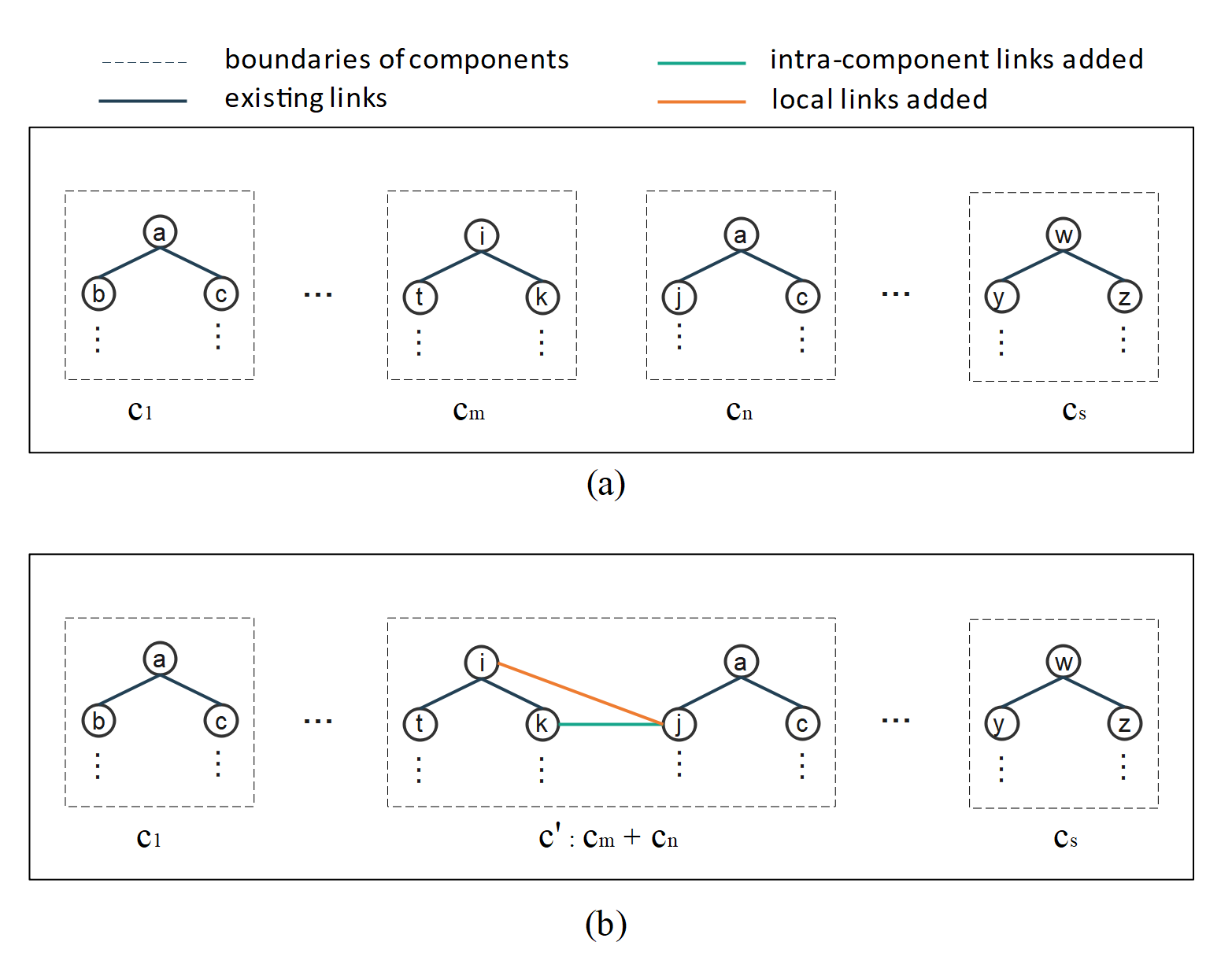
Figure 2 shows an example of an attacked network consisting of non-empty components $\mathcal{C}=\{c_{1},\dots,c_{s}\}$ , where each component consists of a connected subgraph. Let vertices $i$ and $k$ belong to vertices of component $c_{m}$ , ( $i,k\in V(c_{m})$ ), and vertex $j$ belongs to vertices of component $c_{n}$ ( $j\in V(c_{n}))$ . There are two candidates for intra-component links as $y^{R}_{ij}$ and $y^{R}_{kj}$ . Assuming we first add intra-component link $y^{R}_{kj}$ connecting components $c_{m}$ and $c_{n}$ , the resulting component becomes a larger component $c^{\prime}=c_{m}+c_{n}$ . Therefore, since all vertices of $c_{m}$ and $c_{n}$ are now unified in component $c^{\prime}$ , link $y^{R}_{ij}$ becomes a local link for the new component $c^{\prime}$ , and as shown before, adding a local link would not improve the network connectivity anymore. In other words, from the network connectivity point of view, adding multiple intra-component links between two given components has the same impact on the rupture degree as adding only one intra-component link between the two components. It is because the purpose of link addition is to connect two individual components so that there exists a path between any vertex of the first component and any vertex of the second component. Thus, even though adding multiple intra-component links provides multiple such paths, it does not change the rupture degree which is mainly measured by the number of vertices in the largest component. Therefore, for every two components, all the candidate intra-component links between them have the same value for improving network connectivity but may have different financial values and costs. Thus, to find the optimal solution of the response problem, it is sufficient to consider only the most cost-efficient intra-component (MCEIC) links, i.e., the cheapest links, between any two components, one link per two components, to be the candidate links in the response problem. In particular, if we choose to connect two components $i$ and $j$ , there is only one candidate MCEIC link between the components which can be added. Doing so, the response problem reduces to a problem determining which MCEIC links should be selected to maximize network resilience given a budget constraint.

To set up an equivalent problem to the response problem, let $d_{ij}$ be the cost of adding an intra-component link between vertex $i\in V(c_{m})$ and vertex $j\in V(c_{n})$ . Letting

\underline{d}_{mn}=\min_{\begin{subarray}{c}i\in V(c_{m})\\ j\in V(c_{n})\end{subarray}}\{d_{ij}\},\qquad\forall m,n\in\mathcal{C}^{R}=\{1,\dots,s\}

(15)

symmetric matrix $\underline{\mathbf{d}}$ is the min-cost matrix and finds the minimum cost of adding any two components using the MCEIC link between the two components. Also, let $x_{mn}\in\{0,1\}$ be a vector of binary variables indicating 1 if MCEIC link between two components $c_{m}$ and $c_{n}$ is added in the reconstructed network. The following proposition shows the response problem reduces to an equivalent problem (16).

Proposition 4.9

The response problem 7 is equivalent to


$\displaystyle-\|X\|\hskip 2.84544pt+\hskip 2.84544pt\min_{\mathbf{x},\mathbf{t},\alpha^{R}}\quad$	$\displaystyle\Big(-\alpha^{R}+{\|\mathcal{C}^{R}\|-\sum_{m\in\mathcal{C}^{R}}\sum_{\begin{subarray}{c}n\in\mathcal{C}^{R}\\ n>m\end{subarray}}x_{mn}}+\epsilon\sum_{m\in\mathcal{C}^{R}}t^{R}_{m}\Big)$		(16a)
	$\displaystyle\sum_{m\in\mathcal{C}^{R}}t^{R}_{m}\geq 1$		(16b)
	$\displaystyle\|V(c_{m})\|+\sum_{\begin{subarray}{c}n\in\mathcal{C}^{R}\\ n\neq m\end{subarray}}\|V(c_{n})\|x_{mn}\leq\alpha^{R}\leq\|V(c_{m})\|+\sum_{\begin{subarray}{c}n\in\mathcal{C}^{R}\\ n\neq m\end{subarray}}\|V(c_{n})\|x_{mn}+M(1-t^{R}_{m})$	$\displaystyle\forall m\in\mathcal{C}^{R}$	(16c)
	$\displaystyle\sum_{m\in\mathcal{C}^{R}}\sum_{\begin{subarray}{c}n\in\mathcal{C}^{R}\\ n>m\end{subarray}}\underline{d}_{mn}x_{mn}\leq B^{R}$		(16d)
	$\displaystyle x_{mn}=x_{nm}\hskip 227.62204pt\forall m,n\in\mathcal{C}^{R}$		(16e)
	$\displaystyle\mathbf{x}\in\{0,1\}^{\|\mathcal{C}^{R}\|^{2}},\mathbf{t}\in\{0,1\}^{\|\mathcal{C}^{R}\|},\alpha^{R}\in\mathbb{R}_{+}$		(16f)

where $|X|=(|\mathcal{N}|-\sum_{i\in\mathcal{N}}\sum_{c\in\mathcal{C}}v^{A*}_{ic})$ is the size of the worst cut set which was identified in the attack problem.

Proof 4.10

Proof. Constraints (7d), (7h)-(7l) of response problem 7 correspond to the structure of components to ensure only intra-component links can be added in the reconstructed network. It easily follows that these constraints are all implied in Formulation (16) using the definition of MCEIC links. Also, to find the number of components, we know each MCEIC link unifies two components and thus reduces the number of components by 1. Therefore, $(|\mathcal{S}|-\sum_{m\in\mathcal{S}}\sum_{\begin{subarray}{c}n\in\mathcal{S}\\ n>m\end{subarray}}x_{mn})$ corresponds to the number of components after link addition, which is considered in the objective function, and implies that constraint (7e) is not necessary anymore. Furthermore, allowing the MCEIC links to be the only candidate links in the attack problem, constraints (7c), (7b), (7f), (7g) of the response problem correspond to (16b), (16c), (16d), (16e), respectively. In addition, after relaxing restrictions on $\alpha$ (based on Proposition 4.7), constraint (8) reduces to (16f). $\square$

Given the optimal solution of (16), one can find the intra-component links added to the reconstructed network ( $\mathbf{y}^{R}$ ), the length of the largest component ( $\alpha^{R}$ ), the number of components, and thus, the optimal value of network resilience under the worst-case attack. It is to be note Formulation (16) is less complicated than the response problem 7 and has significantly a less number of constraints and integer variables, and thus is expected to be computationally less challenging. Furthermore, we can show that there exists an embedded knapsack constraint in problem 16 for which we can generate LCIs so that solving formulation 16 becomes even more time-efficient. To do so, we first present a simple re-indexing procedure to convert two-dimensional matrices into vectors, which can be done in polynomial time.

4.4.1 Re-indexing Procedure

In Formulation 16, matrix variable $\mathbf{x}$ is a two-dimensional symmetric matrix where $x_{mn}=x_{nm}$ and $x_{nn}=0,\forall m,n\in\{1,\dots,s\}$ . Let $|\mathcal{C}^{R}|=s$ . To identify the underlying knapsack constraint from Formulation 16, it is sufficient to take into consideration the upper triangular matrix $\mathbf{x}$ which has $s(s-1)/2$ elements, instead of considering $s^{2}$ elements in matrix $\mathbf{x}$ . Then, we store all elements of upper triangular matrix $\mathbf{x}$ in a vector $\hat{x}$ .

Figure 3 shows the re-indexing and mapping from matrix $\mathbf{x}$ to vector $\hat{\mathbf{x}}$ . Particularly, we place all rows of matrix $\mathbf{x}$ in vector $\hat{\mathbf{x}}$ where row $m$ of matrix $\mathbf{x}$ starts at position $S_{I}(m)=1+\sum_{k=1}^{m-1}(s-k)$ of vector $\hat{\mathbf{x}}$ . Therefore, considering any element $x_{mn}$ in the upper triangular matrix $\mathbf{x}$ ( $m<n$ ), this element is mapped to the $\sigma(m,n)$ -th element of vector $\hat{\mathbf{x}}$ , denoted by $\hat{x}_{\sigma(m,n)}$ , where

\displaystyle\sigma(m,n)=(n-m)+\sum_{k=1}^{m-1}(s-k)

(17)

Given this re-indexing, for example $\sum_{\begin{subarray}{c}n\in\mathcal{C}^{R}\\ n\neq m\end{subarray}}|V(c_{n})|x_{mn},\forall m\in\mathcal{C}^{R}$ in (16c) can be re-written as follows

\sum_{n=1}^{m-1}|V(c_{n})|\hat{x}_{\sigma(n,m)}+\sum_{n=m+1}^{s}|V(c_{n})|\hat{x}_{\sigma(m,n)}\qquad\quad\forall m\in\mathcal{C}^{R}

(18)

Similarly, let vector $\tilde{\mathbf{d}}$ be a cost vector with the same size as vector $\hat{x}$ where $\tilde{\mathbf{d}}=\{\underline{d}_{12},\dots,\underline{d}_{1s},\dots,\underline{d}_{rs}\dots,\underline{d}_{(s-1)s}\}$ , implying that the cost of adding a MCEIC link between components $m$ and $n$ is stored in $\tilde{d}_{z}$ where $z=\sigma(m,n)$ . Thus, given the re-indexing procedure, the Formulation 16 reduces to Formulation 19.


$\displaystyle-\|X\|+\min_{\hat{\mathbf{x}},\mathbf{t},\alpha^{R}}\quad$	$\displaystyle-\alpha^{R}+(\|\mathcal{S}\|-\sum_{z=1}^{s(s-1)/2}\hat{x}_{z})-\epsilon\sum_{m\in\mathcal{S}}t^{R}_{m}$		(19a)
	$\displaystyle\sum_{m=1}^{s}t^{R}_{m}\geq 1$		(19b)
	$\displaystyle\|V(c_{m})\|+\sum_{n=1}^{m-1}\|V(c_{n})\|\hat{x}_{\sigma(n,m)}+\sum_{n=m+1}^{s}\|V(c_{n})\|\hat{x}_{\sigma(m,n)}\leq\alpha^{R}$
	$\displaystyle\leq\|V(c_{m})\|+\sum_{n=1}^{m-1}\|V(c_{n})\|\hat{x}_{\sigma(n,m)}+\sum_{n=m+1}^{\|\mathcal{S}\|}\|V(c_{n})\|\hat{x}_{\sigma(m,n)}+M(1-t^{R}_{c})$	$\displaystyle\forall m\in\mathcal{C}^{R}$	(19c)
	$\displaystyle\sum_{z=1}^{s(s-1)/2}\underline{d}_{z}\hat{x}_{z}\leq B^{R}$		(19d)
	$\displaystyle\hat{\mathbf{x}}\in\{0,1\}^{s(s-1)/2},\mathbf{t}\in\{0,1\}^{s},\alpha^{R}\in\mathbb{R}_{+}$		(19e)

Formulation 19 is a smaller problem than Formulation 16 due to reducing the number of variables and constraints by the re-indexing procedure. Furthermore, constraint (19d) corresponds to a knapsack constraint for which we derive LCIs based on Letchford and Souli 2019, to reduce the computational challenges. As a result, instead of the response problem 7, one can solve Formulation 19 which is time-efficient while providing the same global optimal solution.

4.5 Extension to Other Types of Attacks

There are several types of attacks studied in the literature of network resilience and robustness. A common approach is to identify the worst-case attack and optimize the network under such attacks as it was shown that cascading failures are mainly due to targeted attacks (Ruj and Pal 2014).

However, there are other types of attacks or failures in various networks. For instance, in several networks, such as power system networks or supply chain networks, the random failure of nodes plays an important role in network non-resilience due to the probabilistic age function of equipment, natural disasters, etc. (Sadrabadi et al. 2021, Ji et al. 2016). We refer to such failures as random attacks. Furthermore, in some cases, the attackers desire to disable a set of certain nodes, not necessarily the most critical nodes, in a network due to geographical location, importance, political reasons, etc. We refer to such attacks as designated attacks. Finally, in some networks, the nodes can be divided into some subgroups where the attacker is interested in attacking certain subgroups based on their properties. For example, the nodes of a power system network can be divided into generation and load nodes, where if the generation nodes are disabled, the load nodes cannot be supplied automatically. Thus, the attacker might be interested in disabling the generation nodes to cut the power supply. We refer to this type of attack as distributed attacks.

4.5.1 Random and Designated Attacks

In the case of having random, one needs to determine the set of nodes that are most likely to be attacked before optimizing the network resilience. Such analysis can be done using probabilistic evaluation based on the failure distributions of nodes, Monte Carlo simulation, Markov Chain models, etc. Similarly, in case of having designated attacks, the nodes that are subject to attack are known in advance.

Let $X^{\text{n}}$ be the cut set corresponding to the random or designated attacks. If $G(V-X^{\text{n}})$ is a connected graph, there is a path between any two nodes of the attacked network and all the remaining nodes are able to communicate. Thus, the network resilience is maximized. However, if $G(V-X^{\text{n}})$ is not connected, once can apply the proposed framework to maximize network resilience. Since these cut sets are known or estimated in advance, the network resilience is to be maximized under such cut sets, as opposed to the worst cut set. Thus, the attack problem is not needed to be solved anymore. As a result, our proposed two-stage formulation reduces to only the response stage where the network resilience is aimed to be maximized under a pre-identified cut set. By letting $X=X^{\text{rand}}$ or $X=X^{\text{d}}$ in the response problem, our proposed approach is able to optimize network resilience for random or designated attacks.

4.5.2 Distributed Attacks

In the case of having distributed attacks, one needs to classify each node of a network in subsets of nodes considering a certain property of interest. Without loss of generality, we divide the nodes in two subsets and it can be extended to more subsets. Consider a network with a set of nodes denoted by $\mathcal{N}$ . Let $\mathcal{N}_{I}$ and $\mathcal{N}_{J}$ be two subsets of $\mathcal{N}$ such that $\mathcal{N}_{I}\cap\mathcal{N}_{J}=\emptyset$ and $\mathcal{N}_{I}\cup\mathcal{N}_{J}=\mathcal{N}$ . Supposing the attacker is interested in only disabling the nodes of subset $\mathcal{N}_{I}$ . Thus, Constraint 4b is re-written as follows:


$\displaystyle\sum_{c\in\mathcal{C}}v^{A}_{ic}\leq 1$	$\displaystyle\forall i\in\mathcal{N}_{I}$	(20a)
$\displaystyle\sum_{c\in\mathcal{C}}v^{A}_{ic}=1$	$\displaystyle\forall i\in\mathcal{N}_{J}$	(20b)

where Constraint (21a) allows the possibility of disabling each vertex $i\in\mathcal{N}_{I}$ by the worst-case attack. Otherwise, the vertex remains active and is at most in one component. Also, Constraint (21b) enforces that all vertices of subset $\mathcal{N}_{J}$ remain active after the attack and belong to exactly one component after the worst-case attack. This reformulation can also be used for the type of attacks mentioned in Abbas et al. 2017 where a subset of nodes always remain intact and cannot be disabled. The rest of the proposed two-stage model remains the same as before and one can use the proposed solution method to address the network resilience and robustness under such distributed attacks.

5 Numerical Results

In this section, we first provide a illustrative numerical example to show the benefits of our methodology in terms of network resilience and robustness and the effects of the budget on the link addition strategies. Then, we use larger problems to demonstrate the computational benefits of the proposed solution method. In all numerical examples, we generate random connected graphs and execute the proposed algorithm. For all instances, we let the cost for attacking each node be 1 unit and the total budget for attack be $|\mathcal{N}|/2$ units so that no more than half of the nodes are allowed to be disabled in the attack stage. All instances are performed using the MIP solver of Gurobi Version 9.1 on a 1.5 GHz×86 laptop with 1GB main memory, and the optimality gap is set to 0 for all instances.

5.1 Resilience and Robustness Analysis

In this section, we present a network with 9 vertices and 9 edges, shown in Figure 4.(a), to demonstrate the benefits of the proposed network. Solving the attack problem, the worst cut set is $X=\{5\}$ corresponding to the lowest network resilience ( $-r_{X}(G)$ ). This implies the connectivity of this network heavily relies on vertex 5. Therefore, the worst-case attack can occur by disabling vertex 5. Figure 4.(b) shows the structure of the network under the worst-case attack by removing vertex 5. Since there exist 5 components in Figure 4.(b), one can interpret that the maximum network resilience can be obtained by adding 4 intra-component links, if the link addition budget allows. It is because once all 5 components are connected together using 4 intra-component links, the resulting network consists of only one component. Figure 4.(c) shows the reconstructed network under the worst-case attack which consists of the original network and the new intra-component links added to the network. For now, we do not consider the budget constraint for link addition. The green links are those added to maximize the network resilience under the worst-case attack to reduce the dependencies on vertex 5 so that the remaining vertices are able to properly communicate in the absence of vertex 5.

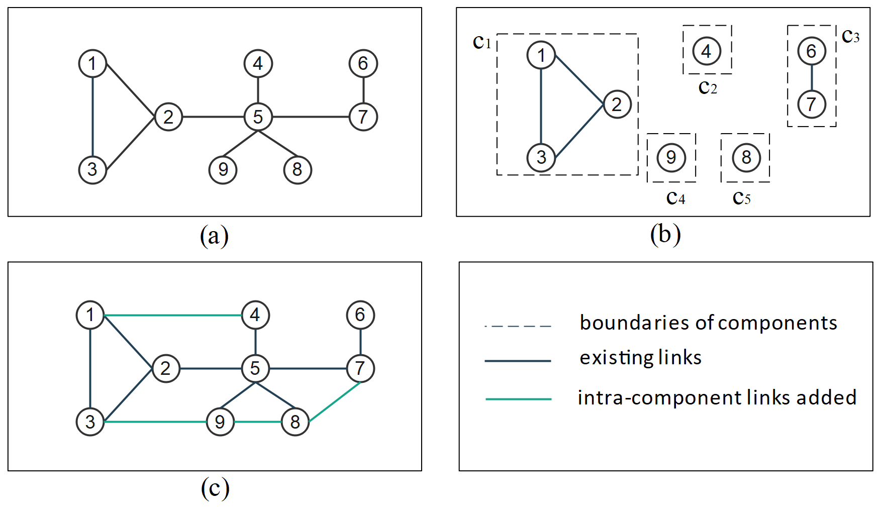
In Table 1, we manually choose a number of cut sets $X_{i}$ s, not necessarily the worst cut set, and measure the network resilience of the initial network, denoted by $-r_{X}(G)$ and that of the reconstructed network, denoted by $-r^{R}_{X}(G)$ . As observed, in the initial network, $X_{1}=\{5\}$ is the worst cut set corresponding to the lowest value of the network resilience which shows the network is more vulnerable and can seriously be damaged in the absence of vertex 5. For other cut sets, the network is more resilient as $-r_{X_{1}}(G)=-1\leq-r_{X_{i}}(G),\forall i\neq 1$ , implying either the network is less dependent on the vertices of other cut sets or there is more work required to damage the network by disabling more vertices of a cut set.

Table 1: Resilience and Robustness analysis for different cut sets of the initial and the reconstructed network

	Initial Network		Reconstructed Network
Cut set	# of components	$\text{NR}:-r_{X}(G)$	# of components	$\text{NR}:-r^{R}_{X}(G)$
$X_{1}=\{5\}$	5	-1 $(r^{*})$	1	8
$X_{2}=\{2\}$	3	5	1	8
$X_{3}=\{5,7\}$	4	0	2	6
$X_{5}=\{2,5,7\}$	5	0	2	6
$X_{4}=\{2,5,8\}$	4	1	2	5
$X_{5}=\{2,5,7,9\}$	4	2	3	4
$X_{6}=\{1,2,5,9\}$	5	2	3	4
$X_{7}=\{1,2,5,8\}$	4	2	3	3
$X_{8}=\{1,2,5,7,9\}$	4	2	4	2 $(r^{R*})$
$X_{9}=\{3,2,5,7,9\}$	4	2	3	4
NR: Network Resilience
*: optimal objective value of the attack problem

From Table 1, there are three main observations on the reconstructed network, which are obtained after immunizing the network against the worst-case attack. First, the network resilience for $X_{1}=\{5\}$ significantly improves from $-1$ to $8$ after we add links meaning that the functionality of the reconstructed network does not heavily depend on only vertex 5. Thus, if vertex $5$ is damaged, the rest of the network is able to maintain its proper functioning and communication with other parts of the network. Therefore, the reconstructed network is more resilient in the absence of the worst-case attack. Second, after adding links to the initial network, the network dependencies on only vertex 5 decrease. Thus, the new worst cut set in the reconstructed network may consist of other vertices along with vertex 5. We call this dynamic worst cut set since it is obtained after the link addition strategies are known. In particular, the cut set $X_{8}=\{1,2,5,7,9\}$ becomes the dynamic worst cut set for the reconstructed network. This means that after links are added to the network, the most severe damage to the reconstructed network occurs only when all vertices 1, 2, 5, 7, and 9 are simultaneously disabled. We refer to this as the network robustness measured by the size of the worst cut set. Thus, by adding links, the network robustness increases from $|X_{1}|=1$ to $|X_{8}|=5$ implying that disabling all these five vertices simultaneously requires more budget and more work done to damage the network, which might not be a viable option for the attacker due to the budget constraint considered in the attack problem. Third, assuming the attacker can dynamically respond to our link addition actions and has enough budget to disables all vertices of cut set $X_{8}$ , we observe that the network resilience for the reconstructed network under the new (dynamic) worst-case attack is more than that of the initial network, i.e., $r^{*}=-1<r^{R*}=2$ . This shows that the reconstructed network not only is significantly more resilient against the worst cut set of the initial network, i.e., $X_{1}$ , but also it becomes more resilient against the dynamic worst cut set of the reconstructed network, i.e., $X_{8}$ , that may be identified if the attackers can dynamically change their decisions based on our link addition strategy. The mentioned observations demonstrate how the proposed approach leads to a reconstructed network that is both more resilient and robust against the initial and dynamic worst-case attacks.

5.2 Effects of the link addition budget

In this section, we show the effects of the budget considered for link addition on the network resilience and robustness. To do so, we first find the matrix $\underline{\mathbf{d}}$ obtained from (15) to find all candidate MCEIC links of the attacked network considered in Figure 4.b. The cost of adding MCEICs link and the two ends of such links, presented in parenthesis, are shown in (5.2).

\underline{\mathbf{d}}=\begin{array}[]{cccccc}c_{1}&c_{2}&c_{3}&c_{4}&c_{5}\\ -&1.5(1\textendash 4)&2.2(2\textendash 7)&1.5(3\textendash 9)&1.6(2\textendash 8)&c_{1}\\ &-&1.8(4\textendash 6)&2.2(4\textendash 9)&2.2(4\textendash 8)&c_{2}\\ &&-&2.3(7\textendash 9)&1.3(7\textendash 8)&c_{3}\\ &&&-&1.0(8\textendash 9)&c_{4}\\ &&&&-&c_{5}\\ \end{array}

Figure 5: Network resilience (shown by the left vertical axis) and robustness (shown by the right vertical axis) for different values of link addition budgets. Shaded areas correspond to various ranges of the budget with a constant number of links added where the brightest area has 0 links, the darkest area has 4 links, and the increment is 1 link.

After the worst attack $X_{1}=\{5\}$ is identified, one can maximize the network resilience by link addition within a budget so that the network maintains a maximum functionality level in the absence of node $5$ . However, when the budget is limited, one cannot connect all the remaining components. Thus, the best combination of the intra-component links should be selected to maximize the network resilience within the budget. In addition, as we showed, the link addition reduces the dependencies on the worst cut set $X_{1}=\{5\}$ , and includes more vertices in the new cut set for the reconstructed network. Thus, we expect to have larger cut sets (higher robustness) when more intra-component links are added to the network.

Figure 5 demonstrates the effects of link addition budget on the reconstructed network under the initial worst-case attack $X_{1}=\{5\}$ . The network resilience (measured by $-r_{X_{1}}^{R}(G)$ and shown by the left vertical axis) and the network robustness (measure by $|X^{*}|$ and shown by the right vertical axis) for various values of the budget assigned for the link addition. In the figure, shaded areas correspond to various ranges of the budget within which a constant number of links is added, where the brightest area on the left indicates 0 links are added in the reconstructed network, the darkest area indicates 4 links are added in the reconstructed network, and the increment is 1 link. For example, $2.5\leq B^{R}<3.8$ corresponds to the third shaded area where two MCEIC links are added to the reconstructed network. From the figure, it is observed that once the budget is less than 1, no MCEIC link is added in the repair stage since the budget is not enough. Thus, the reconstructed network is equivalent to the initial network with $-r^{R}_{X_{1}}(G)=-1$ . However, as the budget increases, the best MCEIC link candidates given different levels of the budget are added to the network which corresponds to a higher value for $-r^{R}_{X_{1}}(G)$ , which in turn enhances the network resilience under the initial worst-case attack. For example, when the budget is $1.3$ units, the only MCEIC link that can be added is link $7$ - $8$ , which unifies components $c_{3}$ and $c_{5}$ (decreases the number of components by 1) without changing the largest component $c_{1}$ . Thus, $-r^{R}_{X_{1}}(G)=0$ . However, when the budget increases to 1.5, the response problem allows to add MCEIC link $1$ - $4$ , instead of link $7$ - $8$ , since the new link connects components $c_{1}$ and $c_{3}$ (drops the number of components by 1) while increasing the length of the largest component $c_{1}$ by 1. Thus, $-r^{R}_{X_{1}}(G)=1$ . By further changing the budget assigned for link addition, the optimal topology of the reconstructed network changes with objective to increase the network resilience. Finally, once there is sufficient budget (i.e., any budget greater than 5.3 units), 4 MCEIC links are added to the network to unify all components resulting in maximum resilience, which corresponds to the solution of the previous part where we ignored the budget constraint.

The secondary axis of Figure 5 evaluates the network robustness $|X^{*}|$ of the reconstructed network for various levels of the budget. To evaluate the network robustness, we dynamically find the new worst cut sets of the reconstructed network, as the dependencies may change once new links are added. For the initial network, $|X^{*}|=1$ , meaning that by removing one vertex the network experiences the more severe damage. However, as the budget increases the reconstructed network becomes more robust so that one may need to disable more number of vertices to severely damage the network, which might not be an affordable option for the attacker. Ultimately, once there is a sufficient budget, i.e., $B^{R}\geq 5.3$ , the dynamic worst cut set includes five vertices implying that damaging the network is more difficult since all five vertices should be simultaneously disabled. The mentioned analyses provide an intuitive picture for the managers to determine the desired level of robustness and resiliency that they would like to consider within a financial budget.

5.3 Computational and Robustness Analysis

In this section, we further evaluate the performance of the proposed framework, mostly focusing on the computational results. We randomly generate 14 instances to execute the proposed framework¹¹ 1 the data for the random instances are available at https://github.com/miladdf94/Network-resilience/blob/main/Adj.%20matrix%20-%20instances.txt. In our implementation, we relax the link addition budget constraint (in the response problem) to let the proposed framework maximizes the network resilience without financial limitations.

Table 2 and 3, respectively, show the resilience and robustness results as well as computational results for 14 randomly-generated instances. From Table 2, it can be observed that:

•

For all instances, the network robustness noticeably increases, where $|X^{*}|$ and $|X^{{}^{\prime}*}|$ measure the robustness of the initial and the reconstructed networks. In particular, for instance #1, $|X^{*}|$ and $|X^{{}^{\prime}*}|$ are 3 and 6, respectively, implying that the most severe damage in the initial network occurs when 3 vertices are attacked simultaneously, while to most severely attack the reconstructed network, 6 vertices are required to be disabled simultaneously.
•

In all instances, the reconstructed network is significantly more resilient against the initial worst-case attack (denoted by $-r^{R}_{X^{*}}(G)$ ) compared to the initial network (denoted by $-r_{X^{*}}(G)$ ). In addition, if the attacker has the ability to change its decisions based on the link addition strategy in the response stage, the new worst-case attack is denoted by $X^{{}^{\prime}*}$ , which is impacted by the new links added to the initial network. It can be observed that in such a case, the network resilience in the reconstructed network is still significantly higher than that of the initial network, i.e., $-r_{X^{*}}(G)<-r^{R}_{X^{{}^{\prime}*}}(G)$ for all instances, demonstrating the benefits of the proposed framework both for static and dynamic worst-case attacks.

Also, Table 3 presents the computational results of the mentioned instances. We first solve the proposed two-stage model directly in Gurobi, and then implement our proposed solution method and solve the two-stage model in Gurobi. In Table 3, column ”solver cut” corresponds to the number of cuts generated in Gurobi, and ”add. user cuts” indicated the number of additional LCI cuts (Letchford and Souli 2019) that we manually added to the solver cuts to solve the attack problem. Also, ”nodes” corresponds to the number of nodes (branches) that are explored in the branch-and-bound (B&B) algorithm to find the optimal solution. For the response problem, we did not add LCI cuts since we relaxed the link addition budget constraint to more clearly demonstrate the performance of the proposed method.

From Table 3, it can be observed that the proposed solution method significantly reduces the solve time by exploiting the problem structure. For the attack problem, the proposed approach solves the attack problem faster and more efficiently. This is due to the efficient relaxation in the proposed approach as well as the LCIs added to the attack problem. On the other hand, in the response stage, the proposed approach corresponds to a much simpler, but equivalent, problem that can be solved faster than the original response problem. In particular, our proposed solution method requires exploring 1 node in the B&B algorithm to find the optimal solution. However, without implementing the proposed algorithm, the B&B algorithm exhaustively explores a large number of nodes to find the optimal solution. The mentioned observations validate the benefits of the proposed solution method from the resilience and robustness point of view as well as computational aspects.

Table 2: Resilience and Robustness analysis of initial and the reconstructed network for various instances

	# of	# of	Used	# of MCEIC	Initial network		reconstructed network
Instance	nodes	edges	budget	links	$\|X^{*}\|$	$-r_{X^{*}}(G)$	$-r_{X^{*}}^{R}(G)$	$\|X^{{}^{\prime}*}\|$	$-r_{X^{{}^{\prime}*}}^{R}(G)$
1	11	15	5.55	4	3	0	10	6	6
2	11	20	6.95	4	5	2	10	6	6
3	12	20	6.70	5	5	1	11	6	6
4	12	30	4.50	3	6	4	11	7	7
5	15	19	14.05	8	5	-2	14	6	6
6	15	26	12.05	6	7	2	14	8	8
7	16	20	9.05	7	5	-1	15	7	7
8	16	32	7.50	5	7	3	15	8	8
9	17	21	11.40	8	6	-1	16	7	2
10	17	30	9.65	7	7	1	16	9	9
11	18	19	12.25	8	5	-2	17	7	7
12	18	25	13.75	8	6	-1	17	8	8
13	21	25	14.10	10	7	-2	21	8	8
14	22	27	11.75	10	7	-2	21	9	9

Table 3: Computational analysis of initial and the reconstructed network for various instances

	without the proposed solution method						with the proposed solution method
	Attack problem			Response problem		Total	Attack problem			Response problem		Total
Instance	solver cuts	nodes	time (s)	nodes	time (s)	time (s)	add. user cuts	nodes	time (s)	nodes	time (s)	time (s)
1	120	3723	2.14	8	0.12	2.26	14	786	0.98	1	0.03	1.01
2	129	4665	2.64	156	0.14	2.79	11	937	1.10	1	0.02	1.12
3	143	3613	3.26	206	0.14	3.40	19	704	0.93	1	0.02	0.95
4	98	10757	5.69	675	0.28	5.96	7	1589	1.92	1	0.03	1.95
5	248	8374	6.80	5093	2.13	8.93	18	1396	1.74	1	0.03	1.77
6	728	118584	60.21	12034	7.07	67.29	35	60543	36.10	1	0.03	36.13
7	523	40959	27.15	798	4.15	31.31	22	34367	25.19	1	0.03	25.22
8	451	281822	177.78	23092	12.06	189.54	81	116553	89.20	1	0.02	89.21
9	750	157823	91.25	16798	11.16	102.41	64	74979	51.47	1	0.01	51.49
10	663	131102	103.38	12489	9.09	112.47	14	57593	54.62	1	0.01	54.63
11	329	3827887	1416.52	78920	28.98	1445.50	103	1975251	857.02	1	0.01	857.03
12	1264	197532	273.95	34952	19.53	293.48	76	169814	259.89	1	0.39	260.28
13	468	2602844	2452.91	98204	48.79	2501.70	112	1311943	1454.68	1	0.20	1454.88
14	299	3958319	2835.65	112485	98.08	2933.73	187	1755735	1666.87	1	0.30	1667.16
Average	443	810572	532.79	28279	17.27	550.06	54	397298	321.55	1	0.08	321.63
add. user cuts: additional user cuts

5.4 Application to Power System Networks

Reliability concerns have been one of the main focuses of researchers in power system networks since 1960s (Billinton and Bollinger 1968, Nazemi and Mashayekhi 2014), and has been constantly the topic of recent studies from various aspects (Panteli et al. 2017, Fathabad et al. 2020). Depending on the location of generators in a power system, the nodes of a power system network can be categorized into generation nodes, load nodes, and hub nodes, i.e., main substations used to transfer power to various points of the system. From the service reliability point of view, the generation nodes are the most important ones since a failure in generation nodes interrupts the supply and results in a blackout at load points. Also, hub nodes are of special interest since they are larger stations to distribute power in smaller areas. The rest of the nodes are mainly load nodes which are not as important as the other groups from the reliability point of view because the power outage usually occurs due to the failure in generation nodes or hub nodes that are used for power distribution. As result, one may be interested in enhancing the power system reliability while considering distributed attacks, e.g., letting the possibility of failure only for the generation and hub nodes.

In this section, we demonstrate the applicability of the proposed approach in the IEEE 14 Bus Test system representing a portion of the American Electric Power System in the Midwestern US (Christie 2000). Figures 6 and 7.a show the actual IEEE 14-Bus system and the underlying graph for the system, where we categorize the buses in 3 groups, namely (i) $\mathcal{N}_{g}=\{1,2,3,6,8\}$ , corresponding to generator nodes, (ii) $\mathcal{N}_{h}=\{4,5,9\}$ , corresponding to hub nodes, and (iii) $\mathcal{N}_{i}=\{7,10,11,12,13,14\}$ , corresponding to the rest of nodes that are considered intact in this example.

In such power systems, we consider distributed attacks discussed in section 4.5.2, where in the attack problem nodes in $\mathcal{N}_{i}$ are intact. As a result, Constraint 4b is replaced by the following constraints


$\displaystyle\sum_{c\in\mathcal{C}}v^{A}_{ic}\leq 1$	$\displaystyle\forall i\in\mathcal{N}_{g}\cup\mathcal{N}_{h}$	(21a)
$\displaystyle\sum_{c\in\mathcal{C}}v^{A}_{ic}=1$	$\displaystyle\forall i\in\mathcal{N}_{i}$	(21b)

to ensure that all vertices of subset $\mathcal{N}_{i}$ remain intact since they are not of the attacker’s interest. Figure 7.b corresponds to the solution of the attack problem where the worst cut set is $|X|=\{2,4,6.9\}$ corresponding to the minimum resilience of $r^{*}(G)=1$ . It can be observed that components such as $c_{1}$ and $c_{2}$ only contains load nodes while some components may contain generation nodes as well as other types of nodes.

In the response stage, one may consider the technical characteristics of the power system prior to adding links. In particular, one can argue that even though linking components $c_{1}$ and $c_{2}$ increases the network resilience due to a higher level of connectivity, this connection might not be beneficial from the service reliability point of view. It is because all nodes of components $c_{1}$ and $c_{2}$ are load nodes, and such load nodes cannot be supplied in the absence of $|X|=\{2,4,6.9\}$ . Therefore, the connection of components $c_{1}$ and $c_{2}$ in the response stage is reasonable only if other components with generation nodes are also connected to components $c_{1}$ or $c_{2}$ . Let $\mathcal{C}_{l}$ be the set of components whose nodes are all load nodes and $\mathcal{C}_{g}$ be the set of components that have at least 1 generator. To impose such technical constraints, we extend the response problem for power system networks by adding the following constraint.

\hat{x}_{\sigma(m,n)}\leq\sum_{i\in\mathcal{C}_{g}}\big(\hat{x}_{\sigma(m,i)}+\hat{x}_{\sigma(n,i)}\big)\qquad\forall m,n\in\mathcal{C}_{l}

(22)

where $\hat{x}_{\sigma(m,n)}$ is a binary variable indicating if a MCEIC link between components $m$ an $n$ is added. Constraint 22 enforces that if a MCEIC link connects load components $m,n\in\mathcal{C}_{l}$ , there should also exists at least one MCEIC link connecting a component with generators to one of the load components $m$ or $n$ . As a result, the power system resilience is optimized with respect to power reliability indices as well rather than merely considering the graph topological properties.

In addition, in the response stage, various indices can be used to calculate matrix $\underline{\mathbf{d}}$ for MCEIC to be considered in the response problem. For example, one may consider the installation cost of MCEIC links as well as the reduced interrupted cost as a resulting of connecting two components. For example from Figure 7.b, once load component $c_{1}$ is connected to component $c_{3}$ with generator, it is expected that generator located at node 1 transfers power to supply nodes of component $c_{1}$ . Thus, this link addition is more beneficial, and as a result one can consider a low value in matrix $\underline{\mathbf{d}}$ for the MCEIC link connecting components $c_{1}$ and $c_{3}$ . We form matrix $\underline{\mathbf{d}}$ as the installation cost minus the potential reduction in the interrupted cost of the load nodes. In other words, matrix $\underline{\mathbf{d}}$ represents the financial benefits of the MCEIC links. For example, link $e_{1}$ = $12$ - $1$ is more beneficial than $e_{2}$ = $1$ - $11$ because $e_{1}$ can potentially lead to supplying 3 load nodes of $c_{1}$ , i.e., nodes 12, 13, 14, and reduce the interruption cost more. However, $e_{2}$ can reduce the interruption cost of only two load nodes located in $c_{2}$ , i.e., nodes 10, 11. Matrix $\underline{\mathbf{d}}$ used in the second stage is formed as follows:

\underline{\mathbf{d}}=\begin{array}[]{cccccc}c_{1}&c_{2}&c_{3}&c_{4}&c_{5}\\ -&2.8(14\textendash 10)&1.4(12\textendash 1)&1.7(14\textendash 3)&1.5(14\textendash 7)&c_{1}\\ &-&1.8(1\textendash 11)&1.8(10\textendash 3)&1.7(11\textendash 8)&c_{2}\\ &&-&2.1(5\textendash 3)&1.8(5\textendash 7)&c_{3}\\ &&&-&1.7(3\textendash 8)&c_{4}\\ &&&&-&c_{5}\\ \end{array}

Figure 7 corresponds to the reconstructed network given the available budget for the link addition is 3 units, i.e., $B^{R}=3$ . It is observed that two links can be added in the reconstructed network. Table 4 summarizes the results for the IEEE 14 Bus test system. It is observed that $X_{1}=\{2,4,6,9\}$ correspond to the lowest resilience, i.e., $-r^{*}_{X_{1}}(G)=1$ , in the initial network before link addition. Once, links $e_{1}$ and $e_{2}$ are added to the network, the network resilience under the same cut set $X_{1}$ enhances to $-r^{R}_{X_{1}}(G)=7$ , implying the system is more resilient under attacks. Furthermore, in the reconstructed network, set $X_{2}=\{1,2,6,9\}\subset\mathcal{N}_{h}\cup\mathcal{N}_{g}$ becomes the new worst cut set as the dependencies in the reconstructed network change after link addition. Thus, if the attacker has the ability to dynamically respond to our link addition actions, the attacker may choose to disable vertices of $X_{2}$ resulting in the lowest resilience in the reconstructed network, i.e., $-r^{R*}_{X_{2}}(G)=5$ . However, it is obvious that the reconstructed network is significantly more resilient even under the new (dynamic) worst-case attack, compared to the initial network. The mentioned observations validate the benefits of the proposed solution for enhancing networks resilience and robustness in power system networks.

Table 4: Resilience and Robustness analysis of the IEEE 14 Bust Test System for

B^{R}=3

	Initial Network		Reconstructed Network
Cut set	# of components	$\text{NR}:-r_{X}(G)$	# of components	$\text{NR}:-r^{R}_{X}(G)$
$X_{1}=\{2,4,6,9\}$	5	1 $(r^{*})$	3	7
$X_{2}=\{1,2,6,9\}$	4	2	3	5 $(r^{R*})$
NR: Network Resilience
*: optimal objective value of the attack problem

6 Conclusion

This paper proposed a novel mixed-integer programming (MIP) formulation for network resilience and robustness under targeted, random, and distributed attacks. The proposed model MIP formulation was derived based on graph-theoretical aspects to increase the network hardiness against attacks, i.e., network robustness, and to maximize the network functionality after attacks, i.e., network resilience. The proposed MIP model consists of two stages to first identify the worst-case attack and then to maximize the network resilience and robustness under the worst-case attack. In addition to the novel MIP model, we showed how the proposed solution method can solve the proposed model efficiently. Particularly, we exploited the structure of the model, derived a tight relaxation, and implemented recent lifted cover inequalities (LCI) in the model. The numerical results showed promising results in both the robustness and computational efficiency of the proposed approach.

The applicability of the proposed approach was shown in power system networks while considering the technical properties of such networks. A potential research direction is to apply the proposed approach for more applications such as integrated communication and supply chain networks and include their specific problem-related limitations. In addition, it is an interesting future research to derive other cutting plane algorithms for the proposed approach to enhance the computational efficiencies even more.

References

Abbas et al. (2017) Abbas W, Laszka A, Koutsoukos X (2017) Improving network connectivity and robustness using trusted nodes with application to resilient consensus. IEEE Transactions on Control of Network Systems 5(4):2036–2048.
Ahmadian et al. (2020) Ahmadian N, Lim GJ, Cho J, Bora S (2020) A quantitative approach for assessment and improvement of network resilience. Reliability Engineering & System Safety 200:106977.
Albert et al. (2000) Albert R, Jeong H, Barabási AL (2000) Error and attack tolerance of complex networks. nature 406(6794):378–382.
Bachmann et al. (2020) Bachmann I, Bustos-Jiménez J, Bustos B (2020) A survey on frameworks used for robustness analysis on interdependent networks. Complexity 2020.
Balas (1971) Balas E (1971) Intersection cuts—a new type of cutting planes for integer programming. Operations Research 19(1):19–39.
Balas (1975) Balas E (1975) Facets of the knapsack polytope. Mathematical programming 8(1):146–164.
Barefoot et al. (1987) Barefoot CA, Entringer R, Swart H (1987) Vulnerability in graphs-a comparative survey. J. Combin. Math. Combin. Comput 1(38):13–22.
Bertsimas and Sim (2004) Bertsimas D, Sim M (2004) The price of robustness. Operations research 52(1):35–53.
Beygelzimer et al. (2005) Beygelzimer A, Grinstein G, Linsker R, Rish I (2005) Improving network robustness by edge modification. Physica A: Statistical Mechanics and its Applications 357(3-4):593–612.
Billinton and Bollinger (1968) Billinton R, Bollinger KE (1968) Transmission system reliability evaluation using markov processes. IEEE Transactions on power apparatus and systems (2):538–547.
Bixby et al. (2004) Bixby RE, Fenelon M, Gu Z, Rothberg E, Wunderling R (2004) Mixed-integer programming: A progress report. The sharpest cut: the impact of Manfred Padberg and his work, 309–325 (SIAM).
Cao et al. (2013) Cao XB, Hong C, Du WB, Zhang J (2013) Improving the network robustness against cascading failures by adding links. Chaos, Solitons & Fractals 57:35–40.
Chan and Akoglu (2016) Chan H, Akoglu L (2016) Optimizing network robustness by edge rewiring: a general framework. Data Mining and Knowledge Discovery 30(5):1395–1425.
Christie (2000) Christie R (2000) Power systems test case archive. Electrical Engineering dept., University of Washington 108, URL http://www2.ee.washington.edu/research/pstca/.
Chvátal (1973) Chvátal V (1973) Tough graphs and hamiltonian circuits. Discrete Mathematics 5(3):215–228.
Cook et al. (1993) Cook W, Rutherford T, Scarf HE, Shallcross D (1993) An implementation of the generalized basis reduction algorithm for integer programming. ORSA Journal on Computing 5(2):206–212.
Cozzens et al. (1995) Cozzens M, Moazzami D, Stueckle S (1995) The tenacity of a graph. Graph Theory, Combinatorics, and Algorithms (Yousef Alavi and Allen Schwenk eds.) Wiley, New York 1111–1112.
Cui et al. (2017) Cui P, Zhu P, Xun P, Xia Z (2017) Enhance the robustness of cyber-physical systems by adding interdependency. 2017 IEEE International Conference on Intelligence and Security Informatics (ISI), 203–203 (IEEE).
Dong et al. (2015) Dong Z, Fang Y, Tian M, Zhang R (2015) Approaches to improve the robustness on interdependent networks against cascading failures with load-based model. Modern Physics Letters B 29(32):1550210.
Dong et al. (2020) Dong Z, Tian M, Tang R, Li X, Lai J (2020) Improving the robustness of spatial networks by link addition: more and dispersed links perform better. Nonlinear Dynamics 100(3):2287–2298.
Fathabad et al. (2020) Fathabad AM, Cheng J, Pan K, Qiu F (2020) Data-driven planning for renewable distributed generation integration. IEEE Transactions on Power Systems 35(6):4357–4368.
Filabadi and Azad (2020) Filabadi MD, Azad SP (2020) Robust optimisation framework for SCED problem in mixed AC-HVDC power systems with wind uncertainty. IET Renewable Power Generation 14(14):2563–2572.
Filabadi and Mahmoudzadeh (2021) Filabadi MD, Mahmoudzadeh H (2021) Effective budget of uncertainty for classes of robust optimization. INFORMS Journal on Optimization (in press).
Geoffrion (1974) Geoffrion AM (1974) Lagrangean relaxation for integer programming. Approaches to integer programming, 82–114 (Springer).
Golan et al. (2020) Golan MS, Jernegan LH, Linkov I (2020) Trends and applications of resilience analytics in supply chain modeling: systematic literature review in the context of the covid-19 pandemic. Environment Systems and Decisions 40:222–243.
Gomory (1960) Gomory R (1960) An algorithm for the mixed integer problem. Technical report, RAND CORP SANTA MONICA CA.
Guan et al. (2011) Guan ZH, Chen L, Qian TH (2011) Routing in scale-free networks based on expanding betweenness centrality. Physica A: Statistical mechanics and its applications 390(6):1131–1138.
Guignard and Spielberg (1981) Guignard M, Spielberg K (1981) Logical reduction methods in zero-one programming—minimal preferred variables. Operations Research 29(1):49–74.
Henry and Ramirez-Marquez (2016) Henry D, Ramirez-Marquez JE (2016) On the impacts of power outages during hurricane sandy—a resilience-based analysis. Systems Engineering 19(1):59–75.
Holme et al. (2002) Holme P, Kim BJ, Yoon CN, Han SK (2002) Attack vulnerability of complex networks. Physical review E 65(5):056109.
Ivanov (2020) Ivanov D (2020) Predicting the impacts of epidemic outbreaks on global supply chains: A simulation-based analysis on the coronavirus outbreak (covid-19/sars-cov-2) case. Transportation Research Part E: Logistics and Transportation Review 136:101922.
Ji et al. (2016) Ji X, Wang B, Liu D, Chen G, Tang F, Wei D, Tu L (2016) Improving interdependent networks robustness by adding connectivity links. Physica A: Statistical Mechanics and its Applications 444:9–19.
Jung (1978) Jung HA (1978) On a class of posets and the corresponding comparability graphs. Journal of Combinatorial Theory, Series B 24(2):125–133.
Kannan and Monma (1978) Kannan R, Monma CL (1978) On the computational complexity of integer programming problems. Optimization and Operations Research, 161–172 (Springer).
Kazawa and Tsugawa (2020) Kazawa Y, Tsugawa S (2020) Effectiveness of link-addition strategies for improving the robustness of both multiplex and interdependent networks. Physica A: Statistical Mechanics and its Applications 545:123586.
Latora and Marchiori (2007) Latora V, Marchiori M (2007) A measure of centrality based on network efficiency. New Journal of Physics 9(6):188.
Letchford and Souli (2019) Letchford AN, Souli G (2019) On lifted cover inequalities: A new lifting procedure with unusual properties. Operations Research Letters 47(2):83–87.
Li and Zhang (2010) Li Y, Zhang S (2010) Extremal graphs with given order and the rupture degree. Computers & Mathematics with Applications 60(6):1706–1710.
Li et al. (2005) Li Y, Zhang S, Li X (2005) Rupture degree of graphs. International Journal of Computer Mathematics 82(7):793–803.
MacKenzie et al. (2012) MacKenzie CA, Santos JR, Barker K (2012) Measuring changes in international production from a disruption: Case study of the japanese earthquake and tsunami. International Journal of Production Economics 138(2):293–302.
Matisziw and Murray (2009) Matisziw TC, Murray AT (2009) Modeling s–t path availability to support disaster vulnerability assessment of network infrastructure. Computers & Operations Research 36(1):16–26.
MCSP. and Payne (2005) MCSP BP, Payne RA (2005) Relaxation techniques (Elsevier).
Mens et al. (2011) Mens MJ, Klijn F, de Bruijn KM, van Beek E (2011) The meaning of system robustness for flood risk management. Environmental science & policy 14(8):1121–1131.
Nazemi and Mashayekhi (2014) Nazemi A, Mashayekhi M (2014) Modelling welfare loss in iranian electricity market. Energy & the Economy, 37th IAEE International Conference, June 15-18, 2014 (International Association for Energy Economics).
Nemhauser and Wolsey (1990) Nemhauser GL, Wolsey LA (1990) A recursive procedure to generate all cuts for 0–1 mixed integer programs. Mathematical Programming 46(1):379–390.
Nguyen et al. (2013) Nguyen DT, Shen Y, Thai MT (2013) Detecting critical nodes in interdependent power networks for vulnerability assessment. IEEE Transactions on Smart Grid 4(1):151–159.
Panteli et al. (2017) Panteli M, Mancarella P, Trakas DN, Kyriakides E, Hatziargyriou ND (2017) Metrics and quantification of operational and infrastructure resilience in power systems. IEEE Transactions on Power Systems 32(6):4732–4742.
Papadimitriou (1981) Papadimitriou CH (1981) On the complexity of integer programming. Journal of the ACM (JACM) 28(4):765–768.
Ruj and Pal (2014) Ruj S, Pal A (2014) Analyzing cascading failures in smart grids under random and targeted attacks. 2014 IEEE 28th International Conference on Advanced Information Networking and Applications, 226–233 (IEEE).
Sadrabadi et al. (2021) Sadrabadi MHD, Jafari-Nodoushan A, Bozorgi-Amiri A (2021) Resilient supply chain under risks: A network and structural perspective. Iranian Journal of Management Studies (IJMS) 14(4):735–760.
Scellato et al. (2011) Scellato S, Leontiadis I, Mascolo C, Basu P, Zafer M (2011) Evaluating temporal robustness of mobile networks. IEEE Transactions on Mobile Computing 12(1):105–117.
Sen et al. (2014) Sen A, Mazumder A, Banerjee J, Das A, Compton R (2014) Identification of k most vulnerable nodes in multi-layered network using a new model of interdependency. 2014 IEEE Conference on Computer Communications Workshops (INFOCOM WKSHPS), 831–836 (IEEE).
Shao et al. (2011) Shao J, Buldyrev SV, Havlin S, Stanley HE (2011) Cascade of failures in coupled network systems with multiple support-dependence relations. Physical Review E 83(3):036116.
Sun and Shayman (2007) Sun F, Shayman MA (2007) On pairwise connectivity of wireless multihop networks. International Journal of Security and Networks 2(1-2):37–49.
Tits et al. (2006) Tits AL, Absil PA, Woessner WP (2006) Constraint reduction for linear programs with many inequality constraints. SIAM Journal on Optimization 17(1):119–146.
Wang and Van Mieghem (2008) Wang H, Van Mieghem P (2008) Algebraic connectivity optimization via link addition. Proceedings of the 3rd International Conference on Bio-Inspired Models of Network, Information and Computing Sytems, 1–8.
Wang (2020) Wang Q (2020) Multiple-attribute decision making-based optimization of robustness against cascading failures in interdependent network. 2020 2nd International Conference on Information Technology and Computer Application (ITCA), 452–456 (IEEE).
Wang et al. (2018) Wang X, Zhou W, Li R, Cao J, Lin X (2018) Improving robustness of interdependent networks by a new coupling strategy. Physica A: Statistical Mechanics and its Applications 492:1075–1080.
Wolsey (1975) Wolsey LA (1975) Faces for a linear inequality in 0–1 variables. Mathematical Programming 8(1):165–178.
Wolsey and Nemhauser (1999) Wolsey LA, Nemhauser GL (1999) Integer and combinatorial optimization, volume 55 (John Wiley & Sons).
Zhao and Xu (2009) Zhao J, Xu K (2009) Enhancing the robustness of scale-free networks. Journal of Physics A: Mathematical and Theoretical 42(19):195003.
Zhao et al. (2015) Zhao Z, Zhang P, Yang H (2015) Cascading failures in interconnected networks with dynamical redistribution of loads. Physica A: Statistical Mechanics and its Applications 433:204–210.