BPPChecker: An SMT-based Model Checker on Basic Parallel Processes(Full Version)
Abstract
Program verification on concurrent programs is a big challenge due to general undecidable results. Petri nets and its extensions are used in most works. However, existing verifiers based on Petri nets are difficult to be complete and efficient. Basic Parallel Process (BPP), as a subclass of Petri nets, can be used as a model for describing and verifying concurrent programs with lower complexity. We propose and implement BPPChecker, the first model checker for verifying a subclass of CTL on BPP. We propose constraint-based algorithms for the problem of model checking on BPPs and handle formulas by SMT solver Z3. For EF operator, we reduce the model checking of EF-formulas to the satisfiability problem of existential Presburger formula. For EG operator, we provide a -step bounded semantics and reduce the model checking of EG-formulas to the satisfiability problem of linear integer arithmetic. Besides, we give Actor Communicating System (ACS) the over-approximation BPP-based semantics and evaluate BPPChecker on ACSs generated from real Erlang programs. Experimental results show that BPPChecker performs more efficiently than the existing tools for a series of branching-time property verification problems of Erlang programs.
Keywords:
Basic Parallel Processes model checking computation tree logic1 Introduction
Program verification on concurrent programs is a big challenge due to general undecidable results [29, 15]. Most works are on Petri nets [26] and its extensions like multiset pushdown system [30], Petri Nets with Unordered Data [10] and Nets with Nested Colored Tokens (NNCT) [21]. It was proved that reachability on Petri nets has an ACKERMANN upper bound [22] and a Tower-hard lower bound [6]. Czerwińsk further improved the lower bound by increasing the height of tower from linear to exponential and proved that without restriction on dimension, the problem needs a tower of exponentials of time or space, of height exponential in input size [7]. For coverability and boundedness on Petri nets, the complexity is EXPSPACE-complete [11, 28, 1]. So existing automatic tools such as BFC [17] and Petrinizer [13] cannot perform well for large-scale program verification and the tools are difficult to be complete and efficient.
Basic Parallel Process (BPP) is an important subclass of Petri net [34] which still holds some concurrent properties. On BPP, coverability and reachability are NP-complete which can be efficiently handled by SAT/SMT solvers [12, 23, 25]. Although liveness (EG) is still undecidable on BPP, the hierarchical structure of BPP allows us to perform a bounded model checking on liveness. By using BPP, we can greatly reduce the complexity of model checking in theory, and implement efficient algorithms and practical tools to verify asynchronous communicating programs [20].
We propose and implement BPPChecker, the first model checker for verifying a subclass of CTL (CTL) on BPP. For the NP-complete reachability (EF-formula), inspired by the reduction algorithm proposed by Verma [34], we reduce it to the satisfiability of existential Presburger formulas. For the undecidable liveness (EG-formula), we propose a -step bounded semantics of EG-formula on BPP and reduce the bounded liveness problem to satisfiability of linear integer arithmetic formulas. The linear integer arithmetic formulas generated by our algorithms are handled by SMT solver Z3.
We give Actor Communicating System (ACS) the over-approximation BPP-based semantics and evaluate BPPChecker on ACSs generated from real Erlang programs [4]. ACS is a sound model of Erlang program that generated by the Erlang verifier Soter [9]. By means of Soter, we can easily transfer Erlang programs to ACS and then perform model checking ACS with support of ACS2BPP module in our tool. Experimental results show that BPPChecker has advantages in speed and the number of constraints generated and it has more efficient results than existing tools in a series of reachability and bounded liveness property verification.
Contributions.
To summarize, this paper makes the following contributions:
- •
A BPPChecker that supports model checking EG-formulas and EF-formulas on BPP;
- •
The support of ACS2BPP module in BPPChecker that can help us perform model checking on Erlang programs.
The remainder of this paper is structured as follows. Section 2 provides the necessary preliminaries. Section 3 describes our model checking algorithms of EF-formulas and EG-formulas on BPP. Section 4 proposes our reduction from ACS to BPP. Section 5 gives an experimental evaluation of BPPChecker and an analysis of experimental results. Section 6 describes related work. Section 7 concludes the paper and discusses our future work.
2 Preliminaries
2.1 Basic Parallel Process
Basic Parallel Process(BPP) is a model for asynchronous concurrent systems, which can be regarded as a subclass of Petri nets [5]. It models the processes of a concurrent system as a symbol and models a state as a concurrent combination of multiple symbols. A symbol can produce more symbols through transition, so a concurrent process usually produces an infinite state system.
A BPP expression contains action prefixes, choice and merge operations, respectively representing process transition, choice of process transition and combination of concurrent processes. The semantics of transition in BPP are asynchronous. According to [14], BPP is regarded as a commutative context-free grammar, which will be adopted in this paper.
Let be the set of variables and be the set of actions.
Definition 1
A BPP is a 2-tuple , where is a finite set of symbols and is a finite set of rules. Rules of is written as , where . represents free commutative monoid generated by . A BPP determines a labelled transition system, where is the state space, is the transition relation generated by the following rule:
| (1) |
where the BPP expression .
We denote a reflexive transitive closure of single-step transition relation by . For instance, denotes that state is reachable from state after several transitions.
A BPP expression has modulo commutativity, which means , , are treated as the same element. So a BPP expression is intuitively a concurrent combination of symbols, each of which can transfer independently according to its own rules.
Example 1
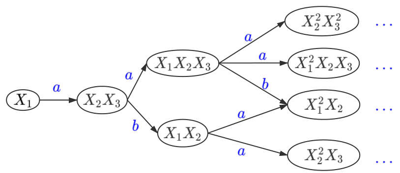
Given a BPP, where symbol set and rule set consists of rules , , . Start from the BPP expression , the state transition is shown in Figure 1.
2.2 CTL
Computation Tree Logic (CTL) is a branching-time logic, which means the model of time is a tree-like structure, in the future there’re different paths. A CTL formula uses logical operators and temporal operators, the logical operators are the usual ones: ; the temporal operators include quantifiers over paths which means all paths and exist one path and path-specific quantifiers:. means ’Next’, means ’Globally’, means ’Until’ and means ’Finally’. One minimal set of operators is: {true, }. In this paper we focus on the fragment of CTL called with the following syntax
| (2) |
where . is an atomic fomrula of the form as , where , .
Example 2
The the duality AF operator can be defined as: . The formula denotes that ” If the sum of and in a state is at least 3, then this state exists a subsequent state passing action whose number of the process is greater than or equal to 1” will be satisfied at some point in the future.
If a formula contains no EF operator we call it an EG-formula; if it contains no EG operator we call it an EF-formula. In terms of the complexity of model checking problem for EG-formulas(i.e. liveness problem) on BPPs, Esparza [12] proved the following theorem:
Theorem 2.1
The model checking problem for EG-formulas on BPPs is undecidable.
EF-formulas can define the reachability properties [3]. For the complexity of model checking EF (i.e. reachability problem) on BPPs, Esparza [11] proved the following theorem:
Theorem 2.2
The model checking problem for EF-formulas on BPPs is NP-complete.
2.3 Actor Communicating System
Actor Communicating System (ACS) is a sound model for asynchronously communicating programs proposed by Osualdo [9]. ACS contains behaviors of creating processes, sending messages and receiving messages. The formal definition of ACS is defined as follows.
Definition 2
An ACS is a 4-tuple , where is a finite set of control states, is a finite set of process states, is a finite set of messages and is a finite set of transition rules. For , can be written as , where and , p!m (send message to process ), (receive message from process )}.
We define that denotes , and that denotes the reflexive transitive closure of . Semantically, ACS does not remember the order of messages in a mailbox, instead it uses a counter abstraction on the mailbox, recording the number of messages in the mailbox. ACS also use a second counter on the control state of each process class to count the process in the current control state. So we further use a VAS (short for Vector Addition System [18]) to express the semantics of ACS intuitively.
Thus The semantics of ACS can be defined as a transition system generated by VAS , where the set of places . We denote the vector set as a place of , where vector contains counters of all states and vector contains counters of messages in mailbox. Finally, we introduce two self-defined symbols: denotes the number of state and symbol denotes the count of in ’s mailbox.
3 Model Checking EF-formulas and EG-formulas
This section provides our reduction of model checking EF-formulas and EG-formulas on BPP. First, we reduce the model checking problem of EF-formula to the satisfiability of existential Presburger formulas [31]. Second, we reduce the bounded model checking problem of EG-formula to the satisfiability of linear integer arithmetic (LIA) in steps.
3.1 EF-formulas: Construction of Existential Presburger Formula
The existing idea of NP-complete model checking is to reduce the problem to smaller computing objects and solve it by efficient SMT solvers. Verma et al. proved that the Parikh image of context-free grammar could be reduced to the satisfiability of existential Presburger formula [34]. However, there is a problem with this reduction, which makes the formula constructed too few constraints. Barner proposed a new version and corrected the problem [2]. We implements the reduction method equivalent to Barner’s version logic proposed by Hague [16].
Given a BPP expression and an initial BPP expression . We assume that contains only one symbol, and let . We introduce variables:
- •
, introduce representing the number of times that process appears;
- •
, introduce representing the number of times that rule is used;
- •
According to the transition rule, define a spanning tree whose nodes are process symbols and introduce representing the distance from to .
Now we can construct the existential Presburger formula, which contains two parts of constraints. The first part mainly expresses that the number of times a transition rule is used must be consistent with the number of symbols appear in the BPP expression. For example, if is the only rule that generates (i.e. ), then . As described above, the first part consists of following constraints:
- •
For , introduce constraint:
- •
For , introduce constraint:
- •
Let be rules whose left symbol is , note that symbol represents the number of in , introduce constraint:
(3)
For any reachable state , the second part rely on to describe the precondition that rules that generate must be used at least once.
- •
For , introduce constraint:
- •
Let be rules whose right symbol is , be left symbols of corresponding rules, introduce constraint:
(4)
3.2 Bounded EG-formulas: Linear Integer Arithmetic
According to Theorem 2.1, model checking EG on BPP is undecidable so we cannot efficiently perform model checking liveness on BPP under standard semantics. A labelled transition system generated by a BPP and an initial BPP expression may have infinitely long but non-cyclic paths, resulting in an increasing number of process symbols of BPP states. In reality, however, most programs can terminate within a finite number of steps, so the number of processes does not tend to be infinite and the transition of a process tend to stop within a certain number of steps. Based on these observations, we present an approach for bounded model checking of EG-formulas on BPP, which is combined with ideas from our previous work [8, 33, 35]. Our approach contain three parts: (i) Proposing the -step bounded semantics of EG: . (ii) Constructing the corresponding linear integer arithmetic (LIA) for the given BPP and EG-formulas. (iii) Using our tool to solve the satisfiability of linear integer arithmetic.
K-step Bounded Semantics.
We give the -step bounded semantics for EG-formulas, limits a BPP state to satisfying properties within steps.
Definition 3
Let be a BPP expression, be an EG-formula, , then the -step bounded semantics is inductively defined as:
- •
iff ,
- •
iff is false,
- •
iff and ,
- •
iff and there exists a state such that and ,
- •
iff there exists a path such that and .
Note that for , since the satisfication of needs at least 1 transition so the number of steps has a lower bound 1.
Algorithm for LIA Construction.
Linear integer arithmetic is a first-order theory and the syntax of linear integer arithmetic is : , where .
According to -step bounded semantics of EG-formulas given above, we can construct the corresponding LIA. we first define some basic constraints to represent BPP’s behavior and then give an algorithm to construct LIA.
Constraints.
Firstly, we introduce some basic symbols and mappings. Similar with the definition in Petri nets, for each rule , define as symbols on the left, as BPP expressions on the right and as the action. For example, if , then and .
Define mapping like Parikh mapping , where each element represents the number of symbols - 1. For example, . Given , n-dimensional vector and , define as:
| (5) |
Note that reflects the change of the number of process symbols after arrives at through transition rule . Based on , we now give the definition of transition constraints (i.e. ) that restricts each component of a legal BPP expression to be non-negative:
| (6) |
is necessary for the transition to be triggered, guaranteeing the requirement of BPP that occurrences of each process symbol in BPP expression cannot be negative. We define path constraints as:
| (7) |
can use the rule to arrive , which corresponds to .
The Algorithm generating corresponding LIA is presented in Algorithm 1. The algorithm is a recursive function, which recurses according to the structure of EG-formula . If is an atomic formula, the corresponding constraints in the semantic definition are generated. If the outermost layer of is a logical proposition operator, it is constructed according to the semantics of negation and conjunction. For or , the corresponding LIA formula is generated through transition and path constraints under the bounded semantics. Finally, it returns a closed LIA formula.
;
;
end case 12
We state that Algorithm 1 is sound: If all components of the input vector are greater than 0 and the generated formula is satisfied, then any variable in are non-negative, (i.e. ). As decribed above, we give the following lemma and theorem:
Lemma 1
Given , two -dimensional vectors: and . If , , and , then .
Proof
According to the definition of and mapping , for any , we can get that . At the same time, is satisfied. We can discuss the following two cases:
- •
If does not equal to , then ;
- •
If equals to , then .
This concludes the proof of lemma 1. ∎
Using the Lemma 1, we can now prove the following theorem:
Theorem 3.1
Given an EG-formula , a -dimensional vector and non-negative integer . Suppose is or . If and , , then any additional variables produced in the construction of LIA through , are nonnegative (i.e. ).
Proof
According to the type of , we discuss the following two cases:
- •
Suppose that is .
During the construction of , new variables are , and is satisfied. Then from the definition of
, there exists an , s.t. , and . So from Lemma 1, . - •
Suppose that is .
During the construction of , new variables are . We prove this theorem by structural induction on , the step size.
Basis: For , . Therefore new variables are non-negative.
Induction step: Assume that and the theorem is true for steps, i.e. are non-negative. According to , there exists , s.t. and is satisfied. So from Lemma 1, are non-negative.
This concludes the proof of Theorem 3.1. ∎
According to Algorithm 1, it will produce new variables only when meet operators and EG operators. So according to Theorem 3.1, as long as the input is a legal BPP state (i.e. each component of the vector is non-negative), the coding based on Algorithm 1 will not produce an illegal BPP state. Then the reliability and soundness theorem of Algorithm 1 is stated as follows:
Theorem 3.2
Given an EG-formula , a n-dimensional vector , and a natural number , Algorithm 1 is correct:
- •
Termination: The algorithm will terminate after a finite number of steps.
- •
Reliability: If , then is satisfied.
- •
Soundness: If is satisfied, then .
Proof
Since Algorithm 1 constructs LIA formula recursively over the structure of EG-formula , it can be concluded that Algorithm 1 terminates. For reliability and soundness, we prove their correctness by structural induction on :
- •
Suppose that is an atomic proposition, i.e. , then from the definition , reliability and soundness are satisfied.
- •
Suppose that .
For reliability, assume that is unsatisfied, then according to Algorithm 1, is unsatisfied, so is correct. By induction hypothesis, is satisfied so is unsatisfied.
For soundness, whereas, assume that is correct, then according to Algorithm 1, is unsatisfied. By induction hypothesis, is unsatisfied so is satisfied.
- •
Suppose that .
For reliability, assume that is unsatisfied, then according to Algorithm 1, is unsatisfied, so is unsatisfied or is unsatisfied. By induction hypothesis, or is unsatisfied so is unsatisfied.
For soundness, assume that is correct, then according to Algorithm 1, is unsatisfied and is unsatisfied. By induction hypothesis, and are unsatisfied so is satisfied.
- •
Suppose that .
For reliability, assume that is unsatisfied, then or, for any , if , then . If , obviously . For the latter, assume that is correct for any , then is correct, therefore is unsatisfied. By induction hypothesis,
is unsatisfied, so is satisfied. In conclusion, is unsatisfied.For soundness, assume that is correct, then and there exists , s.t. , so is unsatisfied. By induction hypothesis,
is unsatisfied, so is satisfied. In conclusion, is satisfied. - •
Suppose that . Let in the Algorithm 1.
For reliability, assume that is unsatisfied, then for any , if formula is satisfied, then
. So there exists ,
s.t. is satisfied, so we find unsatisfied. By induction hypothesis, is unsatisfied, so is satisfied, i.e. is unsatisfied.For soundness, assume that is correct, then there exists , s.t. . So for any , is unsatisfied. By induction hypothesis, is unsatisfied, i.e. is satisfied. In conclusion, is satisfied.
This concludes the proof of Theorem 3.2. ∎
4 ACS2BPP: Reduction from ACS to BPP
In this section, we introduce the ACS2BPP module of BPPChecker. We give Actor Communicating System (ACS) the over-approximation BPP-based semantics to reduce ACS to BPP. With the support of the Erlang verifier Soter and ACS2BPP module, we can easily transfer Erlang programs to ACS and then verify EF-formulas defined safety properties on ACS.
4.1 BPP-based Semantics of ACS
Considering the case when the rule of ACS is used, we can observe that two symbols will decrease at the same time: (i) The number of state will decrease as it transfers to ; (ii) The side-effect of will consume a message from its mailbox. In this case, the value of two different symbols should be decreased at the same time, whereas the rule of BPP only allows one symbol to appear on the left side.
So we adapt two rules of ACS to BPP so that we can use BPP to simulate and verify ACS [32]. The modification is to add two labels and to each message, respectively recording the history of the message arriving and leaving the mailbox. The mapping from mailbox to message is now replaced with , then the BPP semantics of ACS is defined as follows:
Given an ACS , we construct BPP, where . For , according to the type of , we define as :
- •
, add a rule ;
- •
, add a rule ;
- •
, add a rule ;
- •
, add a rule
4.2 Place Convert Function
We also give an algorithm called place convert function for transforming places from original semantics to BPP-based semantics.
Given an ACS , where , input a place under the original semantics to place convert function will output a new place satisfying transformation as follows:
- •
, ;
- •
, ;
- •
,.
Under the new semantics, the state counter remains unchanged, while the message counter change. For process and message , the number of in equals to the number of in in the original semantics and the initial count in is 0. When consumes message , the original rule reduces in , while the new rule increases in p.
We state that the BPP-based semantics of ACS is an over-approximation of ACS, which means it contains more behaviors than the original semantics. The following Theorem 4.1 proves that for any reachable place under the original semantics, there exists an reachable place , whose number of states is the same as that of and the difference between and in equals to the number of in .
Theorem 4.1
Given an ACS , where , where , and given a place under the original semantics, if there exists that satisfies:
- •
;
- •
, where denotes messages of ;
- •
,
then there exists a place under the BPP-based semantics such that:
- •
;
- •
, where denotes messages of ;
- •
;
- •
, where is the output of place convert function with the input .
Proof
We prove the correctness of Theorem 4.1 by structural induction:
Basis step: is , then the output is the place of new semantics.
Induction step: Without loss of generality, let , and , then we discuss the cases of as below:
- •
op=nop.
According to the rule of ACS semantics and is satisfied. By induction hypothesis, there exists the place under the new semantics, s.t. , and at the same time . So . Therefore we can get , in which and . Beyond that has no other side-effect, so the place is eligible.
- •
.
According to the rule of ACS semantics and is satisfied. By induction hypothesis, there exists the place under the new semantics, s.t. , and at the same time . Therefore we can get , in which , and . Beyond that is consistent with . So is eligible.
- •
.
According to the rule of ACS semantics satisfies that . By induction hypothesis, there exists the place under the new semantics, s.t. , and at the same time , . We can get , in which , and . So,
Beyond that other elements are consistent, so and is eligible.
- •
.
According to the rule of ACS semantics satisfies that . By induction hypothesis, there exists the place under the new semantics, s.t. , and at the same time , . We can get , in which , and . So,
Beyond that other elements are consistent, so and is eligible.
This concludes the proof of Theorem 4.1. ∎
So when the reachability (EF-formulas) of BPP is unsatisfied, the corresponding state in ACS is also unreachable.
Based on above techniques, our tool can verify safety properties of ACS and even Erlang programs more efficiently because we reduce the complexity from EXPSPACE-complete to NP-complete [28, 11]. More specifically, safety properties include the unreachability of errors, boundedness of mailbox in system etc. Here we omit formal descriptions of safety properties due to space considerations and a case study is given in the following section to help understand.
4.3 Case Study
We give a case study of how BPP-based model checking of ACS combining techniques proposed above works.
Given an ACS , where , , and . We assume that the initial place under original semantics satisfies: and .
Figure 2 shows the ACS generated by our BPP-based semantics. Each node represents a place and each directed edge represents a transition rule. The superscripted item like means the mapping of place satisfies .

It is obvious that at any time the number of and should not be larger than one, and process contains a maximum of one message. So we can define the above two reachability properties of in the form of CTL formulas: (i) Neither nor can be satisfied. (ii) The formula can not be satisfied.
Given the information of BPP model and specification of properties, we can verify the safety properties of ACS by model checking the CTL on BPP and get the result.
Over-approximation Semantics Descriptions.
We also give an example here to show the over-approximation of our BPP-based semantics against original semantics. Consider a ACS , where consists of two rules: , . Assume that in the initial place mailbox of is empty. Intuitively, the original semantics require that a message can be consumed only when at least one message is in the mailbox. So first uses to pattern-match and then consume using . The BPP-based semantics, however, allow to consume without containing the , i.e., the initial place generated by place convert function can use both and .
5 Tool Implementation
In this section, we provide more details of design and implementation of BPPChecker. The overall architecture of BPPChecker is presented in Figure 3.
Overview of structure.
BPPChecker uses the Python3 interface of SMT solver Z3(v4.8.5) as a library for solving linear integer arithmetic. Through input files, users provide information on BPP and CTL formulas. Through instructions, users can specify the step size of bounded EG model checking and whether to output additional information besides the solved result. BPPChecker is mainly divided into three modules: (i) syntax parser; (ii) BPP and formula model; (iii) a model checker which implements the algorithms in Section 3.

Input and syntax parser (run.py and parser.py).
The tool first checks whether a given input file conforms to the definition of BPP and CTL grammar. We ask the user to provide information about the BPP model and the initial BPP expression. For bounded EG verification, the step size should be given through instruction as a parameter. The detailed syntax of input is shown in Figure 4. If the input is illegal, the tool reports an error and stops execution. Otherwise, the syntax parser will construct the BPP and generate the corresponding constraints to continue. Figure 5 and Figure 5 show an example of input to BPPChecker.
PROBLEM BPP ”formula” FORMULA BPP ”initial” SYMBOLS ”rules” RULES SYMBOLS VAR — SYMBOLS ”,” SYMBOLS RULES RULE — RULES RULES RULE VAR ”” SYMBOLS — VAR ”” LABEL ”” SYMBOLS FORMULA UNARY ”(” FORMULA ”)” — BINARY ”(” FORMULA ”,” FORMULA ”)” — NEXT ”(” LABEL ”,” FORMULA ”)” QUERY ACC COMPARE NUMBER ACC MULT — ACC CONNECT ACC MULT VAR — VAR ”” NUMBER CONNECT [] COMPARE ”==” — ”!=” — ”¿=” — ”¡=” — ”¿” — ”¡” UNARY ”Neg” — ”EG” — ”AF” — ”EF” BINARY ”Conj” — ”Disj” — ”Imp” NEXT ”EX” — ”AX” VAR [a-zA-Z][a-zA-Z0-9]⋆ LABEL [a-zA-Z][a-zA-Z0-9]⋆ NUMBER [1-9][0-9]⋆
ACS2BPP converter (ACS2BPP.cpp).
In the module of ACS2BPP, we implement the algorithm described in Section 4 that converts an Actor Communicating System to BPP. With the support of ACS2BPP, given an ACS model, we can firstly input it to ACS2BPP and then verify safety properties of an ACS through BPPChecker.
Model checker (bpp.py, blchecker.py, rchecker.py).
Output.
The output contains solved result and time. Optionally, users can choose to output set of constraints constructed from statistics provided by Z3 solver. If the input problem can be satisfied, the model is returned (i.e. a set of assignment for each variable). Otherwise, constraints that caused the contradiction are returned. Figure 5 shows a satisfied model of Figure 5.
(x_S, 0) (x_X, 1) (x_Y, 1) (y_1, 1) (y_2, 1) (z_S, 0) (z_X, 1) (z_Y, 2)
6 Evaluation
6.1 Bounded Model Checking of EG-formula
In terms of BPP model, we use the BPP shown in Example 1 as the experimental model. Based on this BPP, we perform the model checking against the following EG-formulas:
| (8) |
Bounded model checking is conducted when step is respectively set to 5, 10, 20 and 50. Experimental results are shown in Table 1, in which we show the time(s) spent to verify each case.
| 5 | 10 | 20 | 50 | |
|---|---|---|---|---|
| 0.024 | 0.047 | 0.072 | 0.253 | |
| 0.033 | 0.058 | 0.114 | 0.245 | |
| 0.092 | 0.269 | 0.981 | 6.259 |
From the experimental results, we know that the time spent of BPPChecker increases as step increases. The nested depth of formula is longer than that of and , however, the time of solving is only slightly longer than that of solving , while the time of solving is much longer than that of solving the other two formulas. This situation is especially obvious when the factor() is large. This is because the number of variables is the main factor that limits the tool’s speed. For EG operator, as defined in Algorithm 1, constructing LIA formulas needs variables, where is the number of process symbols of BPP. Formula is in fact logically equivalent to formula . So the number of variables in the LIA formula generated by is . As a result, when gets larger, the solver will spend longer time.
For liveness (EG-formulas) properties, existing verifiers based on Petri net are oriented to traditional Petri nets, whose standard benchmarks are no longer applicable to BPP model. In order to evaluate different factors, we generate test cases randomly and run experiments on BPP with different sizes and various step sizes. Since the size of BPP is mainly reflected in the number of transition rules, we model check BPPs with transition rules of 10,20 and 30. For EG-formula, we still choose , and above.
| 10 | 0.330 | 0.348 | 1.293 | |
| 20 | 1.153 | 1.336 | 3.693 | |
| 30 | 2.097 | 2.376 | 7.920 | |
| 10 | 0.636 | 0.672 | 3.785 | |
| 20 | 2.231 | 2.587 | 13.889 | |
| 30 | 4.262 | 4.706 | 28.558 | |
| 10 | 0.918 | 1.050 | 8.075 | |
| 20 | 3.348 | 3.809 | 26.884 | |
| 30 | 7.249 | 8.353 | 56.810 |
Table 2 depicts experimental results in seconds(s). The time spent increases as the number of rules and increases. The size of rule set affects the size of the disjunctive formula in the transition constraints and path constraints because we need to search the rules in BPP rule set to validate transitions and paths. The step size mainly determines the size of conjunction formula in the path constraints of LIA formula corresponding to the outermost formula whose temporal operator is EG, i.e. the number of sub-constraints. Last but not least, also has an impact on the number of variables introduced.
6.2 Model Checking on ACS
To evaluate the model checking on our BPP-based ACS semantics, we do experiments on ACSs generated from real Erlang asynchronously communicating programs. The benchmark we use are offered by Osualdo’s work named Soter [9, 17], an automatic and efficient ACS-based model checking tool for Erlang. We experimentally compare our BPPChecker with Soter’s backend BFC, where BFC verifies reachabillity (i.e. EF-formula) on ACS of Erlang programs and BPPChecker verifies BPPs generated by our module. Table 3 shows that BPPChecker takes less time than the BFC in almost all test cases. Moreover, rules constructed by BPP-based semantics of ACS are also less. As a result, BPPChecker performs better in both time and number of rules.
The above experiments on real Erlang programs also show that BPPChecker has universality in real asynchronous communicating programs verfication: It supports higher-order functions such as Erlang programs, process creation, behaviors of the asynchronous messaging, verfication of error reachability problem and even mutual exclusivity (an important property of asynchronous and concurrent programs). Besides, our approach can be flexibly applied to verify number of messages in a specific mailbox, validating the effectiveness of operation order, security setting, etc.
| Test Case | BFC | BPPChecker | ||
|---|---|---|---|---|
| Number of Rules | Time(s) | Number of Rules | Time(s) | |
| pipe | 14 | 0.106 | 9 | 0.025 |
| ring | 40 | 0.268 | 28 | 0.106 |
| state_factory | 34 | 0.736 | 22 | 0.074 |
| reslock | 52 | 0.821 | 38 | 0.228 |
| reslockbeh | 62 | 0.856 | 46 | 0.268 |
| parikh | 31 | 0.070 | 20 | 0.097 |
7 Related Work
Verification of concurrent programs mainly relies on approximation or abstraction to limit the program model. Most verfication of concurrent programs are done on Petri nets or its extentions due to its high complexity [15, 20]. Sen and Viswanathan [30] proposed a multi-set pushdown system with empty stack restriction. Emmi [10] proposed an event-driven asynchronous program model, which reduced the coverage of v-PN and concluded that the state reachability of multi-set pushdown system was decidable. Kochems [21, 27] proposed a looser K-shaped limitation to limit the number of stack symbols for receiving operations on the stack of any process and proposed a theoretical model Nets with Nested Colored Tokens (NNCT) based on Petri Nets. Osualdo proposed Actor Communicating System with finite-state processes and implemented Soter, a verifier for Erlang programs. Despite the wide use of Petri nets [26], the time complexity of many branching-time properties on it is very high. Reachability problem on Petri nets has an ACKERMANN upper bound [22] and a Tower-hard lower bound [6]. Czerwińsk further improved the lower bound and proved that without restriction on dimension, the problem needs a tower of exponentials of time or space, of height exponential in input size [7]. As for coverability and boundedness, their complexity is EXPSPACE-complete [28, 11]. For NNCT, coverability is TOWER-complete, while boundedness and termination are TOWER-hard [20]. So existing automatic tools such as BFC [17], IIC [19] and Petrinizer [13] cannot perform well for large-scale programs, and the tools are difficult to be complete and efficient.
Different from general Petri nets, many properties on BPP have low complexity. Esparza proved the following conclusions [12, 24]: (i) Model checking reachability on Petri nets is undecidable, but for BPP, even if finite-state BPP, the problem is PSPACE-hard; (ii) Given fixed formulas with fixed length, model checking reachability on BPP is complete, where is the nested depth of modal operator . On the basis of this conclusion, Mayr proved that model checking EF on BPP is actually PSPACE-complete [23].
8 Conclusion
Basic Parallel Process (BPP), as a subclass of Petri nets, can be used to verify concurrent programs with lower complexity. We implement BPPChecker, the first SMT-based model checker for verifying a subclass of CTL (CTL) on BPP. For EF-formulas model checking, we reduce it to the satisfiability problem of existential Presburger formula. For EG-formulas model checking, we provide a -step bounded semantics and reduce it to the satisfiability problem of linear integer arithmetic. The linear integer arithmetic formulas are handled by SMT solver Z3. We give Actor Communicating System (ACS) the over-approximation BPP-based semantics and evaluate BPPChecker on ACSs generated from real Erlang programs. Experimental results show that BPPChecker performs more efficiently than the existing tools for a series of property verification problems of real Erlang programs. In the future, we plan to enhance our tool by implementing an Erlang-to-BPP converter and focus on more pracitcal problems like dynamic updating through abstract interpretation to CTL formulas on BPP.
References
- [1] Atig, M.F., Bouajjani, A., Qadeer, S.: Context-bounded analysis for concurrent programs with dynamic creation of threads. In: International Conference on Tools and Algorithms for the Construction and Analysis of Systems. pp. 107–123. Springer (2009)
- [2] Barner, S., Seidl, A.P.D.H.: H3 mit gleichheitstheorien. Ph.D. thesis, Diploma thesis, TUM (2006)
- [3] Bérard, B., Bidoit, M., Finkel, A., Laroussinie, F., Petit, A., Petrucci, L., Schnoebelen, P., Mckenzie, P.: Reachability properties. In: Systems and Software Verification, pp. 79–81. Springer (2001)
- [4] Carlsson, R.: An introduction to core erlang. In: Proceedings of the PLI’01 Erlang Workshop. Citeseer (2001)
- [5] Christensen, S.: Decidability and decomposition in process algebras (1993)
- [6] Czerwiński, W., Lasota, S., Lazić, R., Leroux, J., Mazowiecki, F.: The reachability problem for petri nets is not elementary. Journal of the ACM (JACM) 68(1), 1–28 (2020)
- [7] Czerwiński, W., Lasota, S., Orlikowski, Ł.: Improved lower bounds for reachability in vector addition systems. In: 48th International Colloquium on Automata, Languages, and Programming (ICALP 2021). Schloss Dagstuhl-Leibniz-Zentrum für Informatik (2021)
- [8] Ding RJ, L.G.: Efficient implementation of coverability verification on communication-free petri net. Journal of Software 30(7) (2019)
- [9] D’Osualdo, E., Kochems, J., Ong, C.H.L.: Automatic verification of erlang-style concurrency. In: International Static Analysis Symposium. pp. 454–476. Springer (2013)
- [10] Emmi, M., Ganty, P., Majumdar, R., Rosa-Velardo, F.: Analysis of asynchronous programs with event-based synchronization. In: European Symposium on Programming Languages and Systems. pp. 535–559. Springer (2015)
- [11] Esparza, J.: Decidability and complexity of petri net problems—an introduction. In: Advanced Course on Petri Nets. pp. 374–428. Springer (1996). https://doi.org/10.1007/3-540-65306-6_20
- [12] Esparza, J.: Decidability of model checking for infinite-state concurrent systems. Acta Informatica 34(2), 85–107 (1997). https://doi.org/10.1007/s002360050074
- [13] Esparza, J., Ledesma-Garza, R., Majumdar, R., Meyer, P., Niksic, F.: An smt-based approach to coverability analysis. In: International Conference on Computer Aided Verification. pp. 603–619. Springer (2014)
- [14] Fu, H.: Model checking egf on basic parallel processes. In: Bultan, T., Hsiung, P.A. (eds.) Automated Technology for Verification and Analysis. pp. 120–134. Springer Berlin Heidelberg, Berlin, Heidelberg (2011). https://doi.org/10.1007/978-3-642-24372-1_10
- [15] Ganty, P., Majumdar, R., Rybalchenko, A.: Verifying liveness for asynchronous programs. In: Proceedings of the 36th annual ACM SIGPLAN-SIGACT symposium on Principles of programming languages. pp. 102–113 (2009)
- [16] Hague, M., Lin, A.W.: Synchronisation-and reversal-bounded analysis of multithreaded programs with counters. In: International Conference on Computer Aided Verification. pp. 260–276. Springer (2012)
- [17] Kaiser, A., Kroening, D., Wahl, T.: Efficient coverability analysis by proof minimization. In: International Conference on Concurrency Theory. pp. 500–515. Springer (2012)
- [18] Karp, R.M., Miller, R.E.: Parallel program schemata. Journal of Computer and system Sciences 3(2), 147–195 (1969)
- [19] Kloos, J., Majumdar, R., Niksic, F., Piskac, R.: Incremental, inductive coverability. In: International Conference on Computer Aided Verification. pp. 158–173. Springer (2013)
- [20] Kochems, J.: Verification of asynchronous concurrency and the shaped stack constraint. Ph.D. thesis, Oxford University, UK (2014)
- [21] Kochems, J., Ong, C.H.L.: Safety verification of asynchronous pushdown systems with shaped stacks. In: International Conference on Concurrency Theory. pp. 288–302. Springer (2013)
- [22] Leroux, J., Schmitz, S.: Reachability in vector addition systems is primitive-recursive in fixed dimension. In: 2019 34th Annual ACM/IEEE Symposium on Logic in Computer Science (LICS). pp. 1–13. IEEE (2019)
- [23] Mayr, R.: Weak bisimulation and model checking for basic parallel processes. In: International Conference on Foundations of Software Technology and Theoretical Computer Science. pp. 88–99. Springer (1996)
- [24] Minsky, M.L.: Computation. Prentice-Hall Englewood Cliffs (1967)
- [25] Nieuwenhuis, R., Oliveras, A., Tinelli, C.: Solving sat and sat modulo theories: From an abstract davis–putnam–logemann–loveland procedure to dpll (t). Journal of the ACM (JACM) 53(6), 937–977 (2006)
- [26] Petri, C.A.: Communication with automata (1966)
- [27] Qadeer, S., Rehof, J.: Context-bounded model checking of concurrent software. In: International conference on tools and algorithms for the construction and analysis of systems. pp. 93–107. Springer (2005)
- [28] Rackoff, C.: The covering and boundedness problems for vector addition systems. Theoretical Computer Science 6(2), 223–231 (1978)
- [29] Ramalingam, G.: Context-sensitive synchronization-sensitive analysis is undecidable. ACM Transactions on Programming languages and Systems (TOPLAS) 22(2), 416–430 (2000)
- [30] Sen, K., Viswanathan, M.: Model checking multithreaded programs with asynchronous atomic methods. In: International Conference on Computer Aided Verification. pp. 300–314. Springer (2006)
- [31] Stansifer, R.: Presburger’s article on integer arithmetic: Remarks and translation. Tech. rep., Cornell University (1984)
- [32] Tan, J.: Research on verification of asynchronously communicating program based on Basic Parallel Processes. Master’s thesis, Shanghai Jiao Tong University (2020)
- [33] Tan JH, L.G.: Bounded model checking liveness on basic parallel processes(in chinese). Journal of Software 31(8), 2388–2403 (2020)
- [34] Verma, K.N., Seidl, H., Schwentick, T.: On the complexity of equational horn clauses. In: International Conference on Automated Deduction. pp. 337–352. Springer (2005)
- [35] Yang QZ, L.G.: Model on asynchronous communication program verification based on communicating petri nets(in chinese). Ruan Jian Xue Bao/Journal of Software 4 (2017)