Arjun: An Efficient Independent Support Computation Technique and its Applications to Counting and Sampling Thanks: The tool is available open-source at https://github.com/meelgroup/arjun Affiliation: National University of Singapore

Given a Boolean formula $\varphi$ and a projection set $\mathcal{P}\subseteq X$, the problem of projected model counting seeks to compute the number of solutions of the formula $\exists Y\varphi$ where $Y=X\setminus\mathcal{P}$; alternatively, the solutions of the formula $\exists Y\varphi$ can be viewed as solutions of the formula projected on $\mathcal{P}$. Observe that projected model counting is a strict generalization of the classical problem of propositional model counting which focuses on the case when $\mathcal{P}=X$. Similarly, the problem of projected sampling seeks to uniformly sample solutions of $\exists Y\varphi$.

Projected counting and sampling are fundamental problems in computer science with a wide variety of applications ranging from network reliability [7], neural network verification [1], computational biology [23], and software and hardware testing [18]. For example, given a neural network $\mathcal{N}$ and a property $\psi$, the problem of estimating how often the network satisfies the property $\psi$ reduces to projected counting [1].

From a theoretical viewpoint, projected counting is #NP-complete; it is worth remarking that the problem of propositional model counting is #P-complete [28], and it is known that #P $\subseteq$ #NP. The hardness of #P (and #NP) motivated efforts towards approximation methods with $(\varepsilon,\delta)$-guarantees. The state of the art approximate techniques for counting and sampling are hashing-based [3, 4, 5, 27, 26], seeking to combine the power of universal hash functions with advances in SAT solving.

The core idea of hashing-based counting techniques is to employ pairwise independent hash functions, also known as strongly universal hash functions, to partition the solution space into roughly equal small cells of solutions and then pick a cell randomly. The number of solutions in a cell can then be determined exactly by enumerating the solutions in the cell one by one, in case the cell is small. The number of solutions of the formula is then estimated as the number of solutions of a randomly chosen small cell multiplied by the number of cells. In case of sampling, we enumerate the solutions in the cell and chose one of the solutions uniformly at random.

To achieve estimates with rigorous $(\varepsilon,\delta)$-guarantees (formally defined in Section 2), we use 3-wise independent hash functions¹¹ 1 The hashing-based counting technique only require 2-wise independent hash functions but the current state of the art hashing-based sampling techniques rely on 3-wise independent hash functions. The current state of the art techniques rely on XOR-based 3-wise independent hash functions. A randomly picked hash function $h:\{0,1\}^{n}\mapsto\{0,1\}^{m}$ is explicitly represented as a conjunction of $m$ randomly chosen XOR constraints, where each constraint is constructed by picking every variable with probability $\frac{1}{2}$. Therefore, the expected size of each XOR is $\frac{n}{2}$ where $n=|\mathcal{P}|$. Accordingly, the SAT solver is invoked to find solutions of a formula expressed as conjunction of the original formula, $\varphi$, and the XOR constraints.

Runtime performance of hashing-based counting and sampling techniques is primarily determined by the time taken by the SAT solver as over 99% of the time is spent inside SAT calls. Accordingly, the past decade has witnessed a sustained effort in designing sparse XOR-based hash functions [10, 9, 5, 16]. An important advance in this direction was achieved by Chakraborty et al. [5], who proposed the notion of independent support and observed that one can construct XORs only over the given independent support. It is worth remarking that Chakraborty et al. had defined the notion of independent support $\mathcal{P}=X$ but one can see that the notion easily generalizes to arbitrary $\mathcal{P}$.

Ivrii et al. [11] showed that the problem of computation of Minimal Independent Support can be reduced to Group Minimal Unsatisfiable Subset (GMUS), and the corresponding tool, $\mathsf{MIS}$, was shown to scale to moderately complex instances. Concurrently, Lagniez et al. [12, 13] published a pre-processing technique, B+E, that combines the assumption-based framework offered by modern CDCL solvers with Padoa’s theorem [20] to identify an independent support. An important conceptual viewpoint put forth by Lagniez et al. was the argument of eschewing the search for minimal independent support and instead focus on efficiently finding an independent support that may not be necessarily minimal.

Our primary contribution is the design of an efficient framework, called $\mathsf{Arjun}$, to identify independent support. $\mathsf{Arjun}$ consists of two phases. The first phase employs a syntactic gate recovery-based strategy while the second phase is based on the tight integration of the standard assumption-based CDCL framework with the invocations needed to execute on Padoa’s Theorem [20].

To demonstrate the efficacy of our approach, we perform a detailed empirical analysis over an extensive set of 1896 benchmarks arising from a diverse set of domains and employed in the analysis of counting and sampling techniques. We first showcase that with a timeout of 5000 seconds, $\mathsf{Arjun}$ can compute independent support for 358 more instances than the state of the art tool, $\mathsf{MIS}$.

We observe that $\mathsf{ApproxMC4}$ augmented with $\mathsf{Arjun}$ can count 1596 benchmarks, achieving an improvement of 387 benchmarks over $\mathsf{ApproxMC4}$. Similarly, we observe that $\mathsf{UniGen3}$ augmented with $\mathsf{Arjun}$ can sample 1354 benchmarks, achieving an improvement of 319 benchmarks within the same time limit of 5000s. Furthermore, we observe a significant improvement in runtime performance as well, in particular, the PAR-2 scores²² 2 PAR-2 scores are used in the SAT competitions to measure performance. Each benchmark contributes a score that is the number of seconds used to finish (e.g. solve, count, sample) it, or in case of a timeout or memory out, twice the timeout in seconds. We then calculate the average score for all benchmarks, giving PAR-2. for $\mathsf{ApproxMC4}$ and $\mathsf{UniGen3}$ augmented with $\mathsf{Arjun}$ are 1707 and 2957 while the PAR-2 scores for $\mathsf{ApproxMC4}$ and $\mathsf{UniGen3}$ are 3800 and 4717, respectively.

Furthermore, $\mathcal{I}\subseteq\mathcal{P}$ is called minimal independent support of $\mathcal{P}$ if there does not exist $\hat{\mathcal{I}}\subset\mathcal{I}$ such that $\hat{\mathcal{I}}$ is an independent support.

Observe that if $\mathcal{I}$ is an independent support of $\mathcal{P}$, then we have $|sol({\varphi})_{\downarrow\mathcal{I}}|=|sol({\varphi})_{\downarrow\mathcal{P}}|$. The notion of independent support is related to the classical notion of definability. To this end, we first present the following two equivalent notions of definability.

Since implicit and explicit definability are equivalent, we can omit referencing them and simply make statements such as: $x$ is defined by $\mathcal{I}$ for the formula $\varphi$. Furthermore, the following remark follows from the notion of Independent support.

The problem of propositional model counting is to compute $|sol({\varphi})|$ for a given CNF formula $\varphi$. A probably approximately correct (or $\mathsf{PAC}$) counter is a probabilistic algorithm ${\mathsf{ApproxCount}}(\cdot,\cdot,\cdot)$ that takes as inputs a formula $\varphi$, a tolerance $\varepsilon>0$, and a confidence $1-\delta\in(0,1]$, and returns a count $c$ with $(\varepsilon,\delta)$-guarantees, i.e., $\mathsf{Pr}\Big[\frac{|sol({\varphi})|}{(1+\varepsilon)}\leq c\leq(1+\varepsilon)|sol({\varphi})|\Big]\geq 1-\delta$. Projected model counting is defined analogously using $sol({\varphi})_{\downarrow\mathcal{P}}$ instead of $sol({\varphi})$, for a given projection set³³ 3 Projection set has been referred to as sampling set in prior work [5, 17] $\mathcal{P}\subseteq X$.

A uniform sampler outputs a solution $y\in sol({\varphi})$ such that $\mathsf{Pr}[y\text{ is output}]=\frac{1}{|sol({\varphi})|}$. An almost-uniform sampler relaxes the guarantee of uniformity and in particular, ensures that $\frac{1}{(1+\varepsilon)|sol({\varphi})|}\leq\mathsf{Pr}[y\text{ is output}]\leq\frac{1+\varepsilon}{|sol({\varphi})|}$.

Given a formula $\varphi$ and a projection set $\mathcal{P}$, we focus on finding the subset of variables $\mathcal{I}\subseteq\mathcal{P}$ along with the set of definitions $\Phi$ such that for every $x\in\mathcal{I}$, there is a corresponding definition $\phi\in\Phi$ such that $\phi$ is defined over $\mathcal{I}$. A possible method for the same can be to rely on Slivovky’s observation of extractions of definitions from the resolution proofs but such a technique is computationally expensive given the requirement of SAT calls.

We observe that syntax-based gate identification techniques such as [19] can be employed on the CNF to efficiently recover an incomplete set of definitions. Given the set of such definitions, we can extract $\mathcal{I}$ and $\Phi$ with the desired properties. Our explicit definability-based identification phase consists of three steps:

We now discuss Step 1 and Step 3 in more detail. First of all, we focus on two set of operators: AND $(\wedge)$ and XOR $(\oplus)$. We detect AND gates of length two while we detect XOR gates of length up to five, both over literals rather than variables. Our advanced AND gates detection works up to length two only, since 2-long AND gates account for the overwhelming set of AND gates present in the benchmarks of interest. Since we focus on variables rather than literals, detection of OR gates is not required, since an OR gate is equivalent to an AND gate on the opposite literals due to De Morgan’s laws [6]. For the algorithm used to efficiently detect AND gates, see Appendix 0.A.1.

In case of XOR gates, we rely on the bloom-filter based XOR recovery algorithm proposed by [27]. We instantiate this recovery algorithm to find XORs of length up to five in order to limit potential explosion of search space. Unlike AND gates, the identification of XOR equation does not put restrictions on the outputs and inputs. In particular, observe that an XOR $\ell_{1}\oplus\ell_{2}\oplus\ell_{3}=1$ can be rewritten in the following ways: (1) $\neg\ell_{1}=\ell_{2}\oplus\ell_{3}$, (2) $\neg\ell_{2}=\ell_{1}\oplus\ell_{3}$, and (3) $\neg\ell_{3}=\ell_{1}\oplus\ell_{2}$. Therefore, given an XOR of length $k$, we extract $k$ definitions.

We now return to Step 3, performing a greedy search to compute $W\cup\mathsf{Root}(G)$ wherein W is a feedback vertex set of $G$. While ideally, we would like $W$ to be a minimal feedback vertex set, we trade off the minimality for runtime performance. The key strategy is to sort the vertices according to the number of edges incident onto them; i.e., we observe that the higher the number of edges incident upon a vertex $u$, the higher likelihood of $u$ to belong to $\mathcal{I}$. We present the pseudocode of the greedy search in Algorithm 2. The algorithm $\mathsf{GreedyIndSearch}$ relies on the array $\mathsf{incidence}$ that is computed for each variable $u$ as the number of clauses containing $u$ or $\neg u$ in $\varphi$.

As noted in Section 2, Lagniez et al. observed that one can iteratively identify independent support. We first extend Lagniez et al.’s proposal to handle projection set and present the resulting pseudocode, called $\mathsf{SimpleSearch}$, in Algorithm 3.

$\mathsf{SimpleSearch}$ takes in a formula $\varphi$ and a projection set $\mathcal{P}$, and returns the independent support $\mathcal{I}$. Without loss of generality, we assume that $\mathcal{P}=\{x_{1},x_{2},\ldots x_{|P|}\}$ (note that simple variable renaming suffices to achieve such a $\mathcal{P}$). The key idea is to construct $\psi$ and perform iterative $\mathsf{solve}$ queries over $\psi$. The standard method is to use assumption-based framework where the solver is required to solve the formula under the set of assumptions expressed as assignment to variables. In $\mathsf{SimpleSearch}$, we maintain two sets: ${\mathsf{unknown}}$, the set of variables that are yet to be classified as dependent or independent and $\mathcal{I}$, the set of variables that we have classified as belonging to the independent support. As will be observed later, we would ideally like to sort the variables in such a way that the variables belonging to the independent support are queried at the very end.

Note that variable $x_{\mathsf{index}}$ can be defined in terms of $\mathsf{unknown}\cup\mathcal{I}$ if and only if $\psi\wedge x_{\mathsf{index}}\wedge\neg y_{\mathsf{index}}$ is UNSAT under the assumption of setting all $z_{i}\in\mathsf{unknown}\cup\mathcal{I}$ to True. Since some SAT calls may be very expensive, instead of invoking the solver to completion, we set a cutoff on the number of conflicts, and therefore, the solver may return SAT, UNSAT, or timeout. To account for timeout, we check, in line 16, whether ret $\not=$ UNSAT instead of checking ret $=$ SAT.

We now seek to understand the key bottleneck for scalability of $\mathsf{SimpleSearch}$: the call to SAT solver on line 15. To this end, we first seek to understand how modern CDCL-based SAT solvers implement the $\mathsf{solve}$ procedure.

Observe that every invocation of $\mathsf{solve}$ on line 15 of $\mathsf{SimpleSearch}$ would require insertion of the set of assumptions of the size $|\mathcal{I}\cup\mathsf{unknown}|$ and the resulting propagations. Since we invoke $\mathsf{solve}$ $|\mathcal{P}|$ times, the underlying solver must deal with $\frac{|\mathcal{P}|^{2}}{2}$ insertions and the corresponding propagations. To put this into perspective, if $|\mathcal{P}|=50000$, then we have over a billion calls to propagate, a relatively expensive operation. At this point, observe that the variable appearing first in ${\mathsf{unknown}}$ is inserted and propagated for all except one $\mathsf{solve}$ call. Therefore, we focus on addressing the performance bottleneck via eliminating redundant work. To this end, the key idea is to pursue a tight integration of $\mathsf{SimpleSearch}$ and the $\mathsf{solve}$ algorithm, combining the two into a single algorithm. For the interested reader, $\mathsf{solve}$, as per the seminal MiniSat paper [8] is explained in Appendix 0.A.2.

The pseudocode for the integrated approach, called $\mathsf{IntegratedImplicit}$, is presented in Algorithm 4. We assume that $\varphi$ is satisfiable, else $\mathcal{I}=\emptyset$ can be returned. Similar to $\mathsf{SimpleSearch}$, we construct the formula $\psi$ based on the input formula $\varphi$. The high-level structure of $\mathsf{IntegratedImplicit}$ is similar to $\mathsf{SimpleSearch}$ with crucial difference arising in the low-level technical details of how to handle the cases when UNSAT, SAT, or the timeout limit is reached.

We now focus on the UNSAT case, i.e., when $x_{\mathsf{index}}$ is shown to be dependent (lines 12– 17). The key observation is that whenever $\varphi$ is satisfiable, then $\psi\wedge\bigwedge_{i=1}^{\mathsf{index}}z_{i}$ is satisfiable. (Observe that $\{z_{i}\}_{i=1}^{\mathsf{index}}$ is conjuncted via $\mathsf{assumps}$). Therefore, if $\psi\wedge\bigwedge_{i=1}^{\mathsf{index}}z_{i}\wedge x_{\mathsf{index}}\wedge\neg y_{\mathsf{index}}$ is unsatisfiable, then we need to only remove the three assumptions, namely $\{x_{\mathsf{index}},\neg y_{\mathsf{index}},z_{\mathsf{index}}\}$ and do not need to backtrack to decision level zero.

In case of SAT (i.e., no more variables to branch on) or when the conflict limit is reached, we want to insert $z_{\mathsf{index}}$ into our $\mathsf{assumps}$ such that it is never popped during the rest of the execution. To this end, we insert $z_{\mathsf{index}}$ at the index determined by the current size of $\mathcal{I}$ and backtrack there, then continue running.

To summarize, $\mathsf{IntegratedImplicit}$ effectively avoids backtracking more than 3 levels except in case of (1) a regular conflict (2) restarting, or (3) an independent variable is found. In case of a restart, SAT solvers normally go back to decision level 0 but here, that would deterministically re-create what has already been decided and propagated until decision level $\mathsf{assumps}$.size(), so we go back there instead. The usage of sorting of variables based on incidence, defined as the number of clauses containing the variable or its negation in $\varphi$ as per [12] ensures that in practice, dependent variables (which are typically the vast majority of variables) are popped first. Therefore, in practice, we achieve a reduction from quadratic to linear in the number of propagation calls.

Our proposed technique, $\mathsf{Arjun}$, consists of combining the two phases $\mathsf{ExplicitSearch}$ and $\mathsf{IntegratedImplicit}$, sequentially. As noted earlier, both $\mathsf{GreedyIndSearch}$ and $\mathsf{IntegratedImplicit}$ take a formula $\varphi$ and a projection set $\mathcal{P}$ and return $(\varphi,\mathcal{I})$, where $\mathcal{I}$ is the independent support of $\mathcal{P}$. Observe that if $\mathcal{I}_{1}$ is independent support of $\mathcal{P}$ and $\mathcal{I}_{2}$ is independent support of $\mathcal{I}_{1}$, then $\mathcal{I}_{2}$ is independent support of $\mathcal{P}$. Therefore, the two phases can be combined in an arbitrary order as the output of one phase can be fed as the projection set for another phase. Our implementation of $\mathsf{Arjun}$ invokes $\mathsf{ExplicitSearch}$ before $\mathsf{IntegratedImplicit}$.

We present the runtime performance of $\mathsf{Arjun}$ vis-a-vis $\mathsf{MIS}$ via cactus plot in Figure 1. Observe that while $\mathsf{Arjun}$ could compute independent support for 1880 instances, $\mathsf{MIS}$ could do the same for only 1522 instances within the same time limit. To illustrate the runtime performance difference, $\mathsf{Arjun}$ computed independent support for the same number of instances (i.e. 1522) in under 1.57s that $\mathsf{MIS}$ took 5000s.

Even though from complexity theoretic viewpoint, we can not ignore $\mathcal{P}$, we sought to further extensively analyze performance of $\mathsf{Arjun}$. To this end, we performed empirical evaluation vis-a-vis $\mathsf{B+E}$ by disregarding the user-provided projection set and instead setting $\mathcal{P}=X$ due to $\mathsf{B+E}$’s inability to perform independent support computation for a non-trivial $\mathcal{P}$. We present the runtime performance cactus plot in Figure 2. While it took 2101 seconds for $\mathsf{B+E}$ to compute the independent support of 1700 instances, for $\mathsf{Arjun}$ it only took 741 seconds to do the same.

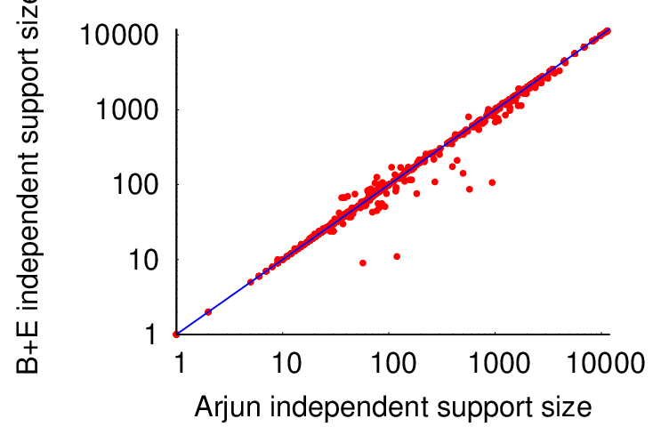
At this point, one may wonder about the size of independent supports computed by $\mathsf{Arjun}$, $\mathsf{MIS}$, and and $\mathsf{B+E}$. To this end, we present scatterplot of the size of independent support found by $\mathsf{Arjun}$, $\mathsf{MIS}$, and $\mathsf{B+E}$ in Figure 3. Since $\mathsf{Arjun}$ found an independent support for a greater number of instances within the 5000s time limit, we only show the size of independent supports for instances that both $\mathsf{Arjun}$ and $\mathsf{B+E}$ (resp. $\mathsf{Arjun}$ and $\mathsf{MIS}$) finished on, for a true apples-to-apples comparison.

To understand the impact of $\mathsf{ExplicitSearch}$ and $\mathsf{IntegratedImplicit}$, we present the runtime performance of different versions of $\mathsf{Arjun}$ in Figure 4. The curve “$\mathsf{Arjun}$ w/o $\mathsf{IntegratedImplicit}$” refers to the version of $\mathsf{Arjun}$ with $\mathsf{SimpleSearch}$ instead of $\mathsf{IntegratedImplicit}$, while “$\mathsf{Arjun}$ w/o $\mathsf{ExplicitSearch}$” refers to the version of $\mathsf{Arjun}$ without explicit definability-based identification. We make two observations: (1) both phases play a crucial role in the performance of the tool, and (2) the impact of $\mathsf{IntegratedImplicit}$ is higher than that of $\mathsf{ExplicitSearch}$.

Figure 5 shows the cactus plot of $\mathsf{ApproxMC3}$, $\mathsf{ApproxMC4}$, $\mathsf{MIS}$+$\mathsf{ApproxMC4}$, and $\mathsf{Arjun}$+$\mathsf{ApproxMC4}$ (cumulative time). Here, $\mathsf{Arjun}$ or ${\mathsf{MIS}}$ was first ran on the benchmark, and the resulting independent support was provided to $\mathsf{ApproxMC4}$. $\mathsf{Arjun}$+$\mathsf{ApproxMC4}$ could count 1596 instances while $\mathsf{ApproxMC4}$ and $\mathsf{MIS}$+$\mathsf{ApproxMC4}$ could only count 1209 and 1262 instances, respectively within the same 5000s timeout. Overall, we observe an improvement of 334 instances. To put this into context, we also plot the curve corresponding to $\mathsf{ApproxMC3}$, which demonstrates significant improvement $\mathsf{Arjun}$ provides relative to $\mathsf{ApproxMC4}$ vs $\mathsf{ApproxMC3}$. Solving speed improvement is substantial: with a timeout of only 34 seconds, $\mathsf{Arjun}$+$\mathsf{ApproxMC4}$ could solve as many instances as $\mathsf{ApproxMC4}$ on its own under 5000 seconds.

To further compare the runtime on a per instance basis, we present the scatter plot of $\mathsf{Arjun}$+$\mathsf{ApproxMC4}$ vis-a-vis $\mathsf{MIS}$+$\mathsf{ApproxMC4}$ in Figure 6. We observe that on a per instance basis $\mathsf{Arjun}$+$\mathsf{ApproxMC4}$ is almost always faster than $\mathsf{MIS}$+$\mathsf{ApproxMC4}$.

This demonstrates the importance of efficient computational technique that can find small independent support. Recall that $\mathsf{ApproxMC4}$ adds XORs over the independent support in order to perform approximate counting. Hence, a smaller independent support leads to faster propagation and on average smaller conflict clauses.

Figure 7 shows the cactus plot of $\mathsf{UniGen2}$, $\mathsf{UniGen3}$, $\mathsf{MIS}$+$\mathsf{UniGen3}$, and $\mathsf{Arjun}$+$\mathsf{UniGen3}$ (cumulative time). Overall, $\mathsf{Arjun}$+$\mathsf{UniGen3}$ samples 1354 instances, 298 more than $\mathsf{MIS}$+$\mathsf{UniGen3}$ within the same 5000s timeout. To put such a performance improvement into context, observe that the difference between $\mathsf{UniGen2}$ and $\mathsf{UniGen3}$ in terms of number of sampled instances is significantly less than $\mathsf{MIS}$+$\mathsf{UniGen3}$ vs $\mathsf{Arjun}$+$\mathsf{UniGen3}$.

References

- [1] Baluta, T., Shen, S., Shinde, S., Meel, K.S., Saxena, P.: Quantitative verification of neural networks and its security applications. In: Proceedings of the 2019 ACM SIGSAC Conference on Computer and Communications Security. pp. 1249–1264 (2019)
- [2] Beth, E.W.: On Padoa’s method in the theory of definition. In: Journal of Symbolic Logic 21. pp. 194–195. No. 2 (1956)
- [3] Chakraborty, S., Meel, K.S., Vardi, M.Y.: A scalable and nearly uniform generator of SAT witnesses. In: Proc. of CAV. pp. 608–623 (2013)
- [4] Chakraborty, S., Meel, K.S., Vardi, M.Y.: A scalable approximate model counter. In: Proc. of CP. pp. 200–216 (2013)
- [5] Chakraborty, S., Meel, K.S., Vardi, M.Y.: Balancing scalability and uniformity in SAT witness generator. In: Proc. of DAC. pp. 1–6 (2014)
- [6] De Morgan, A.: Trigonometry and Double Algebra. Taylor, Walton, and Malbery, London (1849)
- [7] Duenas-Osorio, L., Meel, K.S., Paredes, R., Vardi, M.Y.: Counting-based reliability estimation for power-transmission grids. In: Proc. of AAAI (2017)
- [8] Eén, N., Sörensson, N.: An extensible SAT-solver. In: International conference on theory and applications of satisfiability testing. pp. 502–518. Springer (2003)
- [9] Ermon, S., Gomes, C., Sabharwal, A., Selman, B.: Low-density parity constraints for hashing-based discrete integration. In: International Conference on Machine Learning. pp. 271–279. PMLR (2014)
- [10] Gomes, C.P., Hoffmann, J., Sabharwal, A., Selman, B.: Short XORs for model counting: from theory to practice. In: International Conference on Theory and Applications of Satisfiability Testing. pp. 100–106. Springer (2007)
- [11] Ivrii, A., Malik, S., Meel, K.S., Vardi, M.Y.: On computing minimal independent support and its applications to sampling and counting. Constraints pp. 1–18 (2015). https://doi.org/10.1007/s10601-015-9204-z
- [12] Lagniez, J.M., Lonca, E., Marquis, P.: Improving model counting by leveraging definability. In: IJCAI. pp. 751–757 (2016)
- [13] Lagniez, J.M., Lonca, E., Marquis, P.: Definability for model counting. Artificial Intelligence 281, 103229 (2020)
- [14] Liffiton, M.H., Sakallah, K.A.: Algorithms for computing minimal unsatisfiable subsets of constraints. Journal of Automated Reasoning 40(1), 1–33 (2008)
- [15] Malik, S., Zhao, Y., Madigan, C.F., Zhang, L., Moskewicz, M.W.: Chaff: Engineering an efficient SAT solver. Design Automation Conference pp. 530–535 (2001). https://doi.org/http://doi.ieeecomputersociety.org/10.1109/DAC.2001.935565
- [16] Meel, K.S., Akshay, S.: Sparse hashing for scalable approximate model counting: theory and practice. In: Proceedings of the 35th Annual ACM/IEEE Symposium on Logic in Computer Science. pp. 728–741 (2020)
- [17] Meel, K.S., Soos, M.: Model counting and uniform sampling instances. https://doi.org/10.5281/zenodo.3793090 (May 2020). https://doi.org/10.5281/zenodo.3793090
- [18] Naveh, Y., Emek, R.: Random Stimuli Generation for Functional Hardware Verification as a CP Application. In: Proc. of CP. Lecture Notes in Computer Science, vol. 3709, pp. 882–882. Springer (2005)
- [19] Ostrowski, R., Grégoire, É., Mazure, B., Sais, L.: Recovering and exploiting structural knowledge from CNF formulas. In: Proc. of CP. Lecture Notes in Computer Science, vol. 2470, pp. 185–199. Springer (2002)
- [20] Padoa, A.: Essai d’une théorie algébrique des nombres entiers, précédé d’une introduction logique à une theorie déductive quelconque. In: Bibliothèque du Congrès international de philosophie. vol. 3, pp. 309–365 (1901)
- [21] Pipatsrisawat, K., Darwiche, A.: A lightweight component caching scheme for satisfiability solvers. In: Marques-Silva, J., Sakallah, K.A. (eds.) SAT 2007. pp. 294–299. Springer (2007)
- [22] Roy, J.A., Markov, I.L., Bertacco, V.: Restoring circuit structure from sat instances. In: IWLS. pp. 361–368 (2004)
- [23] Sashittal, P., El-Kebir, M.: Sharptni: counting and sampling parsimonious transmission networks under a weak bottleneck. bioRxiv p. 842237 (2019)
- [24] Sharma, S., Roy, S., Soos, M., Meel, K.S.: Ganak: A scalable probabilistic exact model counter. In: IJCAI. vol. 19, pp. 1169–1176 (2019)
- [25] Slivovsky, F.: Interpolation-based semantic gate extraction and its applications to QBF preprocessing. In: International Conference on Computer Aided Verification. pp. 508–528. Springer (2020)
- [26] Soos, M., Gocht, S., Meel, K.S.: Tinted, detached, and lazy CNF-XOR solving and its applications to counting and sampling. In: International Conference on Computer Aided Verification. pp. 463–484. Springer (2020)
- [27] Soos, M., Meel, K.S.: Bird: Engineering an efficient CNF-XOR sat solver and its applications to approximate model counting. In: Proc. of the AAAI (2019)
- [28] Valiant, L.G.: The complexity of enumeration and reliability problems. SIAM Journal on Computing 8(3), 410–421 (1979)
Appendix 0.A Appendix
0.A.1 Fast Syntactic AND Gate Recovery From a CNF
When trying to perform syntactic AND recovery from a CNF, we are looking for the following pattern in the CNF. First, there must exists a set of binary clauses
and secondly, a longer clause
These together indicate the AND gate
The currently best published work on syntactic gate recovery from a CNF is by [22]. It presents a flexible algorithm to discover a wide variety of gates. However, a faster algorithm is possible if only AND gates need to be discovered. To this end, we developed shown in Algorithm 5.
Algorithm 5 works as follows. First, it clears out the return value , then calls for all possible output literals . In turn, in Algorithm 6 finds all possible AND gates that can be an output of. To this end, it marks the literals that is in binary clauses with. If no literal has been marked, it is not possible to find any AND gates with as an output in a purely syntactic way and the algorithm early aborts. Otherwise, it goes through all the clauses that is part of, and ensures that all other literals in the clause have a marking on their opposite polarity. If it finds such a clause, it saves the clause and literal pair as a new AND gate. Finally, it clears up the markings it has set.
0.A.2 The Algorithm of MiniSat
The pseudocode sketch for function is shown in Algorithm 7, presented in the style of the seminal MiniSat paper by [8].
The algorithm makes use of the following standard data structures and subroutines:
-
current decision level, incremented every time the subroutine is called.
subroutine to perform the backtracking to the level given as the argument.
value of the literal assigned currently. If a variable is assigned True, then returns True while returns False.
Performs the conflict analysis and adds the learnt clause
returns True or False based on the underlying restart policy
We now provide a quick overview of (). First observe that there is an outer while loop 1– 27 and the algorithm exits either when a satisfying assignment is found or it can conclude that the formula is UNSAT. As noted earlier, we run CDCL loops up to a fixed number of conflicts. From our perspective, we focus on the lines 3– 10 wherein the algorithm inserts the assumptions into its decision queue as if it was a decision. Note that subsequent to each insertion of an assumption, a full, until-fixedpoint is called, on line 18.