Interpolation and approximation via Momentum ResNets and Neural ODEs

In the last decades, ever-increasing computational power has enabled the development of Neural Networks with complex architectures to perform in different tasks in Machine Learning. However, the power of these tools is often measured by engineering experiments, with no deep analysis of the model’s potential and limits. In this paper, we analyse interpolation and approximation properties of two models involving memory terms in some fundamental tasks of Supervised Learning, namely the representation of functions. We will show in particular that these models have advantages with respect to the Neural ODEs previously studied in [17].

We first study the continuous-layer version of Momentum ResNets, recently proposed in [18], with a ReLU activation function. Precisely, the Neural ODE we investigate is

where $x(t)\in\mathbb{R}^{d}$, $\sigma:\mathbb{R}\to\mathbb{R}$ is the ReLU activation function, $a,w\in L^{\infty}((0,T),\mathbb{R}^{d})$ and $b\in L^{\infty}((0,T),\mathbb{R})$. We will prove an interpolation result and the universal approximation property.

Then, we introduce a class of Neural ODEs with auxiliary states, $p$, representing the memory of the system, namely

where $x(t)\in\mathbb{R}^{d}$ and $p(t)\in\mathbb{R}^{d_{p}}$, $C\in L^{\infty}((0,T);\mathbb{R}^{d\times d_{p}})$, $W,A\in L^{\infty}((0,T);\mathbb{R}^{d\times d})$, $d,b_{1},b_{2}\in L^{\infty}((0,T);\mathbb{R}^{d})$, $f\in L^{\infty}((0,T);\mathbb{R})$ and $\boldsymbol{\vec{\sigma}}:\mathbb{R}^{d}\to\mathbb{R}^{d}$ is the componentwise application of the activation function. We will prove an interpolation result for maps giving a continuous parameterization of time-dependent functions, precisely

with $\Omega$ a bounded set. We first investigate the ability of this type of NODEs to interpolate samples of $M$ for all times in $(0,T)$, and then to approximate $M$ through the flow of (1.2). These correspond, respectively, to the properties of simultaneous tracking controllability and universal tracking approximation.

Supervised Learning is the branch of Machine Learning that studies how to learn a function based on a finite collection of samples. To obtain a solution for these problems, one typically uses a parameterized class of functions; then, the parameters that correspond to the best candidate in the class are found through optimization techniques.

Neural Networks (NN) [12] are a common choice of such parameterized classes of functions. In this article, we focus on continuous layer versions of Residual Neural Networks (ResNets), introduced in [9], which have been observed to outperform of previous classes [11], especially in tasks where a time structure is present, like in text and video recognition. ResNets are a collection of $N_{l}\in\mathbb{N}$ consecutive layers of neurons, where the initial data $\{x_{i}\}_{i=1}^{N}$, $N\in\mathbb{N}$, are transformed following a relation of the type

Here, $\omega_{k}$ are the parameters to be chosen. The peculiarity of ResNets with respect to previous deep NN architectures is the presence of an inertia term $x_{k}$ in the definition of the term $x_{k+1}$. To fix the ideas, for the Momentum ResNets, $g:\mathbb{R}^{3d+1}\to\mathbb{R}^{d}$ it is going to be

where $\omega:=\left\{w_{k},a_{k},b_{k}\right\}_{k=1}^{N_{\mathrm{l}}}$ are parameters such that $w_{k},a_{k}\in\mathbb{R}^{d}$ and $b_{k}\in\mathbb{R}$, and $\langle\cdot,\cdot\rangle$ denotes the scalar product. The function $\sigma$ is the so-called activation function. When not stated otherwise, $\sigma:\mathbb{R}\to\mathbb{R}$ will denote the Rectified Linear Unit (ReLU) defined by

In practical situations, the controls are found through optimization techniques. In the context of continuous-layer models, this is equivalent to solve optimal control problems, see [1, 6, 20].

The ResNet architecture (1.4) can be seen as an Euler discretization of a continuous time model, see [2, 6, 8, 19]. In fact, as the number of layers $N_{l}$ goes to infinity, one can understand (1.4) as the discretization of the ODE

as was done in [19]. By reading the parameters $\omega(t)$ as time-dependant functions, we can solve the approximation problems from an ODE point of view. In fact, for all times $T\geqslant 0$ there exists a flow

which is the solution to the equation (1.9) at $T$ for the initial condition $x$ and functions $w$, $a$ and $b$. We will read $w$, $a$ and $b$ as the controls of the equation (1.9). We will ask if the flow (1.8) at a certain time $T$ is able to approximate a desired function for suitable controls.

One basic question to address is if a NN is able to interpolate any set of samples of the target function; that is, given a sample of initial points $\{x_{i}\}_{i=1}^{N}\subset\mathbb{R}^{d}$, with $d$ and $N$ in $\mathbb{N}$, and of target points $\{y_{i}\}_{i=1}^{N}\subset\mathbb{R}^{d}$, we ask if there exist a function $\omega$ such that for all $i=1,\dots,N$ we have that $\phi_{T}(x_{i},\omega)=y_{i}$. This is a simultaneous control problem [14, 15]. Along the paper, interpolation is equivalent to a simultaneous control problem. This issue has been considered, for instance, in [17] through explicit constructions and in [3] using Lie Bracket techniques.

Another important theoretical question to ask is if, given a function $f:\Omega\subset\mathbb{R}^{d}\to\mathbb{R}^{d}$, $d\in\mathbb{N}$, $\Omega$ a bounded set, a NN is able to approximate $f$ as accurately as desired on $\Omega$, for example in the $L^{2}$ norm. This property of the NN is called universal approximation, see for instance [4, 5, 7, 10, 13, 16].

Now we turn our attention to being able to approximate more general maps, as the one in (1.3), through a Neural ODE. We consider a collection of samples of $M$, $\{y_{i}=M(x_{i})\}_{i=1}^{N}$ with $y_{i}\in C^{0}((0,T);\mathbb{R}^{d})\cap BV((0,T);\mathbb{R}^{d})$. We say that the dynamics (1.2) is simultaneously tracking-controllable if there exist a control functions $\omega$ such that the associated flow $\phi_{t}(x_{i},\omega)$ is close to $y_{i}(t)$ for every $i$ and $t\in[0,T]$. The tracking controllability has been studied in some problems in control of PDEs, for instance see [1].

We will also discuss the universal tracking approximation, where the goal is to approximate the map $M$ with the flow given by the NODE (1.2).

In [17], the authors considered the NODE

that from now on, to make a clear distinction, we will call a first-oder NODE. When the initial data and the targets are in $\mathbb{R}^{d}$, the dynamics of (1.9) is not able to interpolate exactly any set of points. This happens because, by uniqueness of the solution of (1.9), one cannot drive two distinct points to the same target; so, if two targets coincide, there cannot be simultaneous exact controllability.

In the recent paper [18], the authors proposed a new model of continuous layer ResNets. Precisely, instead of (1.9), they use the equation with parameters $\theta\in\mathbb{R}^{d\times d}$ given by

which is called a Momentum ResNet. A major difference with respect to NODEs is that two points can share the same position and be distinguished by their velocity. Moreover, Momentum ResNets allows the authors of [18] to use a backpropagation algorithm requiring less memory with respect to the NODEs. In this framework, the parameter $\varepsilon$ acts as a measure of the memory of the system, seen as the dependence on previous layers. When $\varepsilon\to 0$, one recovers the NODE. Regarding the fundamental properties of the Momentum ResNets, the authors investigate the class of functions that can be recovered via the Momentum ResNets with a linear function $g(x)=\theta\,x$, $\theta\in\mathbb{R}^{d\times d}$, proving that they can recover diagonalizable matrices satisfying a certain condition on their eigenvalues.

In this paper, the first model we investigate is the Momentum Resnet

with $\sigma$ as in (1.6) and $w$, $a\in L^{\infty}((0,T);\mathbb{R}^{d})$, and $b\in L^{\infty}((0,T);\mathbb{R})$. Notice that, for the sake of simplicity of the mathematical dissertation, we took $\varepsilon=1$, thus taking into account the case of a strong memory dependence. However, the dynamical properties we will employ are not dependent on this parameter. We are going to investigate simultaneous controllability and universal approximation in $L^{2}$ for the Momentum ResNets as in (1.10). Following the intuitions in [17], our proofs are relying on constructive arguments arising from the analysis of the exact dynamics of (1.10).

We stress that Momentum ResNets can also be seen as memory like models. Indeed, the problem in (1.10) is equivalent to

where we see that the past influences the dynamics of the system. Notice that we will have dependences on at least two layers when considering the discretization of the second derivative of the ODE.

A different way to include memory in the system is to have some auxiliary states playing the role of memory terms in the architecture. We will consider memory models of the form

where $x\in\mathbb{R}^{d}$ is the state variable and $p\in\mathbb{R}^{d_{p}}$, $d_{p}\in\mathbb{N}$, is considered the memory variable. As for the ResNets, we will focus on a continuous time version of (1.12), precisely

with $a$, $b$, $w$ as before, $c,u,d\in L^{\infty}((0,T);\mathbb{R}^{d})$, and $f\in L^{\infty}((0,T);\mathbb{R})$. Note that, if we set the initial memory to be $0$, the equation can be written as:

Models with memory states, even continuous ones, are not new in the literature, see [21] and the references therein. By using the properties of the first-order NODEs (1.9) analysed in [17], it will be easy to deduce simultaneously controllability and the universal approximation property for (1.13).

The simultaneous controllability for (1.13) allows to control both the state and the memory variable. This property is, for us, crucial to prove the simultaneous tracking controllability and universal tracking approximation. However, in order to do so, we need to extend the system (1.13) to a more general one, given in (1.2). The model (1.2) (as well as (1.13)) could be understood as a Neural ODE in a higher dimensional space, in which we only consider some components as the state. In particular, we will consider the components of $p$ as memory states. We will refer to (1.2) as a Memory NODE, to make a even clearer distinction with respect to the first-order NODE in (1.9).

We are able to prove simultaneous tracking controllability for Memory NODEs; in particular, we will be able to control the trajectories on an interval $[0,T]$ for any time horizon $T>0$. In our proof, the price to pay to obtain the simultaneous tracking controllability property is to consider a minimum dimension on the memory. In fact, we need $p\in\mathbb{R}^{d_{p}}$ with $d_{p}=2d$, which means that we have to consider a system that has bigger size with respect to (1.10) and (1.9). Moreover, also the controls take values in a higher dimensional space. However, we do not know if this is a fundamental requirement or if it is just technical. Given the results of simultaneous tracking control and universal approximation, the universal tracking approximation follows as a corollary.

The paper is organized as follows:

• •

  In Section 2, we state in detail the results concerning Momentum ResNets, and we will discuss the dynamical properties that allows us to prove the simultaneous controllability and the universal approximation theorem. The proofs for these theorems are in Appendix A.

• •

  In Section 3, we state the main results concerning Memory NODEs, the simultaneous control of the state-memory pair, the tracking simultaneous controllability, and we will prove the universal tracking approximation. The complete proofs for these theorems are in Appendix B.

• •

  In Section 4, we will complete the study providing numerical simulations for those models in the discussed tasks. Specifically, we applied the systems to the case of indicator and sinusoidal functions.

• •

  We will give some final comments in Section 5.

Let us briefly describe the different types of flows that allow us to guarantee the results. For doing so, we will take controls $a,\ w\in\mathbb{R}^{d}$ and $b\in\mathbb{R}$; in this Subsection, we consider them to be time independent. More specifically, we will analyze a component at a time; fix $i\in\{1,...,d\}$ and consider $a$ in the form $a^{(k)}=\delta_{i,k}$, where $\delta_{i,k}$ is the Kronecker delta. By a simple translation, it is enough to understand the flows for $b=0$. The ODE (1.10) can be rewritten as:

which component-wise is equivalent to

Of all possible cases, take into account these three:

1. 1.

   $\boxed{\ddot{x}^{(i)}+\dot{x}^{(i)}=0}$ Thus, we analyse the dynamics in the inactive hyperplane of the activation function. Denoting $\dot{x}=p$, the solution is

   $$\begin{array}[]{l}x^{(j)}(t)=x^{(j)}(0)+(1-e^{-t})(p^{(j)}(0))\\ p^{(j)}(t)=p^{(j)}(0)e^{-t}\end{array}$$

   (2.4)

2. 2.

   $\boxed{\ddot{x}^{(i)}+\dot{x}^{(i)}+wx^{(i)}=0}$ It corresponds to the case in which we are in the side of the space in which the activation function is not zero and $j=i$. The dynamics is

   $$\begin{pmatrix}x\\ p\end{pmatrix}^{\prime}=\mathcal{A}\begin{pmatrix}x\\ p\end{pmatrix}=\begin{pmatrix}0&1\\ -w&-1\end{pmatrix}\begin{pmatrix}x\\ p\end{pmatrix},$$

   where the eigenvalues and eigenvectors of the matrix $\mathcal{A}$ are given by

   $$\lambda_{\pm}=\frac{1}{2}\pm\sqrt{\frac{1}{4}-w},\ v_{\pm}=\begin{pmatrix}1\\ -\frac{1}{2}\pm\sqrt{\frac{1}{4}-w}\end{pmatrix}.$$

   Here, three cases arise

   1. (a)

      if $w\in(0,1/4)$, the origin is an attractor;

   2. (b)

      if $w\geqslant 1/4$, the dynamics behaves as a damped oscillator;

   3. (c)

      if $w<0$, the origin is a saddle point.

3. 3.

   $\boxed{\ddot{x}^{(j)}+\dot{x}^{(j)}+w^{(j)}x^{(i)}=0}$ with $i\neq j$. Consider $w^{(j)}\neq 0$, and assume that the quantity $q=w^{(i)}x^{(i)}$ is time independent. Then, the solution is

   $$\begin{split}x^{(j)}(t)&=x^{(j)}(0)+(1-e^{-t})p^{(j)}(0)\\ &+q(t-1+e^{-t}),\\ p^{(j)}(t)&=e^{-t}p^{(j)}(0)+q(1-e^{-t}).\end{split}$$

   (2.5)

The control strategy will consist on splitting the time interval $(0,T)$ in two $(0,T/2)$ and $(T/2,T)$ and each interval is also divided in several subintervals and proceed interatively. In $(0,T/2)$ the goal will be to act appriopiately on the first component of each point whereas in $(T/2,T)$ the objective will be to act on the remaining components for each point. The argument is similar in both intervals, very schematically the procedure is:

1. 1.

   In each subinterval a specific point is chosen

2. 2.

   One chooses a control that will perturb the dynamics of several points with the goal of modifying appropriately the trajectory of the chosen point so that the free dynamics will bring the point to its target.

3. 3.

   We will make use of the fact that the control acts only in half space to not perturb the trajectories that have already been appropriately controlled.

Setting $x(0)$ and $p(0)$ in (2.4) as the output of (2.5) one arrives at:

One can realize that, for any $T>t>0$, the expression above is a line, and therefore, one can always choose $q$ so that at the time $T$ the state is at the desired position.

The universal approximation follows with the same arguments than in [17]:

1. 1.

   Consider a suitably fine mesh made out of hyperrectangles, and apply a compression to each rectangle.

2. 2.

   By Theorem 2.1, we control a point of each compressed rectangle to its target. We can then conclude by continuity of the ODE with respect to the initial data.

We point out that for $w\in(0,1/4)$ we can generate a compressive flow. One can see that using the eigenvectors of $\mathcal{A}$ one can define an invariant region inside $\{x^{(i)}\geqslant 0\}$ such that all the trajectories converge to the origin $(0,0)$, see Figure 1.

Let $d,d_{p}\in\mathbb{N}$ and consider the following ODE system:

We will call $x$ the state component of the system and $p$ the memory component.

Our first goal is to be able to simultaneously control both the state and the memory at the final time for any target configuration with distinct state-memory pairs. The fact of being able to control also the memory will be key for the simultaneous tracking control problem that we will describe later on.

The proof of Proposition 3.1 makes use of an extension of the techniques developed in [17] for the control of

In [17], using Cartesian flows, the authors can prove a simultaneous control result for any $d\geqslant 2$.

In this proof, we have two aspects to deal with. Firstly, notice that the field of the memory variable only depends on the state component, so, even if similar mechanisms to the case of first order the Neural ODE (1.9) can be applied, the intrinsic limitation of only depending on the state components should be discussed. Secondly, the dimensions $d$ and $d_{p}$ might not coincide. It would be certainly simpler to consider $d=d_{p}$, but as we shall see later on, the dimension of the memory plays a crucial role in the approximate simultaneous tracking controllability.

Let us briefly remind some key features of the control of the Neural ODE for $d=2$ shown in [17]. The dynamics is

By using flows of these two types (see Figure 3),

and

one can prove the approximate simultaneous controllability (see also Section 2 for Momentum ResNets). As one can see from Figure 3, the flows associated to (3.3) and (3.4) freeze one side of the hyperplane, selected by $\langle a,x\rangle+b=0$, and cause a parallel movement in the nonfrozen half space.

The main feature is that, in the equations in (3.3) and (3.4), the evolution of one component, say $x^{(1)}$ does not depend on $x^{(1)}$ itself, but on the other components. For this reason, even with the considered system (3.1), the evolution of the memory component does not depend on itself, so we can still have a simultaneous controllability result. In the Appendix B, we will provide a proof of the simultaneous control result for the Neural ODE.

The proof is postponed into the Appendix B.1

The goal of this section is to show how by the memory can help to obtain a simultaneous tracking controllability property.

We will consider a finite collection of samples of a continuous function $M$,

That is, we have a dataset of the form

For being able to approximate the map $M$, we will consider an extension of (3.1). Instead of considering a scalar product between two vectors $\langle a,b\rangle$ or $\langle c,p\rangle$ in the state equation, we will consider a matrix vector product. Precisely, we take

where $b_{1},b_{2}\in L^{\infty}((-\tau,T);\mathbb{R}^{d})$,
$W,A\in L^{\infty}((-\tau,T);\mathbb{R}^{d\times d})$, $C\in L^{\infty}((-\tau,T);\mathbb{R}^{d\times d_{p}})$. Note that the memory component of the system is the same as in (3.1). Again, notice that (3.5) can be rewritten as:

On the other hand, for suitable controls, the system (3.5) has the same flows as (3.1). In particular, Theorem 3.1 also holds for (3.5) (and also the universal approximation of [17]).

The following theorem is the simultaneous tracking controllability, that we are able to achieve by taking the dimension of the memory as, at least, the double of the state dimension.

In the interval $(-\tau,0)$, we use the controls to prepare the memory variables before the simultaneous tracking control process. We will postpone the proof in the Appendix B.2, giving only some flavour here.

The proof of the theorem is based on the following two observations. We will consider $d_{p}=2d$; from here on, we will make an abuse of notation by writing $p=(p^{(1)},p^{(2)})$ where $p^{(1)},p^{(2)}\in\mathbb{R}^{d}$.

1. 1.

   We begin by approximating linear maps of the form $y_{i}=P_{i}t+B_{i}$ with $P_{i}$, $B_{i}\in\mathbb{R}^{d}$. For every $i\in\{1,...,N\}$ let $B_{i}$ be the targets for the state for Theorem 3.1 and $p_{i}$ the targets for the memory to be found hereafter. Then, consider $A=0$, $b_{1}=0$, $W=I_{d}$; the dynamics of the state equation is

   $$x^{\prime}=\boldsymbol{\vec{\sigma}}(Cp)+b_{2}.$$

   We choose $C=(I_{d}|0)$; since we consider $\sigma$ to be the ReLU, we reduce the problem to finding $b_{2}\in\mathbb{R}^{d}$ such that

   $$p_{i}^{(1)}=P_{i}-b_{2}\in\mathbb{R}_{+}^{d}\qquad i\in\{1,...,N\},$$

   which is always possible. Then the dynamics reads

   $$x^{\prime}=P_{i},\quad x(0)=B_{i}.$$

   The solutions to the latter are precisely $P_{i}t+B_{i}$ for all $i\in\{1,...,N\}$.

2. 2.

   The second point is to use the first and second component of the memory in an alternate manner. We will first approximate the target functions by means of piecewise linear functions of time, as Figure 4 shows. Then, we will use an alternate strategy, while we are using the first component of the memory to control the system, we will reconfigure the second component to be prepared for the next interval as Figure 5.

For the first problem, we choose a function

precisely the characteristic function of a circle centred in $(0,0)$. We take $N=100$ random samples of it. Then, we use these samples to train a Neural ODE (see Figures 6 and 7) and a Momentum ResNet (see Figure 8 and 9) and observe the differences.

We employ a least-squares approach by minimizing

where by $\omega$ we understand the controls as well as the projection $P$, i.e. $\omega=(a,w,P,b)$ belongs to

$x_{i}(T;\omega)$ is the solution at time $T$ of either a Momentum ResNet as in (1.1) with initial datum $(x_{i},0)$ or a Neural ODE

For both models, we take a sigmoid activation function.

Being $\mathcal{S}$ a set and $\chi_{\mathcal{S}}$ the characteristic function of such set, we measure the generalization error by means of the $L^{1}$ norm, i.e.

where with an abuse of notation we denote $P\phi_{T}$ both the solution of the Neural ODE and the projection to the position of the solution of the Momentum ResNet.

At the final time, a suitable hyperplane $H$ separates the training points, determining whether their image is 0 or 1. That is, this hyperplane fix the decision boundary. Since the map

is a homeomorphism, we have that $(\phi_{T})^{-1}(H)$ is topologically equivalent to a hyperplane. In particular, the decision boundary for a first-order NODE cannot have the same topology of the boundary of the circle, which is a closed curve. So, the decision boundary touches the border of the square in Figure 6, misrepresenting some points that are far from the border of the circle.

On the other hand, for Momentum ResNets, the decision boundary is determined by a projection only on the state variable. This means that the decision boundary is not necessarily topologically equivalent to a hyperplane. From the simulations, we see that the Momentum ResNet has been able to capture the topology of the set $\mathcal{S}$ and to perform the task with smaller error.

We will consider a function

precisely $M(x)=\sin(xt)$. We take a sample of $5$ random points $x_{i}\in(0,1)$ and define

We minimize the functional

where $x_{i}(t;\omega)$ is the solution of

with $a,\ w,\ d$, $b_{1},\ b_{2}\in L^{\infty}((-\tau,T);\mathbb{R})$ and $c,\ u\in L^{\infty}((-\tau,T);\mathbb{R}^{2})$.

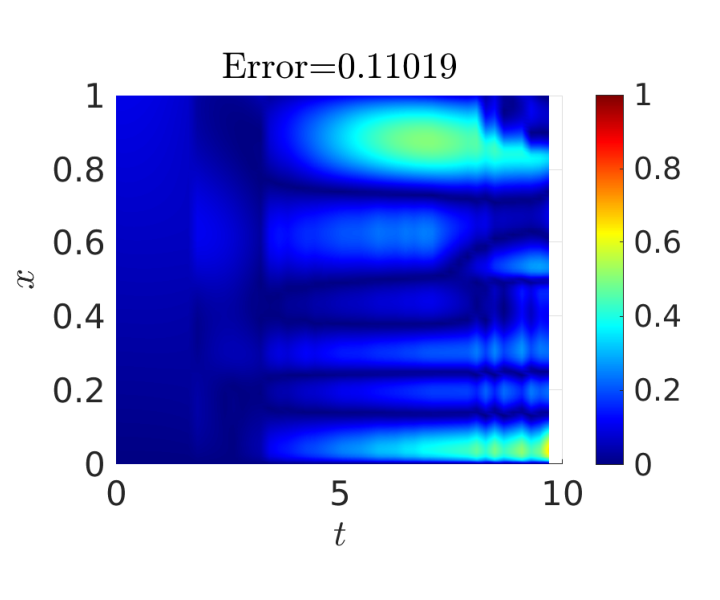
We get an error smaller than 0.063529 for the simultaneous tracking and an error of 0.11019 for the overall universal approximation.

References

- [1] J. A. Bárcena-Petisco. Optimal control for neural ode in a long time horizon and applications to the classification and simultaneous controllability problems. 2021.
- [2] R. T. Chen, Y. Rubanova, J. Bettencourt, and D. Duvenaud. Neural ordinary differential equations. arXiv preprint arXiv:1806.07366, 2018.
- [3] C. Cuchiero, M. Larsson, and J. Teichmann. Deep neural networks, generic universal interpolation, and controlled odes. SIAM Journal on Mathematics of Data Science, 2(3):901–919, 2020.
- [4] G. Cybenko. Approximation by superpositions of a sigmoidal function. Mathematics of control, signals and systems, 2(4):303–314, 1989.
- [5] I. Daubechies, R. DeVore, S. Foucart, B. Hanin, and G. Petrova. Nonlinear approximation and (Deep) ReLU networks. Constructive Approximation, pages 1–46, 2021.
- [6] C. Esteve, B. Geshkovski, D. Pighin, and E. Zuazua. Large-time asymptotics in deep learning. arXiv preprint arXiv:2008.02491, 2020.
- [7] I. Gühring and M. Raslan. Approximation rates for neural networks with encodable weights in smoothness spaces. Neural Networks, 134:107–130, 2021.
- [8] E. Haber and L. Ruthotto. Stable architectures for deep neural networks. Inverse Problems, 34(1):014004, 2017.
- [9] K. He, X. Zhang, S. Ren, and J. Sun. Deep residual learning for image recognition. In Proceedings of the IEEE conference on computer vision and pattern recognition, pages 770–778, 2016.
- [10] K. Hornik, M. Stinchcombe, and H. White. Multilayer feedforward networks are universal approximators. Neural networks, 2(5):359–366, 1989.
- [11] A. Kolesnikov, L. Beyer, X. Zhai, J. Puigcerver, J. Yung, S. Gelly, and N. Houlsby. Big transfer (bit): General visual representation learning. In Computer Vision–ECCV 2020: 16th European Conference, Glasgow, UK, August 23–28, 2020, Proceedings, Part V 16, pages 491–507. Springer, 2020.
- [12] Y. LeCun, Y. Bengio, and G. Hinton. Deep learning. nature, 521(7553):436–444, 2015.
- [13] Q. Li, T. Lin, and Z. Shen. Deep learning via dynamical systems: An approximation perspective. arXiv preprint arXiv:1912.10382, 2019.
- [14] J.-L. Lions. Exact controllability, stabilization and perturbations for distributed systems. SIAM review, 30(1):1–68, 1988.
- [15] J. Lohéac and E. Zuazua. From averaged to simultaneous controllability. In Annales de la Faculté des sciences de Toulouse: Mathématiques, volume 25, pages 785–828, 2016.
- [16] A. Pinkus. Approximation theory of the mlp model in neural networks. Acta numerica, 8:143–195, 1999.
- [17] D. Ruiz-Balet and E. Zuazua. Neural ode control for classification, approximation and transport, 2021.
- [18] M. E. Sander, P. Ablin, M. Blondel, and G. Peyré. Momentum residual neural networks. arXiv preprint arXiv:2102.07870, 2021.
- [19] E. Weinan. A proposal on machine learning via dynamical systems. Communications in Mathematics and Statistics, 5(1):1–11, 2017.
- [20] C. E. Yagüe and B. Geshkovski. Sparse approximation in learning via neural odes. arXiv preprint arXiv:2102.13566, 2021.
- [21] M. Zhang, Z. McCarthy, C. Finn, S. Levine, and P. Abbeel. Learning deep neural network policies with continuous memory states. In 2016 IEEE international conference on robotics and automation (ICRA), pages 520–527. IEEE, 2016.