Second-order Cumulants Ghost ImagingPreprint: AIP/123-QED

Ghost imaging (GI) is an imaging technique based on correlation measurementPittman et al. 1995; Gao et al. 2019; Gao et al. 2017; Gatti et al. 2004; Ribeiro et al. 1994; Gatti, Brambilla, and Lugiato 2003; Meyers, Deacon, and Shih 2008; Cheng and Han 2004; Abouraddy et al. 2001; Baleine, Dogariu, and Agarwal 2006. The GI experiment has been demonstrated by Pittman et alPittman et al. 1995. Due to its surprising nonlocal feature, it was once considered as an unique phenomenon of quantum entanglementAbouraddy et al. 2001. Later, Bennink et al. presented theoretical arguments and provided experimental demonstration that GI can be performed with a classical sourceBennink, Bentley, and Boyd 2002. Compared with conventional imaging technique, GI has many advantages such as high spatial resolutionGong and Han 2012, high robustnessCheng 2009; Meyers, Deacon, and Shih 2011 and so on.

The classical limit of resolution of an optical instrument was formulated in the well-known works by Abbe and Rayleigh. This classical limit states that the resolution of an optical system is limited by diffraction on the system pupil. The resolution is determined by the point spread functions (PSF) of the system. The narrower the PSF, the better the resolutionChen et al. 2017; Wang et al. 2019. In GI system, the resolution is superior to the classical Rayleigh limitGong and Han 2012. The reason is that more nature of the light source can be distinguished by second-order coherence function than that by first-order coherence functionScully and Zubairy 1999, that is, second-order coherence properties of the light source has more information than the first-order coherence properties. Many schemes of resolution enhancement proposals have been suggested, such as compressive sensing techniqueGong and Han 2012; Du, Gong, and Han 2012, non-Rayleigh speckle fieldKuplicki and Chan 2016, low-pass spatial filter schemeChen et al. 2017; Meng et al. 2018, high-pass spatial-frequency field schemeSprigg, Peng, and Shih 2016 and so on. The cumulants of measured intensity distributions is applied to traditional imaging system and it has been proposed to narrow the PSF curve by Li et al. in 2019Li et al. 2019. The result shows that such cumulants can beat the classical Rayleigh limit. In this letter, second-order cumulants of Hanbury Brown and Twiss (HBT) intensity correlation measurement is applied to reconstruct the image of the object. The result shows that the resolution limit of GI can be enhanced by this protocol. The optical setup of GI is not changed by our scheme.

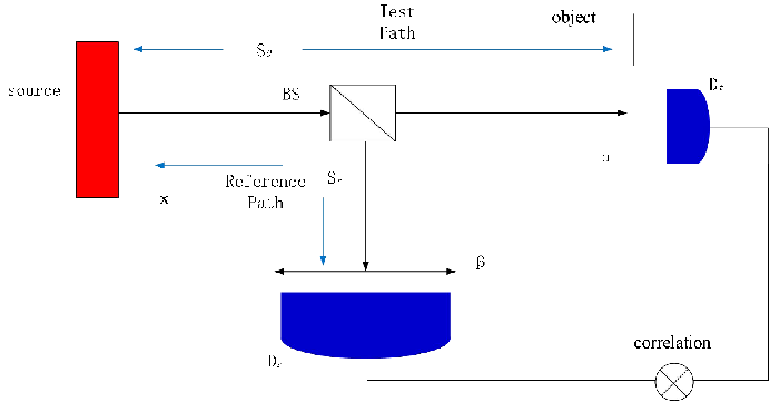
A typical GI experimental setup is shown in Fig. 1. In general, the double slit is used for measured the object, when the resolution has been studied by many researchersZeng et al. 2017; Ferri et al. 2005; Zhang et al. 2009. In this system, the source is monochromatic light with a wavelength $\lambda$. A light beam in the test path propagates to the object through an optical system with a PSF

$$h_{t}(x,\alpha)=\frac{e^{-iks_{o}}}{i\lambda s_{o}}\exp(\frac{-i\pi}{\lambda s_{o}}(x-\alpha)^{2}).$$

(1)

Here $k=\frac{2\pi}{\lambda}$, $s_{o}$ is the distance of the test path of optical system, $x$ and $\alpha$ are the transverse coordinates on the source and the object plane, respectively. If $T(\alpha)$ represents the transmission function of the object, the light field behind the object is given by

$$E(\alpha)=\int\ E(x)h_{t}(x,\alpha)T(\alpha)\,dx,$$

(2)

where $E(x)$ denotes the light field of source plane at $x$. The optical-electric current operator at the bucket detector is

$$B_{t}=\int\ E^{*}(\alpha)E(\alpha)\,d\alpha.$$

(3)

Suppose that the PSF of the reference path is $h_{r}(x,\beta)$ which has similar form as Eq. (1). The light field on the CCD plane is given by

$$E(\beta)=\int\ E(x)h_{r}(x,\beta)\,dx,$$

(4)

where $\beta$ is the transverse coordinates on the CCD plane. Thus, the optical-electric current operator at the CCD plane is

$$I(\beta)=E^{*}(\beta)E(\beta).$$

(5)

The correlation between the intensity fluctuations at the reference and test detectors is

	$\displaystyle\Delta G^{(2)}(\beta)$	$\displaystyle=\langle[I(\beta)-\langle I(\beta)\rangle][B_{t}-\langle B_{t}\rangle]\rangle=\langle\Delta I(\beta)\Delta B_{t}\rangle$
	$\displaystyle=$	$\displaystyle\int|\int\ G^{(1)}(x,x^{{}^{\prime}})T(\alpha)h_{t}(x,\alpha)h^{*}_{r}(x^{{}^{\prime}},\beta)\,dxdx^{{}^{\prime}}|^{2}d\alpha$
		$\displaystyle-\langle I(\beta)\rangle\langle B_{t}\rangle,$		(6)

where $\langle\dots\rangle$ represents the ensemble average. $G^{(1)}(x,x^{{}^{\prime}})=\langle E^{*}(x)E(x^{{}^{\prime}})\rangle$ is the first-order correlation function at source. We consider the case where the illuminated light is a point-like source which randomly and uniformly distributed on the source plane. If the light spot is located at $x_{0}$, we may have $G^{(1)}(x,x_{o})=I_{0}\delta(x-x_{0})$, where $I_{0}$ is the intensity of source. Here we also consider the distances from source to the object and the source to the CCD are same, namely $s_{r}=s_{o}=z$, we can get

$$\Delta G^{(2)}(\beta)=I_{0}^{2}\int\ |T(\alpha)|^{2}\text{sinc}^{2}(\frac{2\pi R}{\lambda z}(\alpha-\beta))\,d\alpha.$$

(7)

Where $R$ is the radius of the source plane. Obviously, the image resolution is confined by this PSF. From Eq. (7), it is $\text{sinc}^{2}(\frac{2\pi R}{\lambda z}(\alpha-\beta))$ that produces the Airy disk and the first zero of $\text{sinc}^{2}$ function leads to the resolution limit.

In general, $I_{0}$ is taken as a constant in the coventional GI under the assumption of the emitting power of the light source is perfect stable. In fact, the emitting power of the light source can not keep stable. Thus, the $\Delta G^{(2)}(\beta)$ in Eq. (7) should be substituted with $\Delta G^{(2)}(I_{0},\beta)$. The fluctuation of $I_{0}$ lead to the fluctuation of $\Delta G^{(2)}(I_{0},\beta)$. We use the concept ‘Cumulants’, which is always used in statistics, to describe the fluctuation of $\Delta G^{(2)}(I_{0},\beta)$ which have more information than $\Delta G^{(2)}(I_{0},\beta)$. The narrower PSF can be got by the cumulants than by $\Delta G^{(2)}(I_{0},\beta)$. So the resolution limit of GI can be improved. The cumulant-generating function $K(s,\beta)$ is defined.

$$K(s,\beta)=\ln(\langle\exp(s\Delta G^{(2)}(I_{0},\beta))\rangle).$$

(8)

The nth-order cumulants is given by

$$\kappa_{n}(\beta)=\frac{d^{(n)}K(s,\beta)}{ds^{(n)}}|_{s=0}.$$

(9)

We consider second-order cumulants, which can be written as

		$\displaystyle\kappa_{2}(\beta)=\langle[\Delta G^{(2)}(I_{0},\beta)-\langle\Delta G^{(2)}(I_{0},\beta)\rangle]^{2}\rangle$
		$\displaystyle=\int\kappa_{2}(\alpha,\beta)\,d\alpha+L(\beta),$		(10)

where

	$\displaystyle\kappa_{2}(\alpha,\beta)$	$\displaystyle=\langle[\Delta G^{(2)}(I_{0},\alpha,\beta)-\langle\Delta G^{(2)}(I_{0},\alpha,\beta)\rangle]^{2}\rangle$
		$\displaystyle=\langle[I_{0}^{2}-\langle I_{0}^{2}\rangle]^{2}\rangle\times|T(\alpha)|^{4}\times$
		$\displaystyle\text{sinc}^{4}(\frac{2\pi R}{\lambda z}(\alpha-\beta)),$		(11)

	$\displaystyle L(\beta)$	$\displaystyle=\int_{\alpha}\int_{\alpha^{{}^{\prime}}\neq\alpha}\ \langle[\Delta G^{(2)}(I_{0},\alpha,\beta)-\langle\Delta G^{(2)}(I_{0},\alpha,\beta)\rangle]$
	$\displaystyle[\Delta$	$\displaystyle G^{(2)}(I_{0},\alpha^{{}^{\prime}},\beta)-\langle\Delta G^{(2)}(I_{0},\alpha^{{}^{\prime}},\beta)\rangle]\rangle\,d\alpha d\alpha^{{}^{\prime}}$
	$\displaystyle=\langle$	$\displaystyle[I_{0}^{2}-\langle I_{0}^{2}\rangle]^{2}\rangle\times\int_{\alpha}\int_{\alpha^{{}^{\prime}}\neq\alpha}|T(\alpha)|^{2}|T(\alpha^{{}^{\prime}})|^{2}\times$
	sinc	${}^{2}(\frac{2\pi R}{\lambda z}(\alpha-\beta))\text{sinc}^{2}(\frac{2\pi R}{\lambda z}(\alpha^{{}^{\prime}}-\beta))\,d\alpha d\alpha^{{}^{\prime}}.$		(12)

Where $\Delta G^{(2)}(I_{0},\alpha,\beta)=I_{0}^{2}|T(\alpha)|^{2}\text{sinc}^{2}(\frac{2\pi R}{\lambda z}(\alpha-\beta))$ which is the correlation between the intensity fluctuations at $\alpha$ and $\beta$. We find that $\kappa_{2}(\beta)$ is the fluctuation information of $\Delta G^{(2)}(I_{0},\beta)$, and $\kappa_{2}(I_{0},\alpha,\beta)$ is the fluctuation information of $\Delta G^{(2)}(I_{0},\alpha,\beta)$. $L(\beta)$ is the cross-information generated by total of correlating $\Delta G^{(2)}(I_{0},\alpha,\beta)-\langle\Delta G^{(2)}(I_{0},\alpha,\beta)\rangle$ with $\Delta G^{(2)}(I_{0},\alpha^{{}^{\prime}},\beta)-\langle\Delta G^{(2)}(I_{0},\alpha^{{}^{\prime}},\beta)\rangle$ for all different $\alpha$ and $\alpha^{{}^{\prime}}$ $(\alpha^{{}^{\prime}}\neq\alpha)$. We use $\kappa_{2}(\beta)$ instead of $\Delta G^{(2)}(I_{0},\beta)$ to reconstruct the image of the object. The scheme is called Second-order Cumulants ghot imaging (SCGI).

From Eqs. (Second-order Cumulants Ghost Imaging-Second-order Cumulants Ghost Imaging), we can get the intensity PSF of SCGI as $\text{sinc}^{4}$ function. As for conventional GI, the form of PSF is $\text{sinc}^{2}$ function. The full-width at half-maximum (FWHM) of PSF in Eq. (7) is wider than that in Eq. (Second-order Cumulants Ghost Imaging). The results are shown in Fig. 2.

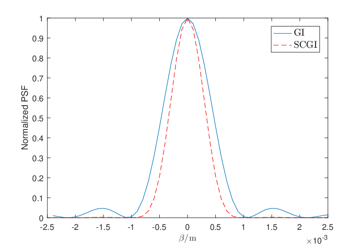
From Eq. (Second-order Cumulants Ghost Imaging), we find that $L(\beta)$ affects the resolution of SCGI. In order to understand how $L(\beta)$ affects the resolution, we study the case where the object is two-pinholes. The two pinholes are at $\alpha$ and $\alpha^{{}^{\prime}}=-\alpha$, respectively. The image of the object as shown in Fig. 3. From Fig. 3(a) and Fig. 3(b), we can find the image of the object when $L(\beta)=0$ is clear than it when $L(\beta)\neq 0$. This is because the cross-information which cannot be distinguished between $\kappa_{2}(\alpha,\beta)$ and $\kappa_{2}(\alpha^{{}^{\prime}},\beta)$ is generated when $\langle[\Delta G^{(2)}(I_{0},\alpha,\beta)-\langle\Delta G^{(2)}(I_{0},\alpha,\beta)\rangle][\Delta G^{(2)}(I_{0},\alpha^{{}^{\prime}},\beta)-\langle\Delta G^{(2)}(I_{0},\alpha^{{}^{\prime}},\beta)\rangle]\rangle\neq 0$.

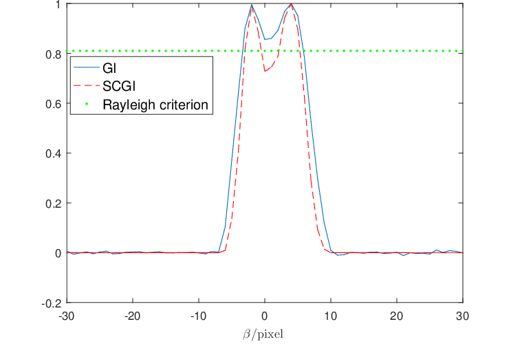
Compared with GI, the resolution of SCGI is better, when $L(\beta)\neq 0$. The detailed verification is as follows: We use the Rayleigh criterion to describe the resolution of the GIPaúr et al. 2016. Rayleigh criterion specifies the minimum separation between two incoherent point source ($\alpha_{o}$ and $\alpha_{o}^{{}^{\prime}}$. For simplification, we set $\alpha_{o}$=-$\alpha_{o}^{{}^{\prime}}$) that may be resolved into distinct objectPaúr et al. 2016. For the GI, because that the form of intensity PSF is $\text{sinc}^{2}$ function, so Rayleigh-distance set as $d_{1}=|\alpha_{o}-\alpha_{o}^{{}^{\prime}}|$ when $\frac{\Delta G^{(2)}(I_{0},0)}{\Delta G^{(2)}(I_{0},\alpha_{o})}\approx 0.81$. We can get the result is that $\frac{\kappa_{2}(0)}{\kappa_{2}(\alpha_{o})}=0.6561<0.81$ when $|\alpha_{o}-\alpha_{o}^{{}^{\prime}}|=d_{1}$ by Eq. (Second-order Cumulants Ghost Imaging), the results means SCGI can enhance the resolution limit of the conventional GI system.

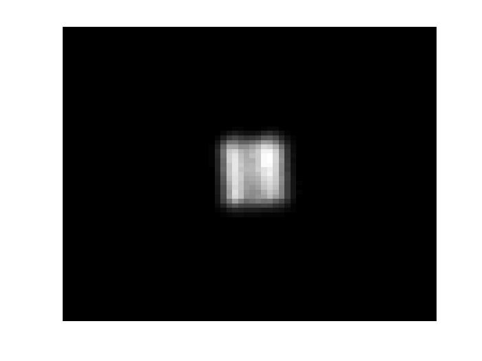
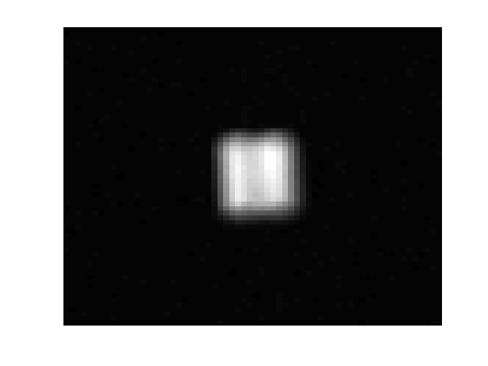
We verify our theoretical results via experiment. Our experimental setup is a conventional computational ghost imaging system, we used a projector as the light source. The diameter of light source is $3.3mm$ and the mean wavelength is $\lambda=550nm$. A double slit is taken as an object to measure the resolution of imaging. The slit width is $a_{1}=2\times 10^{-3}m$, slit center distance is $b_{1}=3\times 10^{-3}m$ and slit height is $g_{1}=8\times 10^{-3}m$. For simplification, we get different resolution image by manipulating $\Delta s$ ($\Delta s=s_{r}-s_{o}$) instead of $b_{1}$Zeng et al. 2017; Gatti, Magatti, and Ferri 2008; Ferri et al. 2008. We can get that $d_{1}\approx 2.3mm$ when $s_{o}=0.35m$ and $\Delta s=0.4m$, which is obvious smaller than $b_{1}$. When $\Delta s=0.85m$, $d_{1}\approx 3.1mm$ which is larger than $b_{1}$. Thus, in the experiment we set $s_{o}=0.35m$, $\Delta s$ as $0.4m$ and $0.85m$ respectively. Fig. 4 shows the experimental results of images reconstructed by GI and SCGI for different $\Delta s$, respectively.

When $\Delta s=0.4m$, the result of SCGI is shown in Fig. 4(a) and the result of GI is shown in Fig. 4(b). Fig. 4(a) and Fig. 4(b) are shown that the image of double slit by SCGI is more clear than that by GI. The normalized horizontal section of the experimental results of Fig. 4(a) and Fig. 4(b) are shown in Fig. 4(c). The result of Fig. 4(c) shows that $\frac{\kappa_{2}(0)}{\text{max}(\kappa_{2}(\beta))}<\frac{\Delta G^{(2)}(I_{0},0)}{\text{max}(\Delta G^{(2)}(I_{0},\beta))}$. When $\Delta s=0.85m$, Fig. 4(d-f) are shown that the image of double slit by SCGI is more clear than that by GI when $b_{1}<d_{1}$. Above results suggest that SCGI can enhance the resolution limit of GI system. Our analysis is that $\kappa_{2}(\beta)$ has more information than $\Delta G^{(2)}(I_{0},\beta)$.

In conclusion, $\Delta G^{(2)}(I_{0},\beta)$ is replaced by $\kappa_{2}(\beta)$ to obtain the image of object in GI system. We call this protocol as Second-order Cumulants ghost imaging (SCGI). Our theoretical analysis and experimental results show that the resolution limit of conventional GI can be enhanced by SCGI without changing the experimental setup of GI. $\kappa_{2}(\beta)$ is the fluctuation information of $\Delta G^{(2)}(I_{0},\beta)$, so the resolution can be further enhanced by SCGI to the super-resolution schemes, such as compressive sensing technique, low-pass spatial filter scheme and so on.

This work is supported by the Science & Technology Development Project of Jilin Province (No.YDZJ202101ZYTS030).

*

REFERENCES

- Pittman et al. (1995) T. B. Pittman, Y. Shih, D. Strekalov, and A. V. Sergienko, “Optical imaging by means of two-photon quantum entanglement,” Physical Review A 52, R3429 (1995).
- Gao et al. (2019) C. Gao, X. Wang, L. Gou, Y. Feng, H. Cai, Z. Wang, and Z. Yao, “Ghost imaging for an occluded object,” Laser Physics Letters 16, 065202 (2019).
- Gao et al. (2017) C. Gao, X. Wang, Z. Wang, Z. Li, G. Du, F. Chang, and Z. Yao, “Optimization of computational ghost imaging,” Physical Review A 96, 023838 (2017).
- Gatti et al. (2004) A. Gatti, E. Brambilla, M. Bache, and L. A. Lugiato, “Ghost imaging with thermal light: comparing entanglement and classicalcorrelation,” Physical review letters 93, 093602 (2004).
- Ribeiro et al. (1994) P. S. Ribeiro, S. Pádua, J. M. Da Silva, and G. Barbosa, “Controlling the degree of visibility of young’s fringes with photon coincidence measurements,” Physical Review A 49, 4176 (1994).
- Gatti, Brambilla, and Lugiato (2003) A. Gatti, E. Brambilla, and L. Lugiato, “Entangled imaging and wave-particle duality: from the microscopic to the macroscopic realm,” Physical review letters 90, 133603 (2003).
- Meyers, Deacon, and Shih (2008) R. Meyers, K. S. Deacon, and Y. Shih, “Ghost-imaging experiment by measuring reflected photons,” Physical Review A 77, 041801 (2008).
- Cheng and Han (2004) J. Cheng and S. Han, “Incoherent coincidence imaging and its applicability in x-ray diffraction,” Physical review letters 92, 093903 (2004).
- Abouraddy et al. (2001) A. F. Abouraddy, B. E. Saleh, A. V. Sergienko, and M. C. Teich, “Role of entanglement in two-photon imaging,” Physical review letters 87, 123602 (2001).
- Baleine, Dogariu, and Agarwal (2006) E. Baleine, A. Dogariu, and G. S. Agarwal, “Correlated imaging with shaped spatially partially coherent light,” Optics letters 31, 2124–2126 (2006).
- Bennink, Bentley, and Boyd (2002) R. S. Bennink, S. J. Bentley, and R. W. Boyd, ““two-photon” coincidence imaging with a classical source,” Physical review letters 89, 113601 (2002).
- Gong and Han (2012) W. Gong and S. Han, “Experimental investigation of the quality of lensless super-resolution ghost imaging via sparsity constraints,” Physics Letters A 376, 1519–1522 (2012).
- Cheng (2009) J. Cheng, “Ghost imaging through turbulent atmosphere,” Optics express 17, 7916–7921 (2009).
- Meyers, Deacon, and Shih (2011) R. E. Meyers, K. S. Deacon, and Y. Shih, “Turbulence-free ghost imaging,” Applied Physics Letters 98, 111115 (2011).
- Chen et al. (2017) X.-H. Chen, F.-H. Kong, Q. Fu, S.-Y. Meng, and L.-A. Wu, “Sub-rayleigh resolution ghost imaging by spatial low-pass filtering,” Optics letters 42, 5290–5293 (2017).
- Wang et al. (2019) Y. Wang, Y. Zhou, S. Wang, F. Wang, R. Liu, H. Gao, P. Zhang, and F. Li, “Enhancement of spatial resolution of ghost imaging via localizing and thresholding,” Chinese Physics B 28, 044202 (2019).
- Scully and Zubairy (1999) M. O. Scully and M. S. Zubairy, “Quantum optics,” (1999).
- Du, Gong, and Han (2012) J. Du, W. Gong, and S. Han, “The influence of sparsity property of images on ghost imaging with thermal light,” Optics letters 37, 1067–1069 (2012).
- Kuplicki and Chan (2016) K. Kuplicki and K. W. C. Chan, “High-order ghost imaging using non-rayleigh speckle sources,” Optics express 24, 26766–26776 (2016).
- Meng et al. (2018) S.-Y. Meng, Y.-H. Sha, Q. Fu, Q.-Q. Bao, W.-W. Shi, G.-D. Li, X.-H. Chen, and L.-A. Wu, “Super-resolution imaging by anticorrelation of optical intensities,” Optics letters 43, 4759–4762 (2018).
- Sprigg, Peng, and Shih (2016) J. Sprigg, T. Peng, and Y. Shih, “Super-resolution imaging using the spatial-frequency filtered intensity fluctuation correlation,” Scientific reports 6, 1–7 (2016).
- Li et al. (2019) F. Li, C. Altuzarra, T. Li, M. Scully, and G. Agarwal, “Beyond sub-rayleigh imaging via high order correlation of speckle illumination,” Journal of Optics 21, 115604 (2019).
- Zeng et al. (2017) X. Zeng, Y. Bai, X. Shi, Y. Gao, and X. Fu, “The influence of the positive and negative defocusing on lensless ghost imaging,” Optics Communications 382, 415–420 (2017).
- Ferri et al. (2005) F. Ferri, D. Magatti, A. Gatti, M. Bache, E. Brambilla, and L. A. Lugiato, “High-resolution ghost image and ghost diffraction experiments with thermal light,” Physical review letters 94, 183602 (2005).
- Zhang et al. (2009) P. Zhang, W. Gong, X. Shen, D. Huang, and S. Han, “Improving resolution by the second-order correlation of light fields,” Optics letters 34, 1222–1224 (2009).
- Paúr et al. (2016) M. Paúr, B. Stoklasa, Z. Hradil, L. L. Sánchez-Soto, and J. Rehacek, “Achieving the ultimate optical resolution,” Optica 3, 1144–1147 (2016).
- Gatti, Magatti, and Ferri (2008) A. Gatti, D. Magatti, and F. Ferri, “Three-dimensional coherence of light speckles: theory,” Physical Review A 78, 063806 (2008).
- Ferri et al. (2008) F. Ferri, D. Magatti, V. Sala, and A. Gatti, “Longitudinal coherence in thermal ghost imaging,” Applied Physics Letters 92, 261109 (2008).