marginparsep has been altered.
topmargin has been altered.
marginparwidth has been altered.
marginparpush has been altered.
The page layout violates the ICML style.
Please do not change the page layout, or include packages like geometry, savetrees, or fullpage, which change it for you.
We’re not able to reliably undo arbitrary changes to the style. Please remove the offending package(s), or layout-changing commands and try again.
TESDA: Transform Enabled Statistical Detection of Attacks in Deep Neural Networks
Chandramouli Amarnath 1 Aishwarya H. Balwani 1 Kwondo Ma 1 Abhijit Chatterjee 1
Submitted to the MLSys Conference, Santa Clara, CA, USA, 2022.
Abstract
Deep neural networks (DNNs) are now the de facto choice for computer vision tasks such as image classification. However, their complexity and “black box” nature often renders the systems they’re deployed in vulnerable to a range of security threats. Successfully identifying such threats, especially in safety-critical real-world applications is thus of utmost importance, but still very much an open problem. We present TESDA, a low-overhead, flexible, and statistically grounded method for online detection of attacks by exploiting the discrepancies they cause in the distributions of intermediate layer features of DNNs. Unlike most prior work, we require neither dedicated hardware to run in real-time, nor the presence of a Trojan trigger to detect discrepancies in behavior. We empirically establish our method’s usefulness and practicality across multiple architectures, datasets and diverse attacks, consistently achieving detection coverages of above 95% with operation count overheads as low as 1-2%.
1 Introduction
The increasing use of intelligent systems in safety-critical applications has led to the widespread use of third-party providers to build and train Deep Neural Network (DNN) models Ribeiro et al. 2015. This outsourcing, however, opens up the DNN to attack by malicious actors. These attacks can take the form of Neural Trojans or Adversarial Attacks; In the former, backdoors are inserted into a DNN through manipulation of training, weights or data to facilitate on-line alteration of DNN behavior Liu et al. 2020. In the latter, inputs to a clean, non-backdoored DNN are perturbed to alter its behavior on-line Xu et al. 2019. We propose an approach for the detection of both, Neural Trojans and Adversarial Attacks in image classification DNNs.
In a Neural Trojan, the attacker inserts a backdoor into the DNN, called a Trojan ‘trigger’ such that the DNN performs normally until a specific trigger mask is applied to the input image. The trigger mask produces a specific pattern on the resultant image, causing the DNN to misclassify to a target class. These triggers can be inserted through hardware, training data poisoning or alteration of the training process Liu et al. 2020. An example is shown in Figure 1.

Detection of Neural Trojans is difficult due to the DNN behaving nominally until presented with the trigger mask. Current research either (a) Reverse-engineers the trigger mask from a potentially infected model, typically using machine learning methods to find and patch backdoors inserted into the DNN Chen et al. 2019; Wang et al. 2019, (b) Identifies trigger mask patterns in the input to the DNN either through input perturbation Gao et al. 2019b or learning expected behavior to classify an attack Chou et al. 2018, (c) Evaluates the training process for abnormal parameter behavior indicative of a backdoor Gao et al. 2019a; Baracaldo et al. 2018, or (d) Provides runtime detection by analyzing latent features extracted by the DNN and detecting outliers in the error of an image reconstructed from those features with respect to the input Javaheripi et al. 2020.
Methods of type (a) require the DNN to be taken offline for analysis so that time-consuming machine learning methods can be applied. Methods of type (b) incur high overhead since a compute intensive detector and DNN need to be run in sequence. Methods of type (c) require the defender to be able to oversee the entire training process and cannot simply be used post-training. Methods of type (d) incur high overhead due to utilization of algorithms Pati et al. 1993 that cannot be parallelized, thus requiring dedicated hardware for runtime protection. Further, none of the above methods have been tested for adversarial attack detection, and are unlikely to be able to detect adversarial attacks in the absence of trigger mask patterns.
In an Adversarial Attack or Adversarial Example, the attacker perturbs the inputs to the DNN to force misclassification without inserting a backdoor. In this case, the adversarial attacks are considered to be untargeted, aiming to force an erroneous output to any incorrect class. Adversarial attacks typically perturb the image just enough to force a misclassification. These attacks can be generated as an optimization problem of finding the minimally distorted image that forces misclassification Xu et al. 2019.
Defenses against adversarial attacks on DNNs involve (a) Adversarial training, in which attacked images are used to train the DNN Madry et al. 2019; Zhang et al. 2019, (b) Masking the gradient used by an iterative solver to generate the minimally distorted image that forces misclassification Carlini & Wagner 2017, (c) Establishing certificates for DNN resilience to adversarial attacks through computation of upper bounds for DNN loss and modifying training to minimize them Raghunathan et al. 2018, and (d) Detect adversarial inputs prior to prediction and discard those predictions Grosse et al. 2017. All of (a), (b) and (c) require alteration of the training itself and thus cannot provide out-of-the-box runtime attack detection. Methods in (d) provide runtime attack detection, but have yet to be tested on Neural Trojans and can often require high-overhead machine learning methods to process the input.
We therefore present Transform Enabled Statistical Detection of Attacks (TESDA), a detection method for both Neural Trojans and Adversarial Attacks in image classification DNNs, via the extraction of pertinent features at specified intermediate layers of the DNN. In contrast to prior art, the key contributions of our work are:
(1) A low-overhead, high-coverage real-time detection method for security attacks in DNNs, with detection coverage of up to 99% whilst incurring operation count overheads of only 1-2%.
(2) A flexible method for the detection of both Neural Trojans and Adversarial Attacks that does not rely on static Trojan trigger mask patterns for detection.
(3) Theoretically guided hyperparameter tuning that enables control of false positive and negative detection rates.
(4) An easy setup, requiring only a sampling of DNN intermediate layer outputs on training data pre-deployment.
| Defense Mechanism | On-Line Capabilities | Overhead | Tested On |
| ||||||||
| CleaNN |
|
|
|
Yes | ||||||||
| STRIP | Detection | Very High |
|
Yes | ||||||||
| Neural Cleanse |
|
Very High |
|
| ||||||||
| TESDA | Detection |
|
|
Not Necessary |
The paper is organized as follows: Section 2 discusses prior art, contrasting our choice of test case attacks and assumptions versus those of previous methods. Sections 3, 4, 5 present an overview of our proposed approach, its detailed description, and our experimental results on commonly used DNNs and datasets respectively. Sections 6, 7 end with a discussion of some ablation studies and conclusions.
2 Background
2.1 Threat Models and Approach Assumptions
The three attacks tested here are discussed below. An overview of the assumptions made by the proposed detector is then compared qualitatively against prior art.
(1) Targeted Bit Trojan: The Targeted Bit Trojan (TBT) attack Rakin et al. 2019 creates DNN backdoors via bitflips made in layer weights stored in memory. The trigger mask is a static pattern. The attack is inserted after DNN deployment. The attacker is assumed to have access to a subset of training data and a copy of the trained model to build the Trojan and to insert it via bitflips in weights.
(2) Input-Aware Backdoor Attack: In this attack Nguyen & Tran 2020 the DNN a backdoor is inserted during training such that the DNN misclassifies to a target class when presented with the trigger mask. This attack is different from prior art due to its use of a dynamic trigger mask as a function of the input. The attacker is assumed to have control of the training process, shipping a contaminated DNN around which our proposed detector will be built.
(3) Projected Gradient Descent (PGD) Attack: The attacker is assumed to have information about the trained model and its gradients to compute the input perturbations to force DNN misclassification to any class Madry et al. 2019. The PGD attack accomplishes this by attempting to find the input perturbations that maximize DNN loss while keeping perturbation size smaller than a predefined bound.
In contrast to prior art, the proposed detector is built around a trained DNN model and requires access to the trained DNN’s intermediate layer outputs on clean training data to be able to profile the DNN. The detector can be built on a clean or contaminated model, does not require DNN re-training and is not tailored to specific attacks.
2.2 Comparison to Prior Art
A qualitative comparison of the proposed approach against prior art is provided in Table 1. We compare against CleaNN Javaheripi et al. 2020, STRIP Gao et al. 2019b and Neural Cleanse Wang et al. 2019. STRIP provides on-line detection of Neural Trojans but incurs very high overhead due to the need to repeatedly perturb inputs to detect a Trojan trigger. CleaNN provides real-time detection and defense against Trojan triggers via dedicated FPGA hardware acceleration but has high overhead without that hardware. Neural Cleanse uses machine learning methods to find and patch backdoors in a DNN and does not provide real time attack detection. In contrast to this, TESDA provides low-overhead real-time attack detection with operation count overheads of 1-2% before acceleration or optimization and does not require dedicated hardware. TESDA does not use iterative methods leveraged by prior art such as OMP Pati et al. 1993, thereby enabling future parallelization.
All other approaches in Table 1 have been tested by their authors against BadNets Gu et al. 2017, an attack which inserts Trojan backdoors during training. Neural Cleanse and STRIP are also tested by their authors against a backdoor Trojaning Attack Liu et al. 2018a. CleaNN is also tested by its authors against the backdoor attack of TrojanNN Liu et al. 2018b. By contrast, our approach is verified on the input-aware dynamic backdoor attack Nguyen & Tran 2020, which has been shown to break STRIP and Neural Cleanse using input-specific trigger masks. TESDA is also verified on the Targeted Bit Trojan Rakin et al. 2019, which is inserted after training, bypassing offline defenses. The greater flexibility of TESDA is verified by tests on the Projected Gradient Descent adversarial attack Madry et al. 2019. Our approach does not require static trigger mask patterns to detect an attack.
3 Approach Overview
3.1 Network-Level Detector Deployment

Figure 2 shows the deployment of TESDA on a DNN. Each layer’s output is reduced to a feature coefficient in the dimensionality reduction and feature extraction blocks. These blocks employ identical methods for each layer and are discussed further in the following subsection. For a network of layers this yields an length vector of s, in Block 1. A multidimensional distribution is fitted to the set of s across the DNN training data to enable attack detection (Block 2a). If the produced during operation is an outlier with respect to that distribution (Block 2b), it is considered indicative of an attack.
3.2 Detector Components: Single Layer

Figure 3 shows the process of attack detection applied to a single convolutional layer of kernels. After convolution, bias addition and activation, each kernel produces a 2D image, giving a layer output of an such images, a 3D tensor. The size of this tensor can make direct analysis expensive. The first step is to reduce this to low dimensional features. This is done in blocks 2-4 of Figure 3, which takes the layer output from Block 1b.
The first step in feature extraction and dimensionality reduction is reduction of each kernel output to its frequency coefficients using the Discrete Cosine Transform (DCT) Oppenheim & Schafer 2009 (Block 2). This gives an -length transformed tensor where each element is a 2D array of DCT frequency coefficients. One or more of the DCT coefficients from each transformed kernel output may be chosen for further analysis. In Block 3 of Figure 3, DCT coefficients were chosen from each element of the tensor, giving an array of DCT coefficients.
In Block 4, a Principal Components Analysis (PCA) Shlens 2014 transformation is applied to each of the frequency coefficients in the -length array obtained from Block-3. The PCA is fit to each row of the set of chosen DCT coefficients from the layer outputs across the training data set. This yields an array of projections, with coefficients ordered according to significance. Each is a vector of the th PCA coefficients of all DCT coefficients chosen. One or more s can be chosen from for attack detection in Blocks 4a and 4b. For a dense layer, a PCA is taken along the layer output vector directly and a subset of can be used for attack detection.
Attack detection is done based on the distribution of the chosen subset of , . If the from Block-4 is an outlier with respect to its distribution over training data, an attack is indicated. A multivariate distribution is fitted to the values on the training data in Block 4a. This distribution is used to set thresholds for outlier detection post-deployment of the DNN and detector. Statistical tests leveraging the training distribution for outlier detection are used here, allowing threshold adjustment to ensure a desired false positive rate.
4 Approach Details
4.1 Feature Extraction and Dimensionality Reduction
In Blocks 2-4 of Figure 3 the output tensor of each convolutional layer under examination is reduced to a set of PCA coefficients that represents layer behavior. This begins with the Discrete Cosine Transform of Block-2 to extract the frequency components of each convolution kernel output.
4.1.1 DCT Analysis
Each convolution kernel in each layer under analysis outputs an image after activation. The DCT Oppenheim & Schafer 2009 is taken on the output of each kernel to reduce these images to frequency components in the form of a sequence of sinusoids (cosines) in two dimensions oscillating. A set of frequency components is chosen for further analysis. The same components are chosen across all transformed kernel outputs. This yields a matrix of the chosen DCT coefficients for the th layer in the network. While Trojan trigger presence has been seen to typically affect higher frequency coefficients Javaheripi et al. 2020, the flow in Figure 3 also targets adversarial attacks. A range of DCT coefficients is thus tested in this work. In our experiments we predominantly use . Further experiments using are detailed in Appendix E.
4.1.2 Principal Component Analysis
For a network of layers, the process above yields a set where each is a matrix of DCT coefficients. We further reduce the dimensionality of this set using Principal Component Analysis (PCA) Shlens 2014, by applying it independently to each .
The PCA transforms each row of to a vector space whose basis vectors are orthogonal to one another. The elements of each row of the transformed matrix are ordered according to the energy in each principal component (or basis vector of the transform space), providing an optimal decomposition of each row of . As a linear transformation, the PCA has low overhead. The transformation matrices for the th layer are obtained from the mean and covariance of the rows of the set of produced across the training data set.

The vector of DCT coefficients is thus transformed into a matrix for each layer , such that each column of , is a vector of the th PCA coefficients of all DCT coefficients chosen. For a dense layer the DCT decomposition is not required and the PCA transform is taken from the output vector of the dense layer for each input to the DNN. The PCA for a dense layer is fitted to the set of outputs produced for each input in the training data set.
One or more columns can then be taken from each for the purposes of outlier detection, reducing the high-dimensional tensor output from a convolutional layer to just a vector containing few coefficients. We note however that the higher energy coefficients (e.g., ) are seen to contain lesser information about the outliers, i.e., perform worse at outlier detection (Figure 4) than their lower energy counterparts (e.g., ). We therefore restrict ourselves to using just the lowest energy coefficient corresponding to each layer, giving us a vector for every sample, where
4.2 Attack Detection with Elliptic Envelopes
To detect an attack we check if the obtained for a particular sample is an outlier with respect to the true (i.e., clean) distribution of as observed in the training set. This of course would only work if an attack appreciably alters the distribution of the used in construction of the vector , which we do confirm empirically to hold true (Figure 5).

We then approximate the distribution of the clean across the training set as a multidimensional Gaussian , allowing us to leverage the statistical tools available for robust Gaussian parameter estimation and model fitting. Specifically, we use the minimum covariance determinant (MCD) method Rousseeuw 1984; Rousseeuw 1985; Rousseeuw & Driessen 1999 which given a training set with -dimensional samples of which at most are outliers, finds estimates for the true mean and covariance. To do so MCD finds samples from the training set whose covariance matrix has the least determinant and fits a Gaussian to them, implicitly making the assumption that Subsequently, any sample that is outside the Elliptic Envelope described by , i.e., has a Mahalanobis distance , a pre-specified threshold, is classified as an outlier. It should be noted that for Gaussian models the MCD method has been shown to be asymptotically consistent Butler et al. 1993, i.e., as . An example of the MCD based elliptic envelope fit to noisy data processed through a DNN is shown in Figure 6.

4.2.1 Hyperparameter Tuning to Match Target False Positive and False Negative Rates
Due to its simplicity and interpretability, the MCD method lends itself to principled hyperparameter tuning which allows us to choose the offset such that given an approximate upper bound on the degree of contamination of the training data, , we can stay under either a target false negative (FNR) or false positive rate (FPR).
Let be the robust sample mean and covariance estimates provided by the MCD method. Further assume and For a sample to be classified as an outlier (i.e., an attack) we require that , or equivalently , where is the squared Mahalanobis distance of and is a constant computed over and fit to the entire training data. Specifically, depends on the contamination parameter and is fit on the training data such that the number of outliers .
Given that acts as an upper bound on the contamination of the training set, we want to pick such that . At the same time, by the multivariate Chebyshev inequality Stellato et al. 2017 we have . Equating the two, we get .
Provided an expression for we have a principled way of choosing the contamination parameter so as to stay under a specified false negative () or false positive () rate.
False negative rate: The FNR is by definition the complement of the true positive rate, which on the training set must be . Therefore to minimize FNR, we set and then fix .
False positive rate: To minimize false positives we simply require that for clean samples . We therefore set and fix
Additional details regarding the derivation of the expression for are provided in Appendix A.
4.2.2 Deriving Tighter Bounds for Outlier Detection
Leveraging the fact that the distribution of for clean is given by the chi-squared distribution with degrees of freedom, i.e., (Appendix B), it is possible to have bounds tighter than those using Chebyshev’s inequality, with the caveats that i) the expression for would have to be split into multiple expressions depending on its range, or ii) the dependence of on might no longer be expressible as closed form expressions of elementary functions.
For example, noting that the distribution is sub-exponential with parameters Ghosh 2021, one can write the corresponding sub-exponential tail bound Wainwright 2019, resulting in the following expressions
Alternatively, one could also write a Chernoff bound Wainwright 2019 that yields , being the Lambert W function Bronstein et al. 2008 whose values may be calculated numerically.
4.3 The TESDA Algorithm
We consolidate and present the complete detection process in Algorithm 1. TESDA begins by taking as input the layer wise outputs from the network (Line 1) of a DNN that produces a label for an input . It then initializes the array for the input to the outlier detector (Line 2) and calls the processing loop (Line 3) that runs for each of the layers. In the loop, first, DCT is applied to the outputs of each kernel of the th convolutional layer and DCT-Analyzer() returns the matrix of selected DCT coefficients (Line 4). In case of a dense layer, the DCT step is skipped and the function simply returns the vector of layer outputs. Next, the rows of over the entire training data are transformed using PCA (Line 5) to produce a matrix of PCA coefficients, where every row of corresponds to a layer of the DNN and every column corresponds to a PC. Starting with the last one, columns of are assigned as features of the vector (Line 6) and the complete is fed to Elliptic-Envelope, i.e., the outlier detector (Line 8). If is classified as an outlier, we flag it as an attack on the network. We empirically validate TESDA on a variety of test cases, the results of which are presented in Section 5.
5 Experimental Results
5.1 Experimental Metrics
We evaluate TESDA using the following metrics:
Detection Coverage: Detection coverage is the number of detected attacks divided by the total number of attacks. This is the true positive rate of the attack detection system.
False Positive Rate (FPR): This is the percentage of time that the detector flags clean operation, obtained by running the network and detector across clean test data.
F1-Score: The F1-score is the harmonic mean of precision and recall. Precision is the true positive rate divided by the sum of true and false positive rates. Recall is the true positive rate divided by the sum of true positive and negative rate. This is represented as a percentage value from 0-100%.
Algorithm overhead for the attack detector is calculated using CPU performance counter data and measured relative to the resources consumed by the DNN run on the CPU. Further details are provided in Section 5.6.
5.2 Network, Dataset and Ablation Details
The datasets used here are CIFAR-10 Krizhevsky 2009 and GTSRB Houben et al. 2013. CIFAR-10 consists of 32x32 color images, with 50K training and 10K test images across 10 classes. GTSRB consists of 43 traffic sign classes across a training set of 39209 labeled images and 12630 test images. Tests were conducted on these for two DNNs.
The first network tested is ResNet-18 He et al. 2015 using the CIFAR-10 dataset. It has one input convolutional layer, four residual blocks, one average pooling and one output linear layer. In each residual block an identity mapping combines its input with the result of a convolution ‘branch’ for ReLu activation. The second network examined is PreAct ResNet-18 He et al. 2016 using the GTSRB dataset. For PreAct ResNet, the ‘branch’ is identical to ResNet-18, with one ReLu moved from the end of the unit to the start of the branch. PreAct ResNet-18 has one convolutional input layer, four residual blocks, one average pooling layer and one output linear layer. The detector for both networks conducts feature extraction with and selects the final from the PCA matrix at each residual block for detection.
Ablation Test Cases: The performance of the system is tested for (1) Different outlier thresholds with the detector concurrently connected across all residual blocks and the final layer for ResNet-18 and PreAct ResNet-18 and (2) For each residual block and the final layer with the detector connected to them individually. Metrics are recorded as per Section 5.1. For relevant test cases we also record (3) The effects of using different single DCT coefficients.
5.3 Targeted Bit Trojan
The Targeted Bit Trojan (TBT) attack Rakin et al. 2019 creates backdoors in a DNN, forcing misclassification when presented with the trigger mask via bitflips made in layer weights stored in memory. The attack was generated by modifying code provided by the authors.
The attack works as follows: (a) In the Insertion step, alterations to specific weight bits are made to map the input to a specific target class in the presence of the trigger. The trigger is designed to force vulnerable neurons in the target layer linked to the target class to fire at a large value. The TBT flips vulnerable layer weight bits in memory such that the DNN performs nominally without the trigger. It is shown in Rakin et al. 2019 that only 84 bit flips out of 88 million bits are needed to classify 92% of images to a target class on Resnet-18 for CIFAR10. Since these weights are stored in memory, row-hammer attacks Kim et al. 2014 can be used for insertion. (b) In the triggering step of the attack, the image trigger (mask) is inserted into the DNN input image. The mask modifies pixel values in a small area of the image and causes mis-classification by the DNN to an incorrect target class, as in Figure 1. The TBT is thus inserted after deployment of the DNN. This bypasses pre-deployment scans. The TBT here attacks the final layer of ResNet-18, forcing misclassification to target class 2 (Bird).
TESDA is tested for the TBT using a pretrained ResNet-18 trained on CIFAR-10 provided by the authors for cases (1) and (2) from Section 5.2. Since the TBT only attacks the final linear layer, there are no material changes to convolutional layers and case (3) is not evaluated (the DCT is taken only for convolutional layers).

(1) Detector performance for different levels of outlier threshold is shown in Figure 7. By varying , the level of false positives seen in the detector can be adjusted. For all outlier thresholds, detection coverage remains above 99% and varies only marginally, while F1-score falls as the threshold rises. Italicized figures are data point values for F1-score and non-italicized ones are for coverage.

(2) Detector performance for each residual block and the final layer is shown in Figure 8. The detector is connected across each unit and the final layer alone. Clean and Trojaned data are run across the detector. The F1-score is negligible until the final layer, which is the one targeted by the TBT. Here the F1-score and the coverage remain above 99%. used here was 0.01.
5.4 Input-Aware Dynamic Backdoor Attack
The second attack tested is the Input-Aware Dynamic Backdoor Attack applied to PreAct ResNet-18 on GTSRB using code provided by the authors Nguyen & Tran 2020. In this attack, a backdoor is inserted during DNN training to force misclassification to a target class when presented with the trigger pattern. This attack differs from prior benchmarks in its use of an input-aware dynamic trigger mask. The trigger pattern generated in training is a function of the input image, dictated by an autoencoder. Training is modified to ensure the triggers are usable only for the image they are intended for. These dynamic triggers have been shown to bypass defenses such as STRIP. The attack has more than 99% effectiveness on GTSRB. The trained DNN is already contaminated when run on clean training data to set up the detector. The detector set up based on the training set generated by this contaminated network is used to detect the attack when a trigger mask is passed. The defender is assumed to be able to run the contaminated DNN on clean training data before deployment. The attack here forces misclassification to target class 0 (20kph speed limit sign).
The detector performance for this attack is tested on PreAct ResNet-18 for cases 1-3 of Section 5.2.


(1) Detector performance for different levels of outlier detection threshold is shown in Figure 9. The italicized figures are the data point values for F1-score and the non-italicized ones are for the coverage. The F1-score peaks at or a 0.4% expected false positive rate. This gives a coverage of 97.08% and an FPR of 1.95%. A threshold of yields a coverage of 98.4% and a false positive rate of 3.8%.
(2) Detector performance for each residual block is shown in Figure 10. The backdoor attack affects each layer of the DNN when executed, and that effect is seen here with coverage being materially significant at each layer. Coverage is highest at residual block 1 and the final layer (76.9% and 57.2% respectively), for the outlier threshold of 0.01.

(3) Detector performance for different DCT coefficients selected for the PCA is shown in Figure 11. Since here, changing the DCT coefficient affects performance. The italicized figures are the data point values for F1-score and the non-italicized ones are for the coverage. The DCT coefficient number is displayed along with its (X,Y) indices in the transformed image. The coverage drops sharply after the first DCT coefficient, with local peaks every fourth DCT coefficient (1, 4 and 8). The F1-score remains high due to the low false positive rate, but shows a similar trend.
5.5 Adversarial Attack: Projected Gradient Descent
The third attack tested is the Projected Gradient Descent (PGD) adversarial attack Madry et al. 2019. The attacker is assumed to have information about the model gradients to compute the required input perturbations for the DNN to force a misclassification to any class. The PGD attack accomplishes this by attempting to find the input perturbations that maximize model loss while keeping perturbations smaller than an amount , measured as the norm of the difference between the clean input and perturbed input. This is done via a gradient descent taking steps in the direction of maximum loss, projecting the resultant perturbation back into the space around the clean input and iterating further. This is implemented for the clean CIFAR-10 ResNet-18 model used for the TBT attack via the Cleverhans v4.0.0 Papernot et al. 2018 adversarial benchmarking library. The value of of the PGD used here is 0.3. The attack forces misclassification with more than 99% effectiveness for ResNet-18 on CIFAR-10.
The detector performance against the PGD attack is tested on ResNet-18 for cases 1-3 of Section 5.2.

(1) Detector performance for different levels of outlier detection thresholds is shown in Figure 12. The F1-score peaks at . This gives a coverage of 95.73% and a false positive rate of 4.35%. yields a coverage of 94.16% and a false positive rate of 3.1%. The italicized figures are the data point values for F1-score and the non-italicized ones are for the coverage.

(2) Detector performance for each residual block is shown in Figure 10. The backdoor attack is not targeted at any one layer, thus coverage is significant at each layer. Coverage is highest at residual block 2 (76.9% and a 2.98% false positive Rate), for the outlier threshold of 0.03.

(3) Detector performance for different DCT coefficients selected for the PCA is shown in Figure 14. The italicized figures are the data point values for F1-score and the non-italicized ones are for the coverage. The DCT coefficient number is displayed along with its (X,Y) indices in the transformed image. The coverage and F1-score drop sharply after the first DCT coefficient.
5.6 Algorithm Overhead
| Metric |
|
| |||||
|---|---|---|---|---|---|---|---|
|
1.31 | 1.13 | |||||
|
19.17 | 16.02 | |||||
|
175.8 | 117.8 | |||||
|
1.478 | 0.92 |
The performance overhead of TESDA relative to the DNN when connected across all residual blocks and the final linear layer is shown in Table 2. PreAct ResNet-18 uses the trained model provided by the authors of Nguyen & Tran 2020. ResNet-18 uses the trained model provided by the authors of Rakin et al. 2019. Overhead was calculated using the Performance Application Programming Interface library Terpstra et al., which allows access to CPU counters. The average overhead was calculated across the test data of GTSRB for PreAct ResNet-18 and CIFAR-10 for ResNet-18. The DNNs were written in PyTorch Paszke et al. 2019. The detector used Scikit-Learn Buitinck et al. 2013. This was run on an Intel Xeon W-2123 CPU. The counters were run for the DNN across DNN inference alone. The counters for the detector were run across conversion of intermediate layer data to suitable formats, feature extraction and outlier detection on the extracted .
The overhead is ultra-low for floating point operations, at around 1%. Vector operations are still very low at less than 20% overhead. Since the detector does not write much to cache and reads a great deal from the cache (layer outputs for analysis), the cache write overhead is extremely low (0.8-1.2%). The cache read overhead is high compared to the DNN, which does not read much data from the CPU cache. The detector has low overhead without requiring dedicated hardware, run using common libraries on a general purpose CPU. Overhead can be reduced by reducing the number of layers the detector takes inputs from concurrently.
6 Ablation Studies and Discussion
6.1 Threshold Variation
As expected, increasing the outlier threshold (Figures 7, 9 and 12) increases detection and false positive rate. Assuming a general detection scenario with the detector built pre-deployment, this would give coverages of 91.69% on PGD attacks and 99% on TBT for a false positive rate of 1.99% for ResNet-18 on CIFAR-10 with at 0.02. The TBT is seen to achieve near-total detection coverage at very low thresholds, indicative of the drastic change in behavior in the final (targeted) layer caused by the attack. More subtle attacks like the input-aware backdoor and PGD are less extreme and therefore have lower coverage at low thresholds.
6.2 Layer Ablations
Each of the attacks tested shows different behavior with the detector restricted to one layer (Figures 8, 10 and 13). The TBT attacks the final layer weights and thus shows high coverage in that layer alone. The input-aware backdoor attack shows high coverage across the output of Residual Block 1 and the final layer, likely due to the trigger patterns changing the behavior of Residual Block 1 more than succeeding units. The final layer behavior changes due to earlier layers being affected by the attack. The PGD attack is most easily detected at the output of Residual Block 2 ( coverage). This residual block can be considered the diverging point Cantareira et al. 2021 where the adversarial attack forces misclassification. From the experimental results, it can be seen that Residual Blocks 3 and 4 are of lower significance for all considered attacks. The lightest possible detector configuration for these attacks would thus be connected across Residual Blocks 1, 2 and the final layer.
6.3 DCT Coefficient Variation
Variation of DCT coefficients chosen from each convolutional layer’s output to check effect on detection was done for the input-aware backdoor attack on PreAct ResNet-18 and the PGD attack on ResNet-18 (Figures 11 and 14). For the input-aware backdoor attack, detection remains materially significant across a range of DCT coefficients’ final values. The backdoor’s alteration of the features extracted by the DNN thus affects a range of frequencies. For the PGD attack, the constraint to limit the deviation in the image based on the norm of the perturbation seems to limit the effect of the PGD attack on higher frequencies. It instead appears to add perturbations that shift the final PCA coefficient of the first (DC) DCT coefficient. The use of more than one DCT coefficient has little impact on detection, marginally raising coverage for the input-aware backdoor. Further details can be found in Appendix E.
7 Conclusion
Our work presents and validates TESDA, a scheme for DNN security attack detection on two different types of state of the art attacks. We find that it is extremely comparable in terms of performance to strong baselines from prior art, while operating at a much lower hardware overhead and working for a broader range of attacks. The extension of TESDA to online defense along with further study of its real, in-field performance is envisioned as future work.
Acknowledgements
This research was supported by the Semiconductor Research Corporation under Auto Task 2892.001 and in part by the U.S. National Science Foundation under Grant S&AS:1723997.
References
- Baracaldo et al. (2018) Baracaldo, N., Chen, B., Ludwig, H., Safavi, A., and Zhang, R. Detecting poisoning attacks on machine learning in iot environments. 09 2018. doi: 10.1109/ICIOT.2018.00015.
- Bronstein et al. (2008) Bronstein, M., Corless, R. M., Davenport, J. H., and Jeffrey, D. J. Algebraic properties of the lambert w function from a result of rosenlicht and of liouville. Integral Transforms and Special Functions, 19(10):709–712, 2008.
- Buitinck et al. (2013) Buitinck, L., Louppe, G., Blondel, M., Pedregosa, F., Mueller, A., Grisel, O., Niculae, V., Prettenhofer, P., Gramfort, A., Grobler, J., Layton, R., VanderPlas, J., Joly, A., Holt, B., and Varoquaux, G. API design for machine learning software: experiences from the scikit-learn project. In ECML PKDD Workshop: Languages for Data Mining and Machine Learning, pp. 108–122, 2013.
- Butler et al. (1993) Butler, R., Davies, P., and Jhun, M. Asymptotics for the minimum covariance determinant estimator. The Annals of Statistics, pp. 1385–1400, 1993.
- Cantareira et al. (2021) Cantareira, G. D., Mello, R. F., and Paulovich, F. V. Explainable adversarial attacks in deep neural networks using activation profiles. CoRR, abs/2103.10229, 2021. URL https://arxiv.org/abs/2103.10229.
- Carlini & Wagner (2017) Carlini, N. and Wagner, D. Towards evaluating the robustness of neural networks. In 2017 IEEE Symposium on Security and Privacy (SP), pp. 39–57, 2017. doi: 10.1109/SP.2017.49.
- Chen et al. (2019) Chen, H., Fu, C., Zhao, J., and Koushanfar, F. Deepinspect: A black-box trojan detection and mitigation framework for deep neural networks. pp. 4658–4664, 08 2019. doi: 10.24963/ijcai.2019/647.
- Chou et al. (2018) Chou, E., Tramèr, F., Pellegrino, G., and Boneh, D. Sentinet: Detecting physical attacks against deep learning systems. CoRR, abs/1812.00292, 2018. URL http://arxiv.org/abs/1812.00292.
- Gao et al. (2019a) Gao, H., Yunfang, C., and Zhang, W. Detection of trojaning attack on neural networks via cost of sample classification. Security and Communication Networks, 2019:1–12, 11 2019a. doi: 10.1155/2019/1953839.
- Gao et al. (2019b) Gao, Y., Xu, C., Wang, D., Chen, S., Ranasinghe, D. C., and Nepal, S. STRIP: A defence against trojan attacks on deep neural networks. CoRR, abs/1902.06531, 2019b. URL http://arxiv.org/abs/1902.06531.
- Ghosh (2021) Ghosh, M. Exponential tail bounds for chisquared random variables. Journal of Statistical Theory and Practice, 15(2):1–6, 2021.
- Grosse et al. (2017) Grosse, K., Manoharan, P., Papernot, N., Backes, M., and Mcdaniel, P. On the (statistical) detection of adversarial examples. ArXiv, abs/1702.06280, 2017.
- Gu et al. (2017) Gu, T., Dolan-Gavitt, B., and Garg, S. Badnets: Identifying vulnerabilities in the machine learning model supply chain. CoRR, abs/1708.06733, 2017. URL http://arxiv.org/abs/1708.06733.
- He et al. (2015) He, K., Zhang, X., Ren, S., and Sun, J. Deep residual learning for image recognition. CoRR, abs/1512.03385, 2015. URL http://arxiv.org/abs/1512.03385.
- He et al. (2016) He, K., Zhang, X., Ren, S., and Sun, J. Identity mappings in deep residual networks. CoRR, abs/1603.05027, 2016. URL http://arxiv.org/abs/1603.05027.
- Houben et al. (2013) Houben, S., Stallkamp, J., Salmen, J., Schlipsing, M., and Igel, C. Detection of traffic signs in real-world images: The German Traffic Sign Detection Benchmark. In International Joint Conference on Neural Networks, number 1288, 2013.
- Javaheripi et al. (2020) Javaheripi, M., Samragh, M., Fields, G., Javidi, T., and Koushanfar, F. CLEANN: accelerated trojan shield for embedded neural networks. CoRR, abs/2009.02326, 2020. URL https://arxiv.org/abs/2009.02326.
- Kim et al. (2014) Kim, Y., Daly, R., Kim, J., Fallin, C., Lee, J. H., Lee, D., Wilkerson, C., Lai, K., and Mutlu, O. Flipping bits in memory without accessing them: An experimental study of dram disturbance errors. SIGARCH Comput. Archit. News, 42(3):361–372, June 2014. ISSN 0163-5964. doi: 10.1145/2678373.2665726. URL https://doi.org/10.1145/2678373.2665726.
- Krizhevsky (2009) Krizhevsky, A. Learning multiple layers of features from tiny images. Technical report, 2009.
- Liu et al. (2018a) Liu, Y., Ma, S., Aafer, Y., Lee, W.-C., Zhai, J., Wang, W., and Zhang, X. Trojaning attack on neural networks. In NDSS, 2018a.
- Liu et al. (2018b) Liu, Y., Ma, S., Aafer, Y., Lee, W.-C., Zhai, J., Wang, W., and Zhang, X. Trojaning attack on neural networks. In 25nd Annual Network and Distributed System Security Symposium, NDSS 2018, San Diego, California, USA, February 18-221, 2018. The Internet Society, 2018b.
- Liu et al. (2020) Liu, Y., Mondal, A., Chakraborty, A., Zuzak, M., Jacobsen, N., Xing, D., and Srivastava, A. A survey on neural trojans. In 2020 21st International Symposium on Quality Electronic Design (ISQED), pp. 33–39, 2020. doi: 10.1109/ISQED48828.2020.9137011.
- Madry et al. (2019) Madry, A., Makelov, A., Schmidt, L., Tsipras, D., and Vladu, A. Towards deep learning models resistant to adversarial attacks, 2019.
- Nguyen & Tran (2020) Nguyen, A. and Tran, A. Input-aware dynamic backdoor attack. CoRR, abs/2010.08138, 2020. URL https://arxiv.org/abs/2010.08138.
- Oppenheim & Schafer (2009) Oppenheim, A. V. and Schafer, R. W. Discrete-Time Signal Processing. Prentice Hall Press, USA, 3rd edition, 2009. ISBN 0131988425.
- Papernot et al. (2018) Papernot, N., Faghri, F., Carlini, N., Goodfellow, I., Feinman, R., Kurakin, A., Xie, C., Sharma, Y., Brown, T., Roy, A., Matyasko, A., Behzadan, V., Hambardzumyan, K., Zhang, Z., Juang, Y.-L., Li, Z., Sheatsley, R., Garg, A., Uesato, J., Gierke, W., Dong, Y., Berthelot, D., Hendricks, P., Rauber, J., and Long, R. Technical report on the cleverhans v2.1.0 adversarial examples library. arXiv preprint arXiv:1610.00768, 2018.
- Paszke et al. (2019) Paszke, A., Gross, S., Massa, F., Lerer, A., Bradbury, J., Chanan, G., Killeen, T., Lin, Z., Gimelshein, N., Antiga, L., Desmaison, A., Kopf, A., Yang, E., DeVito, Z., Raison, M., Tejani, A., Chilamkurthy, S., Steiner, B., Fang, L., Bai, J., and Chintala, S. Pytorch: An imperative style, high-performance deep learning library. In Wallach, H., Larochelle, H., Beygelzimer, A., d'Alché-Buc, F., Fox, E., and Garnett, R. (eds.), Advances in Neural Information Processing Systems 32, pp. 8024–8035. Curran Associates, Inc., 2019.
- Pati et al. (1993) Pati, Y. C., Rezaiifar, R., and Krishnaprasad, P. S. Orthogonal matching pursuit: Recursive function approximation with applications to wavelet decomposition. In in Conference Record of The Twenty-Seventh Asilomar Conference on Signals, Systems and Computers, pp. 1–3, 1993.
- Raghunathan et al. (2018) Raghunathan, A., Steinhardt, J., and Liang, P. Certified defenses against adversarial examples. ArXiv, abs/1801.09344, 2018.
- Rakin et al. (2019) Rakin, A. S., He, Z., and Fan, D. TBT: targeted neural network attack with bit trojan. CoRR, abs/1909.05193, 2019. URL http://arxiv.org/abs/1909.05193.
- Ribeiro et al. (2015) Ribeiro, M., Grolinger, K., and Capretz, M. Mlaas: Machine learning as a service. 12 2015. doi: 10.1109/ICMLA.2015.152.
- Rousseeuw & Driessen (1999) Rousseeuw, P. and Driessen, K. A fast algorithm for the minimum covariance determinant estimator. Technometrics, 41:212–223, 08 1999. doi: 10.1080/00401706.1999.10485670.
- Rousseeuw (1984) Rousseeuw, P. J. Least median of squares regression. Journal of the American statistical association, 79(388):871–880, 1984.
- Rousseeuw (1985) Rousseeuw, P. J. Multivariate estimation with high breakdown point. Mathematical statistics and applications, 8(37):283–297, 1985.
- Shlens (2014) Shlens, J. A tutorial on principal component analysis. CoRR, abs/1404.1100, 2014. URL http://arxiv.org/abs/1404.1100.
- Stellato et al. (2017) Stellato, B., Van Parys, B. P., and Goulart, P. J. Multivariate chebyshev inequality with estimated mean and variance. The American Statistician, 71(2):123–127, 2017.
- (37) Terpstra, D., Jagode, H., You, H., and Dongarra, J. Collecting Performance Data with PAPI-C.
- Wainwright (2019) Wainwright, M. J. High-dimensional statistics: A non-asymptotic viewpoint, volume 48. Cambridge University Press, 2019.
- Wang et al. (2019) Wang, B., Yao, Y., Shan, S., Li, H., Viswanath, B., Zheng, H., and Zhao, B. Neural cleanse: Identifying and mitigating backdoor attacks in neural networks. pp. 707–723, 05 2019. doi: 10.1109/SP.2019.00031.
- Xu et al. (2019) Xu, H., Ma, Y., Liu, H., Deb, D., Liu, H., Tang, J., and Jain, A. K. Adversarial attacks and defenses in images, graphs and text: A review. CoRR, abs/1909.08072, 2019. URL http://arxiv.org/abs/1909.08072.
- Zhang et al. (2019) Zhang, D., Zhang, T., Lu, Y., Zhu, Z., and Dong, B. You only propagate once: Accelerating adversarial training via maximal principle. arXiv preprint arXiv:1905.00877, 2019.
Appendix A Deriving a General Expression for Dependent on
Given as our sample mean and covariance estimates, for a sample to be classified as an outlier we require that its squared Mahalanobis distance . Here, and is a specified threshold computed over the training set such that the number of outliers present in it are consistent with the provided estimate. To that end, we know that no more than samples of our training set can have their . Assuming to be the random variable governing the squared Mahalanobis distances for over the training set, we have the inequality
| (1) |
Next, we note that the multivariate Chebyshev inequality in dimensions, with estimated mean and variance and over samples Stellato et al. 2017 can be stated as
| (2) |
We shall only consider the more interesting and non-trivial case where thus simplifying Eq. 2 to
| (3) |
Substituting and recalling from Section 4.2 that when given as the total number of points in the training set, since , we finally get
| (4) |
Equating Eq. 1 and Eq. 4, we get
Appendix B Squared Mahalanobis Distances follow the Distribution
The squared Mahalanobis distance of a sample is
| (5) |
Since is symmetric positive definite, we rewrite Eq. 5 as
| (6) |
Setting in Eq. 6, where .
This makes the distribution for the same as that of the sum of squares of independent standard normal random variables, which by definition is the distribution.
Appendix C Sub-exponential Bound for
The sub-exponential tail bound Wainwright 2019 states that for a sub-exponential distribution with first moment and parameters ,
| (7) |
Using the facts that i) ii) is sub-exponential with parameters () Ghosh 2021 and iii) for
We can write
| (8) |
where .
Comparing Eq. 8 with we have the following two cases:
- 1.
- 2.
We note that even though these bounds do not cover the case where , for the purposes of outlier detection the value of by definition.
Appendix D Chernoff Style Bound for
The Chernoff bound Wainwright 2019 is a tail bound given by the inequality
| (9) |
where is defined as and is the logarithm of the moment generating function of .
Comparing Eq. 9 with gives us
| (10) |
As well as
Since we know
| (11) |
Subsequently, differentiating w.r.t. and setting it to gives
Which when substituted in the defitintion of yields
| (12) |
Substituting Eq. 10 in Eq. 12 and solving for we get
where is the Lambert W function Bronstein et al. 2008.
Appendix E Use of Multiple DCT Coefficients for Detection
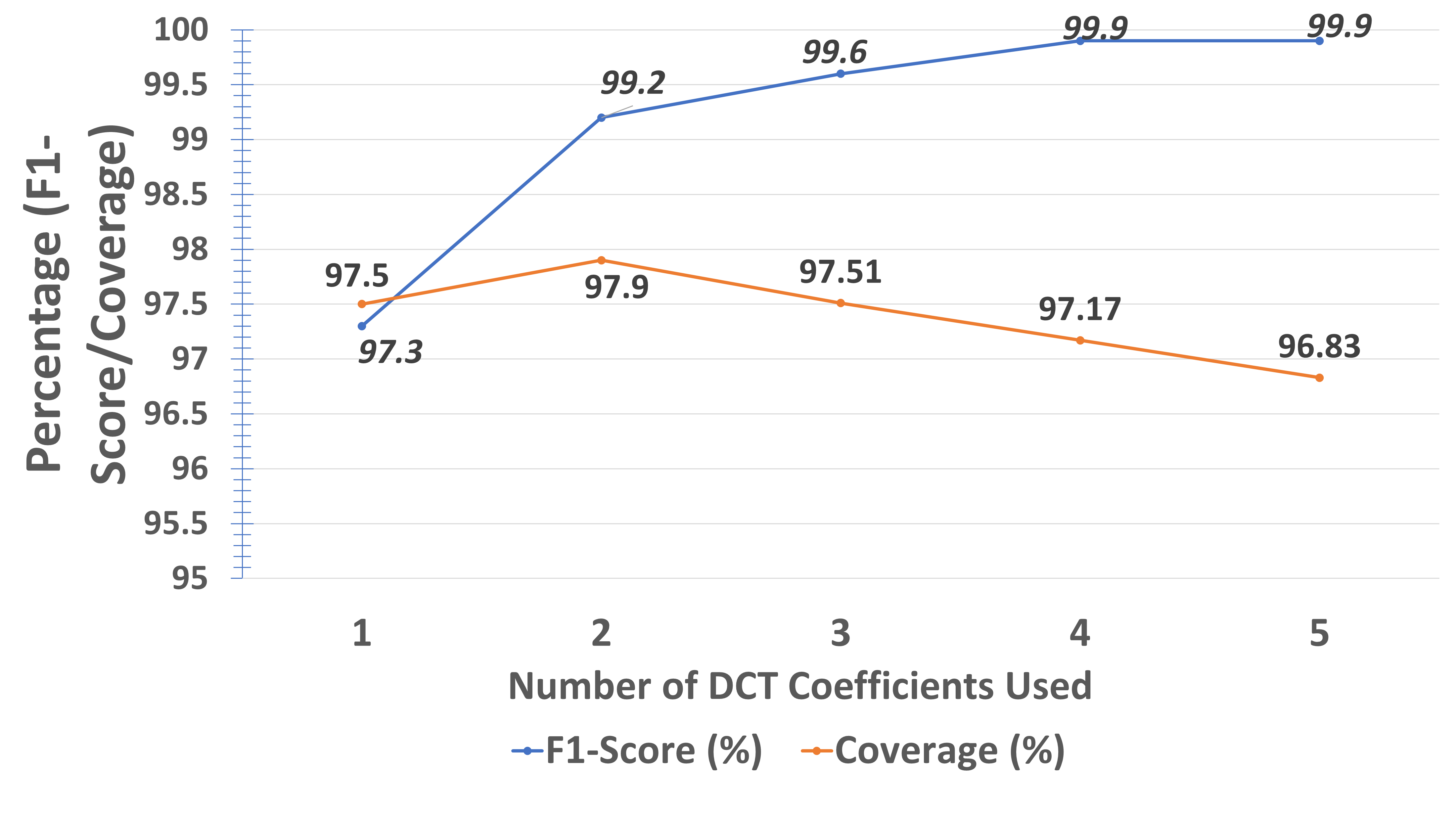
The use of multiple DCT coefficients for detection was examined for PreAct ResNet-18 on GTSRB for the input-aware backdoor attack. The detector was connected across the four residual blocks of the DNN and the final layer concurrently and the first DCT coefficients were taken for detection, . The dimensionality reduction and feature extraction via PCA were done in parallel on each row of the DCT matrix of each layer as discussed in Section 4. Outlier detection was done in parallel with an attack declared if any of the s from the DCT coefficients was an outlier with respect to its distribution using its own outlier detector. The results are shown in Figure 15. The use of more DCT coefficients marginally raises detection coverage and lowers false positive rate at the cost of overhead increases from additional computation.