Intersection formulas for parities on virtual knots
Abstract
We prove that parities on virtual knots come from invariant 1-cycles on the arcs of knot diagrams. In turn, the invariant cycles are determined by quasi-indices on the crossings of the diagrams. The found connection between the parities and the (quasi)-indices allows to define a new series of parities on virtual knots.
Introduction
V.O. Manturov [32] defined a parity as a rule to assign labels and to the crossings of knot diagrams in a way compatible with Reidemeister moves. Capability to discriminate between odd and even crossings allows to treat the crossings differently when transforming knot diagrams or calculating their invariants. The notion of parity allows to strengthen knot invariants, to prove minimality theorem and to construct (counter)examples [16, 18, 30, 31, 32, 33, 34, 35, 36].
In [17] parities with coefficients in an arbitrary abelian group were defined, and in [38] oriented parity was introduced.
A well known parity-like invariant is the index polynomial. Starting Turaev’s polynomial [43], the index polynomial has appeared numerously in papers of A. Henrich [15], Y.H. Im, K. Lee, S.Y. Lee [19], Z. Cheng [4], H. Dye [9], L.H. Kauffman [24], L.C. Folwaczny [11], J. Kim [27], M.J. Jeong [21], H. Gao, M. Xu [12], N. Petit [42], K. Kaur, M. Prabhakar, A. Vesnin [26] and others. The first axiomatization of index properties is due to Z. Cheng [5]. M. Xu [44] found the general conditions for an index to define an invariant polynomial and defined weak chord index. See also [5, 8] for other index axiomatics and examples of chord indices.
The present paper establishes a new relation between the (oriented) parity and the (weak chord) index.
The content of the paper can be described by the following diagram.
Using the technics of [40], in Section 2 we define the parity cycle of an oriented parity. In fact, the parity cycle is some labeling of arcs of knot diagrams compatible with Reidemeister moves. The intersection formula (2) establishes a bijection between parities and invariant cycles. In Section 2.3 we show how parity cycles can be constructed from a biquandle 1-cocycle (up to some issue with colouring monodromy). In Section 3 we return the labeling from arcs to crossings and prove that the parity cycle is determined by some quasi-index on the crossings of knot diagrams. Quasi-index generalizes the notion of index on crossings, and its nature is not clear yet. Section 4 is devoted to various formulas which restore a parity for a given (weak chord) index. Sections 5,6 and 7 describe how the intersection formula can be adapted to long virtual knots, parity functors and virtual links. In the last section 9 we loop the intersection formula by considering parities as (signed) indices, and define derived parities.
1 Definitions
1.1 Virtual knots
We start with the definitions of virtual knots.
A -graph is any union of four-valent graphs and trivial components, i.e. circles considered as graphs without vertices and with one (closed) edge. A virtual diagram is an embedding of a -graph into plane so that each vertex of the graph is marked as either classical of virtual vertex. At a classical vertex one a pair of opposite edges (called overcrossing) is chosen. The other pair of opposite edges at the vertex is called undercrossing.
Virtual crossings of a virtual diagram are usually drawn circled. The undercrossing of a classical vertex is drawn with a broken line whereas the overcrossing is drawn with a solid line (see Fig. 1).

Moves of virtual diagrams include classical Reidemeister moves (, , ) and detour moves () that replace any diagram arc, which has only virtual crossings, with a new arc, which has the same ends and contains only virtual crossings (see Fig. 2). An equivalence class of virtual diagram modulo moves is called a virtual link [23].


A unicursal component is a minimal set of diagram edges which is closed under passing from an edge to its opposite (at some end of the edge) edge. A virtual knot is an equivalence class of diagrams with one unicursal component.
On the other hand, virtual knots can be defined by means Gauss diagrams [13]. The Gauss diagram of a virtual knot diagram is a chord diagram whose chords correspond to the classical crossings of , see Fig. 3. The chords carry an orientation (from over-crossing to under-crossing) and the sign of the crossings, see Fig. 4.


Classical Reidemeister moves induce transformations of Gauss diagrams (see Fig. 5). Virtual knots are exactly the equivalence classes of Gauss diagrams modulo the induced Reidemeister moves.

Recall that an abstract knot diagram [22] can be constructed for a virtual knot diagram as follows. Consider a two-dimensional surface with boundary immersed in the neighbourhood of the diagram as shown in Fig. 6. Then glue discs to the boundary of this surface. Denote the obtained closed surface by .

The virtual knot diagram lifts naturally to as its -skeleton . The graph can be considered as a knot diagram on the surface in with classical crossings. The pair is the abstract knot diagram of the virtual knot diagram . We will call the graph the covering graph of the diagram .
The Gauss diagram and the covering graph of a virtual knot diagram are connected by continuous maps (Fig. 7). The projection contracts the chords of to points, and the projection is an immersion of a neighbourhood of in the surface to the plane . The double points of the projection corresponds to the virtual crossing of the diagram .

Since the surface is oriented, for any two cycles , in the graph their intersection number is defined. Any two cycles in the diagram can be uniquely lifted to cycles in the covering graph , so one can consider the intersection number . The intersection number can be calculated in the diagram as the sum of signs of the intersection points of the cycles (Fig. 8).

1.2 Parity on virtual knots
Let be an oriented virtual knot. Consider the set of the diagrams of the knot . The set can be considered as the objects of a diagram category whose morphisms are compositions of isotopies and Reidemeister moves.
For any diagrams and a morphism between them, there is a correspondence between the crossings of the diagrams. The map is a partial bijection between the crossing set because some crossing can disappear within the transformation and other crossing can appear by a first or second Reidemeister move.
Definition 1.
An oriented parity is a family of maps defined for each diagram of the knot , that possesses the following properties:
- (P0)
for any morphism and any crossing for which there exists the corresponding crossing , one has ;
- (P1)
if is a decreasing first Reidemeister move and is the disappearing crossing then ;
- (P2)
for any crossings to which a decreasing second Reidemeister move can be applied;
- (P3+)
if is a third Reidemeister move then
where are the crossings involved in the move and is the incidence index of the crossing to the disappearing triangle , see Fig. 9.

Figure 9: Incidence indices
Remark 1.
1. The properties (P1),(P2) and (P3+) can be unified in the following property: if is a decreasing first or second Reidemeister move or a third Reidemeister move, are the crossings which take part in the move and is the incidence index of the crossing to the disappearing region .
2. Oriented parities include parities with coefficients defined in [17] because those parities posses the property for any crossing so the incidence indices do not matter.
Among examples of parities are the Gaussian parity, the link parity (with coefficients in ) of virtual knots, the index parity with coefficients in and the homological parity of knots in a given surface (with coefficients in the first homology group of the surface) [18, 39].
Example 1 (Gaussian parity).
Let be a diagram of a knot and be a crossing of . The crossing splits into two oriented halves (see Fig. 10). The Gaussian parity of is the parity of the number of crossing points on any half.

For example, a diagram of a virtual eight-knot in Fig. 11 has two odd and one even crossings.

Example 2 (Link parity).
Let be a diagram of some link with two components. The crossings of the diagram can be divided into self-crossings of a component of and mixed crossings where two different components intersect. One assigns the parity to the self-crossings and the parity to the mixed crossings.
Example 3 (Index parity).
Let be a diagram of an oriented virtual knot and be a crossing of . Let us calculate the crossing points on the left half of the diagram at the crossing with the signs as in Fig. 12. The sum is the index parity of the crossing . Note that coincides with the intersection index of [15] and differs by the sign of the crossing from the index from [24]: (see also [4]).

The Gaussian parity is the reduction of the index parity.
Since the index parity does not use under-overcrossing structure, this parity is defined for flat knots.
Example 4 (Homological parity).
Let be a knot in a fixed oriented surface and be its diagram. Any crossing splits the diagram into left and right halves. This halves are cycles in the surface. The homological parity of the crossing is the element where is the homology class of the knot .
Let us remind basic properties of oriented parity [39].
Proposition 1.
Let be an oriented parity on diagrams of a knot and be a diagram of .
1. Assume that crossings form a bigon (Fig. 13 left). Then ;
2. Assume that crossings form a triangle (Fig. 13 right). Then .


Proof.
1. We need only to prove the statement for alternating bigons. Apply a first Reidemeister move as shown in Fig. 14. By the properties (P1) and (P3+) we have
and . Hence, . Since , we have and .

2. Let be the crossings of a triangle in the diagram . If a third Reidemeister move can be applied to the triangle, the equality follows from the property (P3+).

If form an alternating triangle, apply a second Reidemeister move as shown in Fig. 15. Then . By the property (P2) and the previous statement, , hence . By the property (P3+) the equality, we have
Thus, and
∎
2 Potentials and parity cycle
Let be a parity with coefficients in an abelian group on diagrams of an oriented virtual knot . Let be the category of diagrams of the knot .
Let be a virtual diagram of . An arc of the diagram is a part of which starts end ends at a classical crossing and contains no classical crossings inside. Denote the set of arcs of the diagram by . The set can be identified with the set of edges of -skeleton on the abstract knot diagram which corresponds to , or with the set of edges of the core circle of the Gauss diagram .
An isotopy or a detour move induces a bijection . A Reidemeister move induces a correspondence between the arcs: an arc corresponds to an arc if and have a common point outside the area where the move occurs. For example, for an increasing first Reidemeister move, some arc corresponds to two arcs adjacent to the loop (Fig. 16). An increasing second Reidemeister move splits some two arcs and into arcs and correspondent to and arcs and correspondent to . The small arcs participating in Reidemeister moves have no correspondent arcs.

2.1 Potentials
Definition 2.
Let be two arcs of the diagram . The potential between the arcs and is defined as the parity of the crossing produced by the second Reidemeister move applied to and (Fig. 17). By Proposition 1, the value does not depend on which arcs goes over in the Reidemeister move. Analogously, we define the potentials (Fig. 17).

For any arc we denote (Fig. 18).

Proposition 2.
- 1.
For any arcs we have
- 2.
For any arcs we have
Proof.
1. The first statement follows from the definition of potentials and property (P2).
2. Let us prove the identity . Apply second Reidemeister moves to the arcs as shown in Fig. 19. Denote the obtained diagram by . Then . By property (P3+) we have . Since , we get the required equality.

The other equalities can be proved analogously. ∎
Corollary 1.
For any arcs we have , , .
Proposition 3.
Let be the arcs incident to a crossing of the diagram as shown in Fig. 20. Then .

Proof.
Apply a second Reidemeister move as shown in Fig. 21. Let be the obtained diagram. By property (P2) , and by definition . Then . The other equalities are proved analogously.

∎
Corollary 2.
Let be the arcs incident to a crossing of the diagram as shown in Fig. 20. Then .
2.2 Parity cycle
Consider the cell complex of the covering graph of the diagram . The 0-chain space can be identified with the group which consists of linear combinations of crossings of the diagram with coefficients in the group . The group of 1-chains is identified with the group of linear combinations of arcs of with coefficients in . Having in mind these identifications, we shall write below instead of , .
Note that is the set of 1-cycles in the diagram with values in the group .
Definition 3.
Let , , be a family of 1-chains assigned to all diagrams of the virtual knot . The family of chains is invariant if for any morphism (an isotopy or a Reidemeister move) and any correspondent arcs and their coefficients coincide: .
A cycle is normalized if the intersection number .
The next theorem shows that any parity determines an invariant normalized cycle.
Definition 4.
Let be a diagram of the oriented virtual knot , and be the covering graph of the diagram . For an oriented parity with coefficients in an abelian group we define a 1-chain as follows
| (1) |
The 1-chain is called the parity cycle of the oriented parity in the diagram .
Theorem 1.
Let be an oriented parity with coefficients in an abelian group on the diagrams of an oriented virtual knot , be a diagram of , and be the parity cycle. Then
- 1.
is a genuine 1-cycle in the cell complex , i.e. ;
- 2.
is an invariant cycle;
- 3.
is normalized;
- 4.
(the intersection formula) for any crossing we have
(2)
Proof.
1) The first statement of the theorem is a reformulation of Corollary 2.
2) The invariance of is a consequence of the property (P0) of the parity . Indeed, let be a morphism of diagrams and and be correspondent arcs . Apply second Reidemeister moves as shown in Fig. 18 to the common part of the arcs. Then we get a new diagram from and a diagram from , and crossings and such that and . The morphism induces a diagram morphism which identifies the crossings and . Hence, by the property (P0) we have and .
3) Let us prove first the intersection formula. Let be a point of the diagram which is not a crossing, and , be the corresponding arc of the diagram. For any arc denote . By Proposition 2, for any the equalities hold
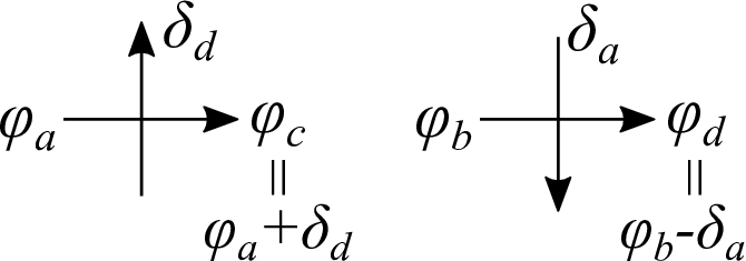
Thus, the potential changes by when passing a crossing (Fig. 22).
Now, fix a crossing (Fig. 20). The parity is equal to by Proposition 3. The arcs and are the end and the start of the left half . Hence, the difference between the potentials and is the sum
of the increments of the potential at the crossing in the left half of the diagram.
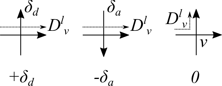
On the other hand, the intersection number is the sum of signs of the intersection points of the cycles multiplied by the values of the cycles. Shift the half to the left of . Then the intersection points correspond to the crossings in the half (Fig. 23) and the contribution of the point corresponding to a crossing is equal to . Thus,
4) Consider as a route along the diagram which starts and ends at the point . The reasonings above show that . ∎
Let us prove the inverse statement.
Theorem 2.
Let , , be an invariant normalized cycle with values in an abelian group on the diagrams of a virtual knot . Then the intersection formula
defines an oriented parity on diagrams of the knot .
Proof.
Let us check the properties of oriented parity.
(P0) Let be a Reidemeister move, and and be correspondent crossings. The coverings graph and can be considered as embedded graphs in the surface (or when is an increasing second Reidemeister move). The cycles and define elements and in and . The intersection values are the results of the intersection map
Consider the continuous map which contacts the region where the Reidemeister move occurs to a point (Fig. 24). Then . Since is homotopic to the identity map, then , and and . On the other hand, because the chain is invariant. Thus,

(P1) Let be a crossing participating in a first Reidemeister move. Then the diagram half at the crossing is either homotopic to or contractible in (Fig. 25). In both cases, because is normalized.

(P2) Let be crossings participating in a second Reidemeister move. Then the diagram is homologous to the sum of the halves and in (Fig. 26).


Then .
(P3) Let be crossings participating in a third Reidemeister move. If the incidence indices of the crossings coincide then the sum is equal either to or to in (see Fig. 27 top). If and then is equal either to or (see Fig. 27 bottom).


In all cases
.
∎
Thus, an oriented parity defines an invariant normalized cycle, and an invariant normalized cycle generates a parity. In fact, these correspondences are inverse to each other.
Proposition 4.
1. For any oriented parity the parity coincides with .
2. For any invariant normalized 1-cycle the parity cycle coincides with .
Proof.
The first statement follows from the intersection formula (2) and the definition of the parity .

∎
Remark 2.
We can reformulate Proposition 4 as follows. Given a virtual knot and an abelian group , let be the set of oriented parities with coefficients in on the diagrams of and be the set of normalized invariant cycles with coefficients in on the diagrams of . The sets and have natural structure of abelian groups. Then the intersection formula defines an isomorphism
Example 5 (constant parity cycle).
Let be an arbitrary element. Define a constant 1-chain : for all arcs . Then is an invariant cycle. The cycle is normalized because . The parity determined by the cycle is proportional to the index parity:
We have the minus in the formula because the signs in the definition of are opposite to the signs of intersection points (cf. Fig. 8 and 12).
Definition 5.
Let , , be an invariant cycle with values in the group . The signature of the cycle is defined by the formula
| (3) |
Proposition 5.
The signature of an invariant cycle is a knot invariant.
Proof.
Let be a Reidemeister move. By reasonings of Theorem 2, and in (or in if is an increasing second Reidemeister move). Hence,
and the signature is invariant under Reidemeister moves. ∎
Corollary 3.
Let be an invariant cycle. If for some diagram of the knot then for any other diagram , i.e. the cycle is normalized.
The following statement shows that any invariant cycle defines a normalized invariant cycle.
Corollary 4.
Let be an invariant cycle with coefficients in an abelian group . Denote be the factor-group by the cyclic subgroup generated by the signature, and be the canonical projection. Then is an invariant normalized cycle with coefficients in .
2.3 Parity cycle induced by a biquandle 1-cocycle
Recall that a biquandle [10] is a set with two operations which satisfy the following conditions:
- 1.
for all ;
- 2.
the maps , and are bijections of
- 3.
for any ;
For a diagram of a virtual knot , a colouring of with a biquandle is a map which obeys the colouring rule in Fig. 29 for any crossing of .

Let denote the set of colourings of the diagram . For any diagram of the same knot , there is a bijection between the colouring sets and .
Given an abelian group , one can associate cohomology groups to a biquandle [2]. Here we need only the group .
A map as called a biquandle 1-cocycle with coefficients in the group if for any the following equality holds
| (4) |
Fix a biquandle 1-cocycle with coefficients in the group . For a colouring of the diagram define a 1-chain by the formula
| (5) |
By equality (4) and the colouring rule, the chain is a 1-cycle. It is also locally invariant in the following sense.
Proposition 6.
Let is an isotopy or a Reidemeister move. Let be the colouring that corresponds to . Then for any correspondent arcs and we have .
Proof.
By definition of the bijection , we have . Then
∎
Remark 3.
The difference between invariance and local invariance of a 1-cycle comes from colour monodromy. We define the colour monodromy group of the diagram as the subgroup in the permutation group of the colouring set , formed by permutations where is an arbitrary morphism (a composition of isotopies and Reidemeister moves).
If the 1-cocycle is invariant under the action of the colour monodromy group on a given colouring :
then the 1-cycle is an invariant cycle.
In general case, one can modify the formula (5) to get an invariant 1-cycle by taking the sum over colours which belong to one orbit of the monodromy group:
or by taking the sum over all the colourings:
If the cycle (or ) is not normalized, we can reduce it to a normalized one using Corollary 4.
On the other hand, one can consider the direct sum
which is invariant under the monodromy up to permutation of the components and define an oriented parity functor with coefficients in (see Section 6).
Remark 4.
Given a biquandle 1-cocycle and a colouring , we can consider the 1-cycle and its signature . The element is invariant under Reidemeister moves, hence, the set is an invariant of virtual knots.
In fact, the invariant is closely related to biquandle cocycle invariants [2]. Recall that a biquandle 2-cocycle with coefficients in an abelian group is a map which obeys the following conditions:
- 1.
for all ;
- 2.
for all .
Given a biquandle 2-cocycle and a colouring one assigns to each positive crossing of the diagram (Fig. 29 left) the Boltzman weight , and to each negative crossing (Fig. 29 right) the weight . Then the sum
is an virtual knot invariant called the biquandle cycle invariant [2].
Note that the term is invariant under Reidemeister moves (up to identification of the colouring).
Let be the linear biquandle with operations . The following proposition can be checked by direct computations.
Proposition 7.
- 1.
Any 1-cocycle defines a biquandle 2-cocycle of the product biquandle by the formula
(6) - 2.
for any .
3 Quasi-index
Let be a virtual knot and be its diagram category. Let be an abelian group. Let be an oriented parity with coefficients in on the diagrams of the knot and , be its parity cycle.
Let be a diagram of the knot . For any crossing of the diagram (see Fig. 20) consider the element (Fig. 30)
| (7) |
Thus, we have a map .

Definition 6.
Let be a virtual knot and be its diagram category. A family of maps , is called a quasi-index on the diagrams of the knot if the following conditions hold
- (Q0)
for any Reidemeister move and any crossing which does not take part in the move, one has ;
- (Q2)
for any crossings to which a decreasing second Reidemeister move can be applied;
- (Q3)
if are the crossings which take part in a third Reidemeister move then there exists an element such that
where is the incidence index of the crossing to the disappearing triangle .
A quasi-index is called an index on the diagrams of the knot if the terms in condition (Q3) are equal to for all third Reidemeister moves on the diagrams of . In other words, third Reidemeister moves do not change the indices of the correspondent crossings.
Remark 5.
Theorem 3.
Let be a virtual knot and be an oriented parity with coefficients in a group on the diagrams of the knot . Let be the parity cycle of and , , be the map defined above. Then
- 1.
the family of maps is a quasi-index on diagrams of the knot ;
- 2.
for any diagram there is a unique element such that
(8)
Proof.
1. Let us check the quasi-index properties.
The property (Q0) follows from the invariance of the parity cycle .
Let and be two crossings participating in a second Reidemeister move (Fig. 31). Let be the values of the parity cycle on the arc incident to . By definition, and . Thus, . The other type of second Reidemeister move can be checked analogously.

Let be the crossings participating in a third Reidemeister move and be the corresponding crossings in the diagram . Then and . By definition,
Hence,
Let . Then . Thus, the condition (Q3) is fulfilled.
Other cases of third Reidemeister move can be checked analogously.

2. Let be a diagram of the knot , be its covering graph, and be its Gauss diagram. We use a non standard orientation of the chords of : from the undercrossing to the overcrossing for the chords corresponding to positive crossings of , and from the overcrossing to the undercrossing for the negative chords.
The parity cycle can be considered as a 1-cycle on the Gauss diagram . The labels of on the core circle of come from the labels on the edges of , i.e. on the long arcs of the diagram . Then the labels of on the chords of coincide with quasi-indices of the correspondent crossings (see Fig. 33).

Each (oriented) chord of defines a 1-cycle which corresponds to the right half of the diagram at the crossing (Fig. 34).

Now, let us consider the cycle . The values of on the chords are zero, then is a cycle on the core circle of the Gauss diagram. Hence, the values of on the arcs of the core circle are all equal to some element . Then and
∎
Definition 7.
The quasi-index defined by the formula (7) is called the parity quasi-index of the parity . The element is called the reminder of the parity .
Remark 6.
We can give a topological interpretation of the equality (8). Let be the cell complex obtained from by gluing a 2-cell to the core circle. Then is homotopically equivalent to the bouquet of circles . The inclusion map induces an exact sequence in homology
But is isomorphic to , and is equal to . Thus, we have the exact sequence
| (9) |
The correspondence , , defines a splitting of this exact sequence. Thus, .
Corollary 5.
Let be an oriented parity with coefficients in on diagrams of the knot , and be the parity quasi-index of . Then for any diagram and any crossing
| (10) |
Thus, the parity of a crossing is defined by the parity quasi-index and the reminder term . Let us look how the reminder changes under Reidemeister moves.
Proposition 8.
Let be an oriented parity with coefficients in on diagrams of the knot , and be the reminder of .
- 1.
Let be an increasing first Reidemeister move, and be the new crossing. Then
where the coefficient depends on the type of the appeared loop (Fig. 35):
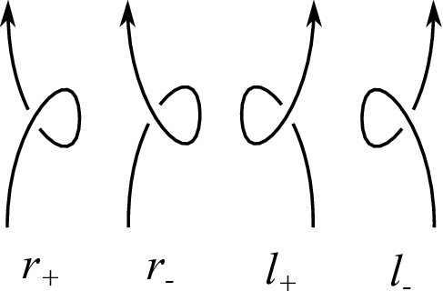
Figure 35: Types of loops - 2.
Let be an increasing second Reidemeister move, and be the new crossings. Then
- 3.
Let be a third Reidemeister move applied to crossings , and be the corresponding crossings in . Then
where is the term in property (Q3) and the coefficient is determined by the type of the third Reidemeister move (Fig. 36).


Figure 36: Types of third Reidemeister moves
Proof.
The change of the reminder under a Reidemeister move is determined by the invariance condition of the parity cycle .
The diagrams and can be lifted to the abstract knot diagram , and their lifts differ only in the region where the Reidemeister move occurs. Just like in Theorem 2, consider a map which contracts this region to a point, and let . The map induces maps of 1-chains from and to which we denote by . Then , for all crossings , and by the invariance of .
1. Let be an increasing first Reidemeister move with the new crossing . Then
But for loops of type and for loops of type . Then . Hence, .
2. Let be an increasing second Reidemeister move, and be the new crossings. Then by properties (Q0) and (Q2) we have
But , hence, .
3. Let be a third Reidemeister move applied to crossings , and be the corresponding crossings in . Since and , we have
The sum is equal to (see Fig. 36). Hence, . ∎
Remark 7.
Proposition 8 means that the reminder and hence the parity cycle are determined by the quasi-index up to constant summand . We can eliminate the ambiguity if we set the value for an arbitrary diagram .
Let us give an example of a quasi-index which is not an index.
Example 6.
Consider the biquandle with the operations given by the matrices
and the 1-cocycle such that , and . The biquandle is isomorphic to the biquandle with , and for .
Consider the coloring of the unknot diagram with given in Fig. 37 left. Let be the corresponding locally invariant cycle. Since is an unknot diagram, the cycle is normalized. Let be the quasi-index of the cycle . Then the quasi-indices of the crossings participating in the third Reidemeister move in Fig. 37 change from , , to , , . Then . Thus, is not an index.

Note that this example is not quite correct because is not invariant due to the colouring monodromy and does not define a parity. Figure 38 implies that one can interchange the colours and in any diagram of the unknot but the cocycle is not invariant under this permutation.

The biquandle with the cocycle can define a parity with an invariant cycle whose quasi-index is not an index, for a knot which has a colouring with such that it has an edge coloured with (or ) and its orbit under the colouring monodromy group is trivial: for such a knot we take its connected sum with the unknot diagram in Fig. 37. Such a knot could be found among irreducible odd knots in the sense of [31] but the author do not know an explicit example.
Remark 8.
Let be a virtual knot, be a biquandle and be a cocycle which defines an oriented parity with coefficients in on the diagrams of the knot . Then the following conditions ensure that the quasi-index of the parity is an index on the diagrams of : for all
| (11) | |||
The conditions above come from the equations for the crossings participating in third Reidemeister moves.
Now, let be an arbitrary quasi-index on the diagrams of a virtual knot with coefficients in an abelian group . Fix a diagram of the knot and an element . Using the formulas of Proposition 8, we can extend the reminder to other diagrams of , and define the cycle by the formula (8). There are two obstacles for to be a normalized invariant cycle and define a parity. The first one is the monodromy.
Let be a diagram morphism, i.e. a sequence
of Reidemeister moves . Define the monodromy of the morphism as the sum
where is determined by Proposition 8. The set
is called the monodromy group of the quasi-index . Note that is a subgroup in and it does not depend on the choice of the diagram of the knot .
If the monodromy group is not zero then the cycle is ambiguous because Reidemeister moves can shift the reminder by any element of .
Example 7.
Consider the constant quasi-index with coefficients in on the unknot diagrams. Take the diagram in Fig. 39 and set . Consider the morphism which consists of two first, one second Reidemeister move and detour moves (Fig. 39). Then . Hence, the monodromy group coincides with the coefficient group .

The other obstacle for is the signature of the quasi-index.
Definition 8.
Let be an quasi-index on the diagrams of a virtual knot with coefficients in an abelian group . Let be a diagram of . Then the signature of the quasi-index is defined by the formula
| (12) |
Note that where is defined by formula (8) with any choice of .
Proposition 9.
Let be an quasi-index on the diagrams of a virtual knot with coefficients in an abelian group . Then the signature is invariant under Reidemeister moves.
Proof.
Thus, if the signature of the quasi-index is not zero then the cycle is not normalized. But we make it normalized like in Corollary 4. Thus, we have
Theorem 4.
Let be an quasi-index on the diagrams of a virtual knot with coefficients in an abelian group . Let and be the signature and the monodromy group of . Consider the factor-group
Then the formula
| (13) |
defines an oriented parity with coefficients in on the diagrams of the knot .
On the other hand, any quasi-index defines an oriented parity functor with coefficients in (see Theorem 11).
We postpone the study of quasi-indices to further papers and concentrate below only on indices.
4 From index to parity cycle
By Definition 6, we can define an index on the diagrams of of a virtual knot with coefficients in an abelian group as a family of maps , , such that
- (I0)
for any Reidemeister move and any crossings and such that , one has ;
- (I2)
for any crossings to which a decreasing second Reidemeister move can be applied.
As in the previous section, our goal is to construct an invariant 1-cycle and a parity for a given index .
Let be an index on the diagrams of of a virtual knot with coefficients in an abelian group . Let be a diagram of the knot . Define a -cycle by the formula
| (14) |
By property (I0), the 1-cycle is invariant under third Reidemeister moves.
Let be an increasing second Reidemeister move and , , be the new crossings. By property (I2), , and Proposition 8 implies that
in . In order to compensate the increment of the cycle , we modify the formula (14).
Let and be the sets of negative and positive crossing in . For any crossing define its signed halves by the formulas , .
Consider the 1-cycle
Thus,
| (15) |
By definition of , the following proposition holds.
Proposition 10.
The cycle is invariant under second and third Reidemeister moves.
Remark 9.
We can consider the cycle which is also invariant under second and third Reidemeister moves. The difference between and
is expressed using the linking invariant of the index (see Section 9).
Let us consider an increasing first Reidemeister move and let be the new crossing. There can be four types of the crossing , see Fig. 35. By property (I0), there are elements which are the index values of the corresponding types of loop crossings. Due to Whitney’s trick and property (I2), and . Thus, the index coincides with one of two values or .
The increment of the 1-cycle for the move is equal to
where if is of type , for and , and for the type . Hence,
| (16) |
We can consider several strategies to deal with first Reidemeister moves (some of them fit to quasi-index case):
4.1 Reduced index
By equation (16) the invariance under first Reidemeister move takes place automatically if we are lucky enough to have .
Definition 9.
An index on diagrams of a virtual knot with coefficients in an abelian group is -reduced if the index value of the crossings of types and (Fig. 35) is zero: .
Analogously, the index is -reduced if the index values of - and -crossings is zero: . And is R1-reduced if .
Theorem 5.
Let be an -reduced index on diagrams of a virtual knot with coefficients in an abelian group . Then the formula (15) defines an invariant 1-cycle and the formula
| (17) |
defines an oriented parity on diagrams of the knot with coefficients in the group , where is the signature of the index .
For a general index , we can either suppress or evade the index value . The following statement (cf. Theorem 4) represents the first option.
Corollary 6.
Let be an index on diagrams of a virtual knot with coefficients in an abelian group and let be the index value of the crossings of types and . Then the formula (15) defines an invariant 1-cycle and the formula (17) defines an oriented parity on diagrams of the knot with coefficients in the group , where is the signature of the index .
Definition 10.
Given an index on diagrams of a virtual knot with coefficients in an abelian group , define its -reduction as the a family of maps ,, set by the formula
Here is the index value of the crossings of types and .
The following statement is evident.
Proposition 11.
The -reduction is an -reduced index on diagrams of with coefficients in .
Hence, Theorem 5 holds for . We can reformulate it as follows.
Corollary 7.
Let be an index on diagrams of a virtual knot with coefficients in an abelian group and let be the index value of the crossings of types and . Then the formula
| (18) |
defines an invariant 1-cycle and the formula
| (19) |
defines an oriented parity on diagrams of the knot with coefficients in the group , where is the signature of the -reduction .
One can consider the reduced 1-cycle is a distant analogue of odd writhe polynomial [4].
Remark 10.
Analogous results take place when the index is -reduced, i.e. .
We will return to the case of reduced indices in Section 9.
4.2 Almost classical knots
Let us recall the definition of almost classical knot [1].
Definition 11.
A virtual knot diagram is called almost classical if for any crossing its index parity is zero: . Equivalently, a diagram is almost classical iff .
A virtual knot is almost classical if it has an almost classical diagram.
The category of almost classical diagrams embeds in the category of virtual knot diagrams and Reidemeister moves between them in the following sense: if and are almost classical diagrams of one knot then there exist a sequence of Reidemeister moves such that all the intermediate diagrams are almost classical. This fact can be proved by using parity projection [18]. Denote the set of almost classical diagrams of by .
The condition in the definition of almost classical knots means we need not to worry about the invariance of the cycle . Theorem 4 and definition of almost classical diagrams imply the following result.
Theorem 6.
Example 8.
Let be the virtual knot 5.2012 (Fig. 40). It is almost classical [1]. Consider the reduced stable parity on the knot [41]. The based matrix of the diagram in Fig. 40 is primitive. Each crossing of defines a nonzero primitive tribe. Taking into account the signs of crossings, there are no nontrivial symmetries of the diagram and the based matrix . Then we can define an index with coefficients in such that the crossings of correspond to the basis of . Then the parities , , correspond to the rows of the based matrix (without the first row and the first column).

4.3 Regular virtual knots
Let us consider virtual knot diagrams up to regular isotopy of classical crossings, i.e. up to all moves except R1.
Definition 12.
A regular virtual knot is an equivalence class of virtual knot diagrams modulo isotopies, second and third Reidemeister moves and detour moves.
Thus, we do not have first Reidemeister moves and do not need to check invariance under them. Note also, that the statements of Sections 2 and 3 can be proved without first Reidemeister move. Then we can formulate the theorem.
Theorem 7.
4.4 Rotational virtual knots
An analogous result can be obtained if one forbids first virtual Reidemeister moves (instead of first classical Reidemeister moves).
Definition 13.
A rotational virtual knot [25] is an equivalence class of virtual knot diagrams modulo isotopies, classical Reidemeister moves and regular detour moves (i.e. moves which includes virtual analogues of second and third Reidemeister move but not first Reidemeister move).
Let be a diagram of a rotational virtual knot . Then can be considered as plane diagram. In rotational knot theory, the writhe and the rotation number of the diagram can be changed only by a first classical Reidemeister move.
Let be an increasing first Reidemeister move and be the new crossing. Then we have the following table.
| Type | ||||
|---|---|---|---|---|
The table shows that the writhe and the rotation number can be used for correction of the 1-cycle .
Theorem 8.
Let be a rotational virtual knot and be an index on diagrams of with coefficients in an abelian group . Then the formula
| (20) |
defines an invariant 1-cycle and the formula
| (21) |
defines an oriented parity , , on the rotational knot with coefficients in the group , where is the signature of the index .
5 Intersection formula for long knots
Let us recall the definition of long virtual knots [37].
Definition 14.
A long virtual knot diagram is an immersion in general position of the oriented line into the plane which coincides with the axis outside some sufficiently large disc; and each crossing is marked as either classical or virtual crossing, see Fig. 41.
A long virtual knot is an equivalence class of long virtual knot diagrams modulo isotopies, Reidemester moves and detour moves.

Definition 15.
Given a crossing of a long knot diagram , the oriented smoothing at splits the diagram into the open half of at the crossing and the closed half of at , see Fig. 42.

For a crossing of the diagram define its order as follows [6]: if , and if .
For example, the orders of the classical crossings of the diagram in Fig. 41 are (from left to right) .
Remark 11.
The results of Sections 2 and 3 holds for long knots with two main differences.
- 1.
Since a long knot is not closed, there is no normalization condition on the parity 1-cycle.
- 2.
Using closed halves, one can localize the increments which the parity quasi-index produces in formula (8) under Reidemeister moves, and resolve the problem of constructing the parity cycle from the parity quasi-index.
Theorem 9.
1. Let be an oriented parity with coefficients in an abelian group on the diagrams of a long virtual knot . Then formula (1) defines an invariant 1-cycle such that
| (22) |
2. Given an invariant 1-cycle on diagrams of a long virtual knot with coefficients in an abelian group , then the formula
defines an oriented parity on on diagrams of with coefficients in .
Theorem 10.
1. Let be an invariant 1-cycle on diagrams of a long virtual knot with coefficients in an abelian group . Then formula (7) defines a quasi-index on diagrams of with coefficients in such that
| (23) |
for some and any diagram .
2. Let be a quasi-index on diagrams of a long virtual knot with coefficients in an abelian group , and be an arbitrary element. Then formula (23) defines an invariant 1-cycle on diagram of the knot with coefficients in and the formula
| (24) |
defines an oriented parity on diagrams of with coefficients in .
Proof.
1. Let be an invariant 1-cycle on diagram of the knot with coefficients in . By Theorem 3, formula (8) and definition of closed halves, the family of maps is a quasi-index and
Let be the initial arc of the diagram . Since belongs to neither halves , , the value of the cycle on the arc is equal to . Then by invariance of , the value does not depend on the diagram . Thus, and we get the formula (23).
2. Let be a quasi-index on diagrams of with coefficients in . Define a 1-cycle by formula (23). Let us prove its invariance.
Let be a Reidemeister move. By Proposition 8 and definition of closed halves, we have
where is the intermediate graph in the surface , see the proof of Proposition 8. Let ad be the initial arcs of and . Then . Since does not belong to any closed half, for any and . Analogously, . Hence,
Thus, , and the cycle is invariant.
Example 9.
Let be the biquandle with operations , , , and be the biquandle 1-cocycle given by the formula , .
Consider the long knot diagram in Fig. 41. Choose the colouring such that where is the initial arc of (Fig. 43). Then we have a 1-cycle . The corresponding quasi-index is constant .

The cycle is induced by formula (23) with the quasi-index and . The values of the parity on the crossings are (from left to right) that coincide with the values of the index parity .
6 Intersection formula for parity functors
Let and be two abelian groups. A partial isomorphism between and is a group isomorphism where and are some subgroups.
Recall the definition of an oriented parity functor [39].
Definition 16.
An oriented parity functor on the diagrams of a virtual knot is a family of pairs , , where is an abelian group and is a map from the set of crossings of the diagram , such that for any isotopy or a Reidemeister move a partial isomorphism between and is fixed, and
- (P0)
for any corresponding crossings and we have ;
- (P1)
if is a decreasing first Reidemeister move and is the disappearing crossing;
- (P2)
if is a decreasing second Reidemeister move and are the disappearing crossings;
- (P3+)
if is a third Reidemeister move then
where are the crossings involved in the move and is the incidence index of the crossing in relation with the disappearing triangle.
Given an oriented parity functor , , denote by the subgroup generated by the elements , , in the coefficient group . The parity functor is called reduced if for all diagrams of the knot .
Remark 12.
1. Each parity with coefficients in a group is a parity functor with , and .
2. A parity functor assigns to any diagram its own coefficient group where the parity values lie, and these groups are identified by partial isomorphisms for diagrams connected by a Reidemeister move. This makes parity functors more flexible comparing to parities. For example, parity functors can assimilate monodromy of quasi-indices.
Theorem 11.
Let be a quasi-index with coefficients in an abelian group on diagrams of a virtual knot . Denote where is the signature of the quasi-index . Then the family of maps given by the formula
| (25) |
defines an oriented parity functor on diagrams of the knot with coefficients in the groups . For a Reidemeister move the isomorphism is defined by the formula
where is determined by Proposition 8.
Proof.
The properties (P1)–(P3+) hold because the right-hand side of the formula (25) is the intersection of the half with a normalized 1-cycle.
Let us check the property (P0). Let be a Reidemeister move, and be corresponding crossings. Denote . By Proposition 8 we have
Then
i.e. . ∎
Let us show how intersection formula manifests itself for parity functors.
Let be an oriented parity functor on diagrams of a virtual knot . Given a diagram of the knot , construct the extended diagram by applying second Reidemeister moves as shown in Fig. 18 on every arc of the diagram . The coefficient group is called the extended coefficient group of . Then the formula (1) defines a 1-cycle
Then the formula (8) defines a quasi-index .
Remark 13.
1. Let be a diagram of the knot . By definition, there is a sequence of increasing second Reidemeister moves . The morphism induces the monomorphism . The subgroup is generated by the elements , , which correspond to the crossings of the diagram , and the parities , , which can be identified with the values , , and correspond to the arcs of the diagram .
2. If is an increasing first or second Reidemeister move, then there is a sequence of increasing first and second Reidemeister moves , see Fig 44. Then the map induces a monomorphism .

The subgroup includes the values , , so we can use the map to formulate the invariance condition for the cycle (see Theorem 12).
3. Let be a third Reidemeister move. Then there is no a direct Reidemeister move between the diagrams and but there are intermediate diagrams and (Fig. 45) connected by a third Reidemeister move . The diagrams and are obtained from and by applying increasing second Reidemeister moves on the arcs and of the triangle of the move .

The move induces the group isomorphism
The moves allows to identify the group with the subgroup in generated by values for all arcs except the arcs . An analogous statement holds for . Thus, the map allows to identify the values , , with the values , .
Hence, induces a correspondence between the quasi-index values and for all crossings which do not take part in the move . Note that, does not belong to the subgroup in general because it is expressed using the values and . Then the value can not be compared with the value . By the same reason, one can not compare with and with .
On the other hand, , so we can compare its image under the isomorphism with the element (see Theorem 12).
This fact gives an explanation why for the maps it is natural to consider the conditions of quasi-indices but not of indices.
Theorem 12.
Let be an oriented parity functor on diagrams of a virtual knot . Then the chain defined above possesses the properties
- •
is a cycle, i.e. ;
- •
is invariant, i.e. for any Reidemeister move and any correspondent arcs and one has
- •
is normalized, i.e. .
The family of maps defined above possesses the properties
- (Q0)
for any Reidemeister move and any correspondent crossings and one has ;
- (Q2)
for any crossings to which a decreasing second Reidemeister move can be applied;
- (Q3)
if are the crossings which take part in a third Reidemeister move and are the corresponding crossings in then for any one has
where is the incidence index of the crossing to the disappearing triangle .
The quasi-index and the cycle are connected by the formula
with a unique .
Let us formulate an inverse statement.
Definition 17.
Let be a virtual knot and be the category of its diagrams. A tribal system is a family of partitions of the sets , , into subsets called tribes such that
- (T0)
Let be a Reidemeister move, and and be the correspondent crossings in . Then if and belong to one tribe in then and also belong to one tribe in ;
- (T2)
If is a decreasing second Reidemeister move and and are the disappearing crossings then and belong to one tribe in .
Remark 14.
1. Tribal system are in the same sort of relationship with indices as parity functors with parities. Given a quasi-index on diagrams of a virtual knot with coefficients in a group , consider the partitions where , , is the quasi-index map. Then is a tribal system on the diagrams of the knot .
2. Property (T0) implies that any Reidemeister move induces a partial bijection where if there exists such that .
3. Given a tribal system , the sign function splits any tribe , , into two subsets and we call phratries. By definition
The phratries and are called dual.
We can refine the properties (T0) and (T2) as follows:
- ()
for any Reidemeister move and any crossings such that the crossings and exist, if and belong to one phratry then and belong to one phratry too.
- ()
If is a decreasing second Reidemeister move and and are the disappearing crossings then and belong to dual phratries.
Let be a tribal system on the diagrams of a virtual knot . Consider the family of maps , , given by the formula if . The maps satisfy the conditions
- •
for any Reidemeister move and any correspondent crossings and we have ;
- •
If is a decreasing second Reidemeister move and and are the disappearing crossings then .
Denote the groups by . For any Reidemeister move the partial bijection induces a partial isomorphism .
Define the signature of the tribal system as the elements
| (26) |
Then for any Reidemeister move we have .
Consider the groups , .
Given a Reidemeister move , define partial isomorphisms by the formulas:
- •
if is an increasing first Reidemeister move and is the new crossing then we set
where if the loop crossing is of types or , and if is of type or ;
- •
if is a decreasing first Reidemeister move and is the disappearing crossing then we set
where if the loop crossing is of types or , and if is of type or ;
- •
if is an increasing second Reidemeister move and are the new crossings then we set
- •
if is a decreasing second Reidemeister move and are the disappearing crossings then we set
- •
if is a third Reidemeister move then we set
Note that the map is defined not for all elements .
Theorem 13.
Let be a tribal system on the diagrams of a virtual knot . Then the formula
| (27) |
defines a normalized invariant 1-cycle (in the sense of Theorem 12).
The formula
| (28) |
defines an oriented parity functor on diagrams of the knot with coefficients in the groups .
The theorem can proved with the reasoning of Theorem 11.
7 Parity cycle and parities on virtual links
Let be an oriented virtual link with components, and be the category of its diagrams. Let be an abelian group.
Let be an oriented parity on the diagrams of the link with coefficients in the group .
Given a diagram , one can define the parity cycle by the formula (1). Using the reasonings of Theorem 1, one can prove that is a normalized invariant cycle. The normalization condition for links takes the form:
for any component of the link diagram .
On the other hand, the intersection formula (2) does not work in general because there is no notion of a knot half for a mixed crossing in a link. Nevertheless, the parity cycle defines some kind of relative parity (for relative parities see [28]). More precisely, the following theorem hold.
Theorem 14.
Let be a diagram of an oriented virtual link , and be an oriented parity on the diagrams of the link with coefficients in an abelian group . Let be the parity cycle of .
- 1.
For any self crossing of a component its parity is equal
(29) where is the left half of the component at the crossing .
- 2.
For any crossings and of components and denote the path from to in (along the orientation of the component) by , and the path from to in by (Fig. 46). Let . Then
(30) 
Figure 46: Paths and where and are the incidence indices of the crossings and to the cycle (see Fig. 47).

Proof.
The proof of the first statement of the theorem repeats the proof in Theorem 1.
Like in Theorem 1, fix an arc of the diagram and define the potential function on the arcs of .
Let and of components and . Denote arcs incident to and by , , , as shown in Fig. 48. By Proposition 3 and . By the proof of Theorem 1 and . Then
because and .

The proof for other configurations is analogous. ∎
Example 10 (Link parity).
Let be an oriented virtual link with components, and be an abelian group. Choose an arbitrary -vector in . Denote also .
Let be a diagram of the link . For a crossing of components and (Fig. 49), its link parity is defined by the formula
| (31) |

Then by definition for any self-crossing if . Hence, the parity cycle of the link parity is trivial: . Thus, a parity on links can not be restored from the parity cycle in general.
We can specify relation between parities and parity cycles with the following proposition.
Proposition 12.
Let be an oriented virtual link with components, and let be an abelian group. Let be oriented parities on the diagrams of the link with coefficients in the group , and and be the parity cycles. Then if and only if for some .
Proof.
If then .
Assume then the parity has zero parity cycle. For any take a diagram of the link such that the components and intersect at a crossing . Denote . By property (P0) and Theorem 14 the value does not depend on the choice of the crossing and the diagram . Thus, the parity of any crossing depends only on the components which intersect at this crossing, and is equal to some .
Property (P3+) applied to the configuration in Fig. 50 implies that for all .

Denote , . Then and for all . Thus, with . ∎
Remark 15.
We can reformulate the proposition above as follows (cf. Remark 2). Let be the set of oriented parities with coefficients in on the diagrams of the link and be the set of normalized invariant cycles with coefficients in on the diagrams of . The formula (1) defines a homomorphism
Proposition 12 states that is the subgroup consisting of link parities. Note that .
On the other hand, the example below shows that in general the map is not an epimorphism.
Example 11.
Let be the diagram of a link with three components shown in Fig. 51 left. Consider a constant 1-cycle on with coefficients in : for any arc . Then is a normalized invariant cycle.

Assume that there is a parity with coefficients in such that . Apply a second Reidemeister move to get a diagram with a crossing (Fig. 51 middle). There are two second Reidemeister moves and from to the diagram shown in Fig. 51 right such that , . Then by property (P0) . But by the formula (30) we have . Thus, there is no parity whose parity cycle is .
Note that this contradiction can be avoided if one considers parity functors.
8 Intersection formula for flat knots
Recall that a flat link is an equivalence class of virtual diagrams modulo isotopies, Reidemeister and detour moves, and crossing switches (Fig. 52). In other words, flat links ignore the information on under- and overcrossing.

The reader may be noted that most of results of Sections 2 and 3 (including Theorems 1, 2, 3 and 4) hold for flat knots. On the other hand the formula (15) and the derived ones do not fit for flat knots because flat knots have not the sign function.
Let be a flat knot, and be an index on the diagrams of the knot with coefficients in an abelian group . Note that loop crossings (Fig. 35) in flat knot diagrams has only one index value that we denote by . Let us formulate an analogue of Corollary 7 for flat knots.
Theorem 15.
Let be an index on diagrams of a flat knot with coefficients in an abelian group and let be the index value of the loop crossings. Then the formula
| (32) |
defines an invariant 1-cycle and the formula
| (33) |
defines an oriented parity on diagrams of the flat knot with coefficients in the group , where
and if the floor function.
Proof.
Property (I0) of the index implies invariance of by isotopies and third Reidemeister moves. By definition, is invariant under first Reidemeister moves.
Let be an increasing second Reidemeister move and be the new crossings. If then the expressions for and coincide up to replacement with and with . Thus, for any correspondent arcs and .
Let . For all , , we have , and . Then the difference between and is equal to
Since the chain vanishes outside the region where the move occurs, we have for any correspondent arcs and . ∎
9 Derived parities of virtual knots
In this section we look at connection between parities and indices from another (and more direct) side. This will allow us to loop the intersection formula and define derived parities.
9.1 Signed index
Note that an (oriented) parity is not an index in general. Let us introduce an intermediate notion between parities and indices. Let be a virtual knot and be the category of its diagrams. Let be an abelian group.
Definition 18.
A signed index on the diagrams of the knot with coefficients in is a family of maps , , which obeys the properties
- (I0)
for any Reidemeister move and any crossings and such that , one has ;
- (I2+)
for any crossings to which a decreasing second Reidemeister move can be applied.
Let us list some simple properties of signed indices.
Proposition 13.
- 1.
Any oriented parity is a signed index;
- 2.
The sign function is a signed index with coefficients in ;
- 3.
If is a signed index with coefficients in a group and is a signed index with coefficients in a group then their product where
is an index with coefficients in ;
- 4.
If is a signed index with coefficients in a group and is an index with coefficients in a group then their product is a signed index with coefficients in .
Note that if is an index with coefficients in and is an index with coefficients in then is an index with coefficients in .
Definition 19.
Let and be groups. A map is called odd if for any in , and the map is called even if for any .
By definition, if is a group homomorphism then is odd.
Proposition 14.
Let be a signed index with coefficients in a group and be a map to another group . Then
- •
if is odd then is a signed index with coefficients in ;
- •
if is even then is an index with coefficients in .
If be an index with coefficients in and be an arbitrary map then is an index with coefficients in .
Example 12.
Let be an oriented parity with coefficients in an abelian group . Then its product with the sign function is an index. If is an index with coefficients in then is a signed index. For a signed index , the product is an index.
If (for example, is the index parity) then the modulus (, ) of the parity is an index. The sign of the parity where , is a signed index with values . The signed index can be used as a substitution for the crossing sign in the case of flat knots.
9.2 Linking invariant
Let be a signed index on diagrams of a virtual knot with coefficients in an abelian group . Denote the value of on the loop crossings of type (see Fig. 35) by , and the value of crossings of type by . Then the crossings of type have the signed index and the crossings of type have the signed index .
Definition 20.
The signed index is called R1-reduced if .
Note that any parity is R1-reduced.
Proposition 15.
Let be an R1-reduced signed index on diagrams of a virtual knot with coefficients in an abelian group . Then the value
| (36) |
is invariant under Reidemeister moves
Proof.
Let be an increasing first Reidemeister move and be the new crossing. Then
where because is R1-reduced.
Let be an increasing second Reidemeister move and be the new crossings. Then
because .
For a third Reidemeister move we have
∎
Definition 21.
For an R1-reduced signed index , the invariant is called the linking invariant of the signed index .
It is an R1-reduced index on diagrams the knot with coefficients in , we define its linking invariant as the linking invariant of its product with the sign function: . Then
| (37) |
for any diagram of the knot .
Example 13.
Let be a diagram of a two-component link . Consider the index with coefficients in given by the formula
Then is an R1-reduced index, and its linking invariant
is the linking number of the link .
Remark 17.
Let be a signed index on diagrams of with coefficients in . If is not R1-reduced define its R1-reduction by the formula
Then is an R1-reduced signed index with coefficients in . We define the reduced linking invariant by the formula
| (38) |
Another way to define a linking invariant for an unreduced signed index is to take the factor-group and consider the signed index that is the composition of with the natural homomorphism . By definition, the signed index is R1-reduce, and we can define the linking invariant .
For an index on diagrams of with coefficients in , we define the reduced linking invariants and as the invariants of the signed index .
Example 14.
Let be an index on diagrams of a virtual knot with coefficients in an abelian group . Consider the map , , . Then be an index with coefficients in . The linking invariant is called the odd index polynomial of the index . For a signed index , we define the odd index polynomial by .
9.3 Inner product of parities
The linking invariant allows to define an invariant inner product on the space of parities.
Definition 22.
Let be an oriented parity on diagrams of a virtual knot with coefficients in an abelian group , and be an oriented parity on diagrams of with coefficients in an abelian group . Define the inner product of the parities and as the linking invariant of the index :
| (39) |
Analogously, one can define the inner product of any R1-reduced (signed) index with any (signed) index.
Remark 18.
1. The formula (39) defines a bilinear map
where () is the abelian group of oriented parities on diagrams of with coefficients in ().
If is a ring (for example, ) then becomes an -module with the inner product .
2. The signature of an index with coefficients in is equal to the inner product with the index parity :
9.4 Derived parities
Definition 23.
Let be oriented parity on diagrams of a virtual knot with coefficients in an abelian group . Then is an R1-reduced index, and by Theorem 5 it defines the oriented parity with coefficients in the group . We call the parity the derived parity to the parity .
We can iterate the definition and get the series of derivations of the parity with coefficients in . Note that the coefficient groups are connected with epimorphisms .
Remark 19.
Fix a diagram of the knot . Then for the values an oriented parity on diagrams of with coefficients in is determined by the vector .
Let be the intersection matrix (with the elements in ). By formula (19) the vector of values of the derived parity is equal to
For the higher derivation we have the formula .
The coefficients of the intersection matrix can be calculated with the formulas from [43].
Example 15.
Let be a virtual knot and be the index parity on with coefficients in . Denote the derivations of the index parity by , , and let be the coefficient group of . Denote and . Note that .
Calculations of the derived parities for virtual knots with number of crossings demonstrate several patterns.
1. (degeneration) Consider the knot 3.1 (Fig. 53). The signature of derived parities are equal , and . Then for all , and the parities , , vanish. The odd index polynomials are
Another degeneration example is given by the knot 3.5. For this knot, the signatures are and for . Then for . On the other hand, , so for all . The odd index polynomials are


2. (stabilization) Consider the knot 2.1. Then and for . Then for . For the derived parities are equal to . The odd index polynomials are
3. (periodicity) Consider the knot 4.1. For this knot, and for . Then , . The sequence of derived parities has period : , , , , . (The numeration of the crossings coincides with that in the Gauss code in the Green’s table of virtual knots [14].) The odd index polynomials are
4. (growth) Consider the knot 4.75. Then for all , hence, , . The parity vector appears to be the eigenvector of the intersection matrix with the eigenvalue . Thus, . The odd index polynomials are all zero: , .
The knot 4.107 gives an example of growth with periodicity. For this knot, for all , and and , . The odd index polynomials are
Example 16.
Consider the knots 2.1 and 4.4 from the table [14]. We denote them by and . Then but and are different. Thus, the derived index polynomials can be more sensitive than the conventional one.
On the other hand, if index parity is trivial () then the derived parities are also trivial. This situation occurs for almost classical knots.
10 Open questions
We conclude the paper with some open questions.
- 1.
In Section 2.3 it was shown that cohomology of biquandles generates parity cycles and parities. Is it true that any parity can be obtained by this construction? In particular, for an knot describe the cohomology group of the fundamental biquandle of .
- 2.
Describe the colouring monodromy groups . Which knots have trivial monodromy? Describe the (quasi)index monodromy groups . Which indices have trivial monodromy?
- 3.
Find nontrivial examples of quasi-indices which are not indices. What is the meaning of the conditions (8) on biquandle 1-cocycles?
References
- [1] H.U. Boden, R. Gaudreau, E. Harper, A.J. Nicas, L. White, Virtual knot groups and almost classical knots, Fund. Math. 238 (2017) 101–142.
- [2] J. S. Carter, M. Elhamdadi, and M. Saito, Homology theory for the set-theoretic Yang–Baxter equation and knot invariants from generalizations of quandles, Fund. Math. 184 (2004) 31–54.
- [3] J. S. Carter, S. Kamada, and M. Saito, Stable equivalence of knots on surfaces and virtual knot cobordisms J. Knot Theory Ramifications 11:3 (2002) 311–322.
- [4] Z. Cheng, A polynomial invariant of virtual knots, Proc. Amer. Math. Soc. 142:2 (2014) 713–725.
- [5] Z. Cheng, The chord index, its definitions, applications and generalizations, Canad. J. Math. 73:3 (2021) 597–621.
- [6] Z. Cheng, H. Gao, A polynomial invariant of virtual links, J. Knot Theory Ramifications 22:12 (2013) 1341002.
- [7] Z. Cheng, H. Gao, M. Xu, Some remarks on the chord index, J. Knot Theory Ramifications 29:10 (2020) 2042003.
- [8] Z. Cheng, D.A. Fedoseev, H. Gao, V.O. Manturov, M. Xu, From chord parity to chord index, J. Knot Theory Ramifications 29:13 (2020) 2043004.
- [9] H. Dye, Smoothed invariants, J. Knot Theory Ramifications 21:13 (2012) 1240003.
- [10] M. Elhamdadi, S. Nelson, Quandles: An Introduction to the Algebra of Knots, AMS, 2015.
- [11] L.C. Folwaczny, L.H. Kauffman, A linking number definition of the affine index polynomial and applications, J. Knot Theory Ramifications 22:12 (2013) 1341004.
- [12] H. Gao, M. Xu, Linking polynomials of virtual string links, Sci. China Math. bf 61 (2018) 1287–1302.
- [13] M. Goussarov, M. Polyak, O. Ya. Viro, Finite type invariants of classical and virtual knots, Topology 39:5 (2000) 1045–1068.
- [14] J. Green, A table of virtual knots, http://www.math.toronto.edu/ drorbn/Students/GreenJ/.
- [15] A. Henrich, A sequence of degree one vassiliev invariants for virtual knots, J. Knot Theory Ramifications, 19:4 (2010) 461–487.
- [16] D. P. Ilyutko, V. O. Manturov, Cobordisms of Free Knots, Doklady Mathematics 80:3 (2009), 1–3.
- [17] D. P. Ilyutko, V. O. Manturov, I. M. Nikonov, Virtual Knot Invariants Arising From Parities, Banach Center Publ. 100 (2014) 99–130.
- [18] D.P. Ilyutko, V.O. Manturov, I.M. Nikonov, Parity and patterns in low-dmensional topology (Cambridge Scietific Publishers, 2015).
- [19] Y.H. Im, K. Lee, S.Y. Lee, Index polynomial invariant of virtual links, J. Knot Theory Ramifications 19 (2010) 709–725.
- [20] Y. H. Im, S. Kim and D. S. Lee, The parity writhe polynomials for virtual knots and flat virtual knots, J. Knot Theory Ramifications 22:1 (2013) 1250133.
- [21] M.J. Jeong, A zero polynomial of virtual knots, J. Knot Theory Ramifications 25:1 (2016) 1550078.
- [22] N. Kamada, S. Kamada, Abstract link diagrams and virtual knots, J. Knot Theory Ramifications 9:1 (2000), 93–106.
- [23] L. H. Kauffman, Virtual Knots, talks at MSRI Meeting in January 1997 and AMS meeting at University of Maryland, College Park in March 1997.
- [24] L. H. Kauffman, An affine index polynomial invariant of virtual knots, J. Knot Theory Ramifications 22:4 (2013) 1340007.
- [25] L. H. Kauffman, Rotational virtual knots and quantum link invariants, J. Knot Theory Ramifications 24:13 (2015) 1541008.
- [26] K. Kaur, M. Prabhakar, A. Vesnin, Two-variable polynomial invariants of virtual knots arising from flat virtual knot invariants, J. Knot Theory Ramifications 27:13 (2018) 1842015.
- [27] J. Kim, The affine index polynomial invariant of flat virtual knots, J. Knot Theory Ramifications 23:14 (2014) 1450073.
- [28] D. Yu. Krylov, V. O. Manturov, Parity and relative parity in knot theory, arXiv:1101.0128.
- [29] G. Kuperberg, What is a Virtual Link?, Alg. Geom. Topol., 3 (2002) 587–591.
- [30] V. O. Manturov, On Free Knots and Links, ArXiv:Math.GT/0902.0127.
- [31] V. O. Manturov, On Free Knots, ArXiv:Math.GT/0901.2214 v2.
- [32] V. O. Manturov, Parity in Knot Theory, Sb. Math. 201:5-6 (2010) 693–733.
- [33] V. O. Manturov, Parity, free knots, groups, and invariants of finite type, Trans. Moscow Math. Soc. (2011) 157–169.
- [34] V. O. Manturov, Parity and cobordisms of free knots, Math. Sb. 203:5 (2012) 196–223.
- [35] V. O. Manturov, Free knots and parity, in Introductory Lectures on Knot Theory, Selected Lectures Presented at the Advanced School and Conference on Knot Theory and its Applications to Physics and Biology, Series of Knots and Everything 46 (2012) 321–345.
- [36] V. O. Manturov, Parity and projection from virtual knots to classical knots, J. Knot Theory Ramifications 22:9 (2013) 1350044.
- [37] V.O. Manturov, D.P. Ilyutko, Virtual knots: the state of arts, Series on Knots and Everything 51 (2012).
- [38] I. M. Nikonov, Weak parities and functorial maps, J. Math. Sci. 214:5 (2016) 699–717.
- [39] I. M. Nikonov, Parity functors, arxiv:2109.12230.
- [40] I. M. Nikonov, On universal parity on free two-dimensional knots, arxiv:2110.00765.
- [41] I. M. Nikonov, Parity on based matrices, arxiv:2110.04915.
- [42] N. Petit, Index polynomials for virtual tangles, J. Knot Theory Ramifications 27:12 (2018) 1850073.
- [43] V.G. Turaev, Virtual strings, Ann. Inst. Fourier (Grenoble), 54:7 (2004) 2455–2525.
- [44] M.Xu, Writhe polynomial for virtual links, arXiv:1812.05234.