Exploratory Lagrangian-Based Particle Tracing Using Deep Learning \authorheadMengjiao Han, Sudhanshu Sane, & Chris R. Johnson \corrauthorMengjiao Han \corremailmengjiao@sci.utah.edu
Exploratory Lagrangian-Based Particle Tracing Using Deep LearningVolume: Volume x, Issue x, 2017August 11, 2026
Abstract
Time-varying vector fields produced by computational fluid dynamics simulations are often prohibitively large and pose challenges for accurate interactive analysis and exploration. To address these challenges, reduced Lagrangian representations have been increasingly researched as a means to improve scientific time-varying vector field exploration capabilities. This paper presents a novel deep neural network-based particle tracing method to explore time-varying vector fields represented by Lagrangian flow maps. In our workflow, in situ processing is first utilized to extract Lagrangian flow maps, and deep neural networks then use the extracted data to learn flow field behavior. Using a trained model to predict new particle trajectories offers a fixed-small memory footprint and fast inference. To demonstrate and evaluate the proposed method, we perform an in-depth study of performance using a well-known analytical data set, the Double Gyre. Our study considers two flow map extraction strategies as well as the impact of the number of training samples and integration durations on efficacy, evaluates multiple sampling options for training and testing, and informs hyperparameter settings. Overall, we find our method requires a fixed-memory footprint of 10.5 MB to encode a Lagrangian representation of a time-varying vector field while maintaining accuracy. For post hoc analysis, loading the trained model costs only two seconds, significantly reducing the burden of I/O when reading data for visualization. Moreover, our parallel implementation can infer one hundred locations for each of two thousand new pathlines across the entire temporal resolution in 1.3 seconds using one NVIDIA Titan RTX GPU.
keywords
Lagrangian Representation, Flow Visualization, Deep Learning1 Introduction
Numerical flow visualization plays a critical role in enabling scientists to understand fluid phenomena and improve computational fluid dynamics models. Although simulations typically produce time-varying vector fields, analysis and visualization are often limited to single time slices due to I/O constraints and memory requirements. Performing accurate time-varying flow visualization using traditional methods requires a high temporal resolution of the vector field data. A potential solution to perform accurate time-varying flow visualization is to consider a Lagrangian representation of the vector field. Lagrangian representations have been demonstrated to offer strong accuracy-storage propositions compared to traditional techniques (Agranovsky et al. 2014, Sane et al. 2021a). The approach involves two phases: in situ and post hoc. Lagrangian representations are extracted from computational simulations using in situ processing and explored during post hoc analysis. In this paper, we study the use of deep learning methods to perform post hoc exploration of time-varying vector fields using reduced Lagrangian representations computed in situ as training data.
In recent years, the scientific visualization community has seen an increased adoption of deep learning (36, 61, 6, 27, 25, 23, 24, 15), including multiple research projects that consider vector field data (21, 22, 31, 47, 19, 32, 39). With respect to exploratory Lagrangian-based particle advection schemes, the use of deep learning has not previously been studied to the best of our knowledge. Prior strategies have relied on constructing search structures over the data to identify sets of precomputed particle trajectories that can be interpolated across intervals of time. Search structures such as k-d trees and Delaunay triangulations can be computationally expensive to compute for each interval and memory intensive for large data sets (26, 10, 50). Our study shows that, by leveraging deep learning, we can limit the memory footprint of the extracted data. Importantly, once the model is trained, it provides quick inference of new particle trajectories during post hoc analysis and exploration.
Overall, we contribute the first deep neural network-based method to encode Lagrangian flow maps and enable exploratory particle tracing in time-varying flow fields. Our study demonstrates the performance of the method across varying hyperparameter settings as well as multiple Lagrangian representation configurations. Our trained model requires a fixed-memory footprint of 10.5 MB, potentially offering a potentially significant data reduction for high-resolution flow maps and alleviating I/O costs during exploration. Further, the trained model can infer new trajectories accurately and at rates supporting interactive exploration. Lastly, we consider a widely studied analytical data set, the Double Gyre, as well as, a second vector field targeted to machine learning applications to demonstrate our approach.
2 Related Work
This section provides background on Lagrangian analysis, the use of reduced Lagrangian representations, and the use of machine learning for flow visualization tasks.
2.1 Lagragian Analysis
Lagrangian analysis is a powerful tool, widely adopted by the ocean modeling community (59), to explore time-varying vector fields generated by simulations. In response to growing data set sizes, reduced Lagrangian representations have been increasingly researched as a solution to enable time-varying vector field exploration across various application domains. Reduced Lagrangian representations are computed using in situ processing and explored during post hoc analysis. By utilizing in situ processing, Lagrangian representations are computed using the complete spatial and temporal resolution of the simulation data. Studies have demonstrated reduced Lagrangian representations offer strong accuracy-storage propositions for exploration in temporally sparse settings (2, 45, 51) as well as directly support feature extraction (17, 53, 20, 16, 31). Additionally, previous research has demonstrated the traditional Eulerian paradigm performs poorly in under-resolved temporal settings (58, 44, 2, 48, 46, 51).
In the Lagrangian specification of a time-varying vector field, information is encoded using particle trajectories. Thus, the Lagrangian representation consists of a collection of particle trajectories spanning the spatial domain and can be defined as a flow map. The flow map describes where a massless particle starting at position and time moves in the time interval (18).
Research related to reduced Lagrangian representations that enable time-varying vector fields has advanced along multiple axes. These include in situ sampling techniques (2, 45, 50, 52), post hoc reconstruction strategies (26, 3, 8, 10), theoretical and empirical error analysis (9, 29, 48), feature extraction (17, 53, 20, 16, 31), and application to various domains (42, 56, 51). In this paper, we study the use of deep learning to perform post hoc reconstruction. Specifically, we propose and evaluate the use of multi-layer perceptrons (MLPs) to learn the time-varying vector field behavior from previously computed particle trajectories. With deep learning, a model can be trained once and then be interactively queried at the time of exploration without the significant memory requirements of prior approaches. Our study focuses on the impact of various hyperparameters and extraction configurations on the efficacy of post hoc reconstruction as well as the overall computational cost.
2.2 Flow Visualization Using Machine Learning
In recent years, machine learning techniques have been increasingly researched by the fluid dynamics community (7). Similarly, with respect to scientific visualization, specifically, flow visualization, the use of machine learning to perform several tasks has increased. For example, it has been widely used to detect flow field features such as eddies and vortices (37, 62, 57, 5, 14, 39, 12, 60). 33 utilized the convolutional neural networks (CNNs) to extract a robust frame of reference for unsteady two-dimensional (2D) vector fields. 28 used the long short-term memory (LSTM) to improve data access patterns for improved computational performance during distributed memory particle advection. 38 employed the support vector machine (SVM) to segment streamlines based on user-identified features. For the widely studied task of selecting a representative set of particle trajectories (49), recent state-of-the-art techniques by 21 and 35 have used deep-learning-based clustering approaches. Further, modern techniques to reconstruct steady state vector fields using a set of streamlines employ machine learning (22, 47).
31 upsampled 2D finite-time lyapunov exponent (FTLE) scalar fields derived from Lagrangian flow maps using an efficient subpixel convolutional neural network (ESPCN) by 55 and SRCNN by 13. In our study, we use the Lagrangian representations of 2D time-varying vector fields as data to train neural networks built with MLPs. We then infer new particle trajectories from the model to support the exploration use case. Our study shows that the application of deep learning to particle tracing can offer the significant benefits of reduced memory requirement and accurate trajectory inference.
3 Lagrangian Analysis using Deep Learning
We designed our network to learn the flow behavior encoded by the Lagrangian representation of the time-varying vector field. Figure 1(a) shows the workflow of in situ training data generation process, network training process, and the post hoc inference process. In the in situ extraction phase, Lagrangian flow maps are computed by advecting particles using the full spatial and temporal resolution of the time-varying vector field. We considered two approaches to extract flow maps,
- •
: extract a single flow map consisting of long particle trajectories with a uniform temporal sampling of each integral curve.
- •
: extract multiple short flow maps with each flow map consisting of a set of seed locations and a set of end locations for each seed, where each end location in a set corresponds to the displacement from the seed location over non-overlapping intervals of time.
In our paper, we follow the notation used by 2. We refer to the cycles where the end location is saved out as file cycles.
To begin the post hoc analysis phase, the network fetches flow maps from the database, pre-processes them, and loads data as training samples (Section 3.1). The network architecture is built with MLP that are a series of fully connected layers (Section 3.2). The loss function is set to the L1 loss, which is calculated as the error between the target end location and the predicted end location. During the training process, the model takes two parameters, particle start locations and queried file cycles as inputs, and outputs the corresponding end locations. Weights of the model are updated by backpropagation of the loss to find the optimized weights (Section 3.3). Finally, new trajectories can be infered from the trained model (Section 3.4).
3.1 Training Data Generation
We stored extracted Lagrangian flow maps in the form of training data for the model. We considered two strategies to sample the time-varying vector field. The first strategy, , involves computing long trajectories with uniform sampling along the curve. Reconstruction of new trajectories using long precomputed trajectories is more accurate when the propagation of error is eliminated after every interpolation step (29, 50). However, the quality of domain coverage may be reduced as the integration time increases due to divergence in the flow field (9). The second strategy, , involves computing sets of short trajectories with only the start and end location after non-overlapping intervals of time stored. Although such an approach offers improved domain coverage (2), the particle trajectory reconstruction may be less accurate due to error propagation (8).
For both approaches, the first step is placing sample seeds in the domain. In this paper, we denote the number of seeds by . To understand the impact of the seed placement strategy on the model inference performance, we studied three strategies: (1) seeding along a uniform grid (), (2) seeding using a pseudorandom number sequence (), and (3) seeding using a Sobol quasirandom sequence (). Specifically, we considered reconstruction accuracy near features of interest and boundaries. Although placing uniform seeds can provide good domain coverage and fast interpolation during post hoc analysis, it does not optimize information per byte stored. Thus, in many practical cases, the Lagrangian representation can be unstructured and would typically incur a higher interpolation cost during post hoc analysis. By considering and seeding, we were able to demonstrate the fast inference of new trajectories from unstructured Lagrangian flow maps. We compare these three seeding choices in Section 4.2.1.
After seeds are placed, particle trajectories are computed by displacing particles from time to , where indicates an advancement by one simulation time step. Following the notation in 2, we refer to one simulation advancement as a cycle, the cycle on which the simulation saves data as a file cycle, and the number of cycles between file cycles as the interval in the following sections. Given a total temporal duration , the total number of file cycles can be calculated by
| (1) |
where represents the file cycle interval. Thus, the list of file cycles is . To generate flow maps, seeds are placed once at the beginning at time and traced until , i.e., the entire temporal duration. Intermediate locations are recorded along each trajectory at every file cycle. To generate flow maps, particle tracing starts at time and terminates at time . Then, the location at is saved, and seeds are reset for the tracing until the next file cycle. This process is repeated until the last file cycle.
The training data sets are saved in the NPY file format for efficient loading in Python. We created a three-dimentional (3D) array, with dimensions of , for saving start seed locations and corresponding end locations at various file cycles. When loading the data sets, the data are organized into training samples, as shown in Equation 2. One training sample contains start location (where ), the queried file cycle (where ), and the target end location at the queried file cycle (where and ). The start location and the queried file cycle are inputs to the network. The target end locations are used for calculating the loss (Equation 3). In addition to training data, we generated validation data by using seeds (10% of training samples) and following the same process.
| (2) | ||||
3.2 Network Architecture
The network architecture, shown in Figure 1(b), consists of a latent encoder and a latent decoder . The latent encoder and decoder are built with MLP, a series of fully connected layers. The latent encoder takes a particle’s start location and a queried file cycle as inputs. These two parameters are separately fed into two sequences of fully connected layers of size (64, 128, 256, 512) and (16, 32, 64, 128, 256, 512). The two outputs are then concatenated together as a latent vector. Next, the latent decoder that is also a series of fully connected layers of size (512, 256, 128, 64) is followed by the latent vector being mapped to predicted end location at the queried file cycle. We added layer normalization (4) after each fully connected layer except output layers to stabilize the training process. Moreover, we used the rectified linear unit (ReLU) (41) as the activation function for each output from the fully connected layer.
3.3 Training Process
Output: Optimized weights
Backpropagation and update weight end for
end for
We implemented our neural network using Pytorch (43). The training process, shown in Algorithm 1, aims to find the optimized weights of the network. The weights are initialized by Pytorch. We created a custom Pytorch Dataset class to load and store all training samples. We then loaded the Pytorch Dataset object into a Pytorch DataLoader for iterating through the training samples. At the beginning of each epoch, the training samples are shuffled and split into batches. Given a batch of training samples, the forward process computes the output following the network architecture and computes the loss as defined by the loss function. The backpropagation process is done automatically using Pytorch by calling loss.backward(), and the weights are updated by the optimizer. For our experiments, we trained the network for 100 epochs using the Adam optimizer (34) with the hyperparameters of , , and . Further, in our training process, we set the initial learning rate to and used a learning rate scheduler (1), provided by Pytorch to reduce the current learning rate by a factor of 2 if the validation loss had not decreased for five epochs. We applied L1 loss as loss functions in our method. L1 loss calculates the mean absolute error between target and predicted end locations by the network (Equation 3).
| (3) |
3.4 Inference Process
Besides varying generation processes for and , the inference process when using the model trained by data from these two approaches also varies. When using , interpolations are performed by always considering the new seed start location at . The end location inferred by the model results from the provided start location and the queried file cycle. In contrast, when using , new particle trajectories are “stitched” together by advancing the new seed across intervals. Here, the inference is performed by considering the location of the seed particle at the previous file cycle and the target file cycle. Since every inference except the first uses previously inferred results, errors might propagate along new trajectories when using (29, 50). We refer to the absolute error introduced by the model for any single inference as local error and to the error accumulated along particle trajectories that are “stitched” together as global error. Similar to other Lagrangian-based advection schemes, our inference process currently is limited to interpolating the locations along a particle trajectory at file cycles, and in the case of , it is limited to particles starting at .
To measure the accuracy of new particle trajectories inferred by the model, we calculated the average of aggregated Euclidean distance between the target ground truth and the model predicted along each trajectory (Equation 4).
| (4) |
where represents the index of the new seed and is the number of end locations (file cycles) along the trajectories (Equation 1).
4 Results
In this section, we first describe the data set used for our experiments (Section 4.1). Next, we present an evaluation of sampling strategies and hyperparameters (learning rate, batch size) used during training data generation (Section 4.2), followed by a report of the performance of our proposed network for training and inferences (Section 4.3). Finally, to evaluate the accuracy of the model across Lagrangian flow map extraction parameter settings, we quantitatively and qualitatively evaluate the impact of varying the number of seeds (Section 4.4) and file cycle intervals (Section 4.5).
4.1 Data Set
We conducted our study by considering a standard benchmark data set frequently used to study fluid dynamics and, in particular, flow visualization tools and techniques: the 2D unsteady Double Gyre 54. The model of the unsteady Double Gyre flow field is widely studied for the computation of hyperbolic Lagrangian coherent structures (LCS) in flow data. For all the training data generated, we considered a total temporal duration of with . The Double Gyre flow field is defined by equation 5 within the spatial domain .
| (5) | ||||


Our training data generation process used the analytical solution (Equation 5) for particle advection during Lagrangian flow map computation. We show the velocity field at time 0 (Figure 2(a)) and the FTLE (Figure 2(b)) of the Double Gyre data set. The ridges of the FTLE scalar field are used to approximate Lagrangian Coherent Structures in the flow. We extended the 2D Double Gyre data sets to 3D by adding the same z-axis to every seed. The size of training data sets increases linearly with a larger number of seeds and shorter intervals. In our experiments, the minimum and maximum sizes of the reduced Lagrangian representation training data were MB and MB, respectively. We did not observe significant improvements of accuracy using more training data for this data set. We generated all the training data sets using a desktop equipped with an Intel(R) Xeon(R) W-3275M CPU ( cores; GB memory) and one NVIDIA Titan RTX GPU. We computed the particle trajectories of the Lagrangian flow maps in parallel using the TBB library (30).
4.2 Evaluation of Seeding Strategy and Hyperparameters Settings
Our model was implemented using the Pytorch library (43) and trained on dual RTX 3090s GPUs. We considered two methods of extracting training data sets (Section 3.1): and . We studied the impact of seeding strategy as well as the learning rate and batch size for each flow map extraction approach.
4.2.1 Seeding Strategy


To generate training data, we evaluated three seed placement strategies: (1) seeding along a uniform grid (), (2) seeding using a pseudorandom number sequence (), and (3) seeding using a Sobol quasirandom sequence (). For this experiment, we sampled the time-varying Double Gyre vector field domain using 2,000 seeds and a fixed file cycle interval of 30. All models were trained with a batch size of 200 and a learning rate of . For the uniform sampling experiment, we used a grid. Further, besides applying these three seed placement strategies to generate training data sets, we also considered the strategies for testing seeds. Figure 3 presents error maps produced by various combinations of seed placement strategies for training and testing data, as well as outcomes considering two flow map extractions strategies. Comparing error maps evaluated by using for sampling time-varying vector field (Figure 3(a)), we found that the Sobol quasirandom sequence () was slightly better than the pseudorandom number sequence (). They both produced more accurate results for the testing seeds that were not on the boundary. The uniform seeding () was more accurate only when the testing seeds were also uniform. Moreover, the Sobol quasirandom sequence () performed better than the pseudorandom number sequence () when sampling the time-varying vector field using , and they were both better than the uniform seeding () (Figure 3(b)) except for seeds on the boundary. We chose the Sobol quasirandom sequence () as the seeding strategy in all our following experiments. Further work is required to identify sampling strategies that optimize the quality of the training data.
4.2.2 Learning Rate and Batch Size
The learning rate is a critical hyperparameter for a deep neural network. We examined four settings of the learning rate: , , , and for and . For all experiments, the training data sets were generated with 5,000 seeds and a file cycle interval of 30 using the seed placement method with the Double Gyre data set. The batch size was set to 200. The learning rate of resulted in the model failing to converge; therefore, we did not use it for comparison. We found the learning rates of and were better for our model when the training data sets were generated using the flow map extraction strategy (Figure 4(a)). The learning rates of , , and resulted in a similar loss when the model was trained using data sets generated using the approach (Figure 4(b)).
To identify the optimal combination of batch size with the learning rates of and , we conducted a set of experiments. Our experiments considered three options for batch size, two options for total number of training samples, and both flow map extraction strategies ( and ). Figure 5) presents violin plots of the error for reconstructed trajectories. Although we found the choice of learning rate and flow map extraction strategy could significantly impact accuracy, varying the batch size did not result in a significant change of accuracy for a fixed learning rate and flow extraction strategy.
4.3 Network Training and Inference
Table 1 reports time spent training the model, memory consumption for saving the trained model, and the inference time to generate new trajectories with the trained model. As expected, the training time increased linearly with the number of training samples for both approaches. The storage cost for saving the trained model, irrespective of the data set or number of training samples, was fixed. Based on the network’s parameters, the trained models required the same memory size of 10.5 MB. However, verification as well as understanding the impacts of complex, turbulent, and 3D flow fields on network training and performance requires future in-depth investigation. That said, considering the network’s parameters are independent of the complexity of the flow field, we expect our method to scale and be used to reduce the memory footprint of large-scale high-resolution Lagrangian representations of time-varying vector fields. An important consequence of a small memory footprint is the reduced cost of two seconds to load the entire model, thus alleviating the system from expensive I/O for loading data during exploratory visualization. Further, our results show parallel inference of 2,000 trajectory with 20 locations interpolated to approximate each curve costs 0.38s using the same machine as for generating training data sets.
#Seeds Interval #Samples (M) Train (hrs) Inference (s) Model (MB) 5,000 30 1.65 0.44 0.54 10.5 10,000 30 3.30 0.86 0.54 10.5 10,000 50 2.00 0.55 0.38 10.5
4.4 Impact of Number of Seeds
We evaluated the impact of the number of seeds on the performance of our model qualitatively and quantitatively. We used a fixed file cycle interval of 30 for all training data discussed in this section. We created training data sets with four options for number of seeds, 5,000, 10,000, 15,000, and 20,000, for the and approaches. To evaluate the accuracy of the reconstruction, 2,000 random particles were seeded in the domain. To avoid extrapolation errors due to our use of the seeding strategy for training data generation (Section 3.1), we used a boundary offset of to prevent test seeds from being placed exactly on the boundary.


In Figure 6, we report the error map as well as the FTLE derived from using various configurations for training data generation. The result highlighted the relation of the trained model’s performance and flow features in the domain. The error for each trajectory was measured using Equation 4. We observed reconstruction errors were higher in regions with greater separation in the flow field, i.e., regions with higher FTLE values. Moreover, for both and , the error maps confirmed that increasing the number of seeds could increase the inference accuracy. In addition, we visualized the distribution of errors for the model-generated results in comparison to the ground truth (Figure 7). We observed a decreasing median error as the number of seeds used to sample the domain increased. However, the reduction in error was less after 10,000 seeds. Further, the models trained with data sets showed greater global error due to local error propagation during reconstruction of new trajectories. In the derived FTLE fields in Figure 2(b), although the FTLE ridges are visible in all reconstructions, the can support accurate reconstruction of the entire field, whereas the reconstructions produce minor artifacts in regions of low separation.
Finally, to assess the inference results qualitatively, Figure 8 shows the model-generated trajectories and the ground truth Double Gyre trajectories by varying the number of training seeds. The reconstructed results were almost identical to the ground truth for all new trajectories when 10,000 or more seeds were used for training. When 5,000 seeds were used for training, the demonstrated lower reconstruction accuracy as interpolation error propagates and accumulates. In contrast, the closely followed the ground truth. Here, each location along the trajectory was interpolated directly from the starting seed location. For the , even training data generated using 5,000 seeds were sufficient to maintain accuracy.
4.5 Impact of File Cycle Interval
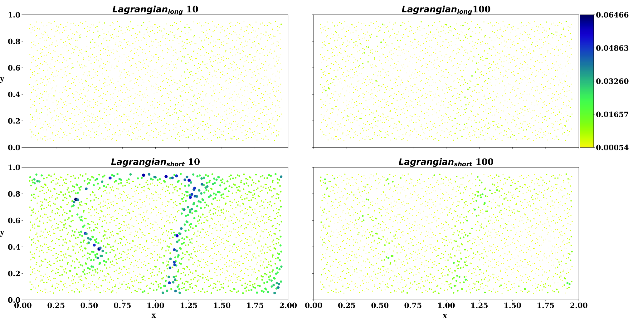

To understand the performance of our model with varying file cycle intervals, we evaluated four intervals, 10, 20, 50, and 100, in our experiments. We considered a total of 1,000 cycles of the Double Gyre data set. Further, we used a fixed number of 10,000 seeds to generate the training data sets.
In Figure 9, we report the error maps as well as the FTLE derived from using various configurations for training data generation. The was not impacted by the file cycle interval since each interpolation was independent of prior locations stored along the trajectory. Reconstruction of new trajectories using the model trained by the data involved an interpolation process where each location along the trajectory was dependent on the previous location. Thus, we observed a higher reconstruction error when the interval was short, and more intervals need to be spanned to construct a trajectory over the entire temporal duration. For example, for training data generated by the using an interval of 10, we saw the reconstruction error was higher for particles originating near FTLE ridges. These findings are consistent with the error analysis of Lagrangian-based particle tracing systems (9). Similar to prior experiments, in Figure 2(b), we observed the derived FTLE scalar fields are accurate for the , but contained some artifacts for the . Here, as expected, the shows fewer artifacts when using a longer file cycle interval.
Considering the violin plots in Figure 10, we obsersed varying reconstruction accuracy patterns. The accuracy did not change significantly with the file cycle interval. The local error of the was low for short intervals, but increased as the interval length increased due to greater divergence between neighboring trajectories over longer integration times. The global error of the represented the accuracy of particle trajectories that are “stitched”. We found the global error was the highest when the file cycle interval was short given a greater number of “stitching” events were involved. As the file cycle interval increased, although the accuracy of every individual interpolation (local error) was higher, the global error decreased due to fewer total interpolation steps. Again, these findings are consistent with prior work by 9 and 50. Additionally, we present the average error across all particles over time for the and approaches in Figure 11. The line curves provide strong evidence of local error propagation and accumulation for tests using training data.

For a qualitative assessment of the impact of the file cycle interval, we present reconstructed pathlines alongside the ground truth in Figure 12. We used piecewise linear interpolation to connect every interpolated location along the new trajectories. Although the demonstrated a small deviation from the ground truth when short file cycle intervals were used, the overall accuracy of reconstructed trajectories was high with interpolated results closely overlapping the ground truth.
4.6 Application to Fluid Dynamics Machine Learning Data Set

We applied our method to an ensemble member (#200) of the 2D fluid dynamics machine learning data set generated using the Gerris flow solver (31). The resolution of the original data set is . To generate the training data set, we placed seeds in the domain, set the file cycle interval to 10, and traced flow maps over the first 100 cycles. For particle advection, we used the VTK-m (40) library and a fourth-order Runge-Kutta (RK4) advection kernal. The median error of using our method after 100 cycles and 10 interpolation steps is approximately two times the grid cell size. Our method cost 0.6 seconds for reconstructing 2,000 particle trajectories using parallel inferences with OpenMP (11). When considering the storage requirements, the subset of the original data size we consider is approximately 209MB. Since our model has a fixed memory requirement, once trained, the storage costs are still fixed at 10.5 MB. To qualitatively evaluate the reconstructed data, we visualize pathlines inferred by the trained model in comparison with the ground truth in Figure 13. In future works, we aim to study how to improve inteprolation accuracy as well as determine an appropriate number of samples to be computed using in situ processing.
5 Future Work and Conclusion
Exploratory flow visualization for large-scale time-varying vector field data is challenging. In this paper, we introduced a deep neural network-based approach using Lagrangian represesntations to enable exploratory analysis. Our study demonstrated our model can be trained using Lagrangian representations extracted from a 2D time-varying vector field. Specifically, we used the widely studied unsteady Double Gyre analytical flow data set and one fluid dynamics machine learning data set to demonstrate our method. We contributed the first assessment of applying deep learning to various forms of Lagrangian representations and evaluated the efficacy of exploratory analysis. A benefit of using our method is the fixed memory required by a model and fast inference of unstructured spatiotemporal data. Our trained model requires only 10.5 MB, and consequently, time spent on I/O to load the model during post hoc analysis is negligible. Further, we are able to infer the pathlines of thousands of particles at interactive rates. With respect to reconstruction interpolation error, we found inference errors are small and follow predictable patterns consistent with results from prior works. Predictable and consistent error patterns enable effective future navigation of strategies to reduce reconstruction interpolation error when using machine learning. Overall, our study demonstrates the benefits of leveraging deep learning for exploratory flow visualization of time-varying vector field data.
An important direction for future work is investigating model performance for more complex or turbulent flows as well as large-scale 3D flow fields. With the objectives of improving spatial and temporal interpolation accuracy and reducing model training time, various forms of training data to train a model or different network architectures could be considered. For example, concatenate sets of trajectories to limit instances of error propagation while simultaneously accounting for reduced interpolation error due to stretching or divergence in the flow. Lastly, an open-source interactive tool for interactive flow visualization exploration, with a trained model serving as a backend, would be valuable to the community. We plan to pursue these projects in the future.
Acknowledgements.
The authors acknowledge current research support provided in part by the Intel Graphics and Visualization Institutes of XeLLENCE, the National Institutes of Health under grant numbers P41 GM103545 and R24 GM136986, the Department of Energy under grant number DE- FE0031880, and the Utah Office of Energy Development.References
- Red (2019)
Learning Rate Scheduler, , 2019.
URL https://pytorch.org/docs/stable/generated/torch.optim.lr_scheduler.ReduceLROnPlateau.html - Agranovsky et al. (2014) Agranovsky, A., Camp, D., Garth, C., Bethel, E.W., Joy, K.I., and Childs, H., Improved Post Hoc Flow Analysis Via Lagrangian Representations, 4th IEEE Symposium on Large Data Analysis and Visualization, LDAV, 2014.
- Agranovsky et al. (2015) Agranovsky, A., Obermaier, H., Garth, C., and Joy, K.I., A Multi-Resolution Interpolation Scheme for Pathline Based Lagrangian Flow Representations, Visualization and Data Analysis 2015, 2015.
- Ba et al. (2016) Ba, J.L., Kiros, J.R., and Hinton, G.E., Layer Normalization, arXiv preprint arXiv:1607.06450, 2016.
- Bai et al. (2019) Bai, X., Wang, C., and Li, C., A Streampath-Based RCNN Approach to Ocean Eddy Detection, IEEE Access, 2019.
- Berger et al. (2018) Berger, M., Li, J., and Levine, J.A., A Generative Model for Volume Rendering, IEEE transactions on visualization and computer graphics, 2018.
- Brunton et al. (2020) Brunton, S.L., Noack, B.R., and Koumoutsakos, P., Machine Learning for Fluid Mechanics, Annual Review of Fluid Mechanics, 2020.
- Bujack and Joy (2015) Bujack, R. and Joy, K.I., Lagrangian Representations of Flow Fields with Parameter Curves, IEEE Symposium on Large Data Analysis and Visualization (LDAV), 2015.
- Chandler et al. (2016) Chandler, J., Bujack, R., and Joy, K.I., Analysis of Error in Interpolation-Based Pathline Tracing, Proceedings of the Eurographics/IEEE VGTC Conference on Visualization: Short Papers, 2016.
- Chandler et al. (2015) Chandler, J., Obermaier, H., and Joy, K.I., Interpolation-Based Pathline Tracing in Particle-Based Flow Visualization, IEEE Transactions on Visualization and Computer Graphics, 2015.
- Dagum and Menon (1998) Dagum, L. and Menon, R., OpenMP: An Industry Standard API for Shared-Memory Programming, IEEE computational science and engineering, 1998.
- Deng et al. (2019) Deng, L., Wang, Y., Liu, Y., Wang, F., Li, S., and Liu, J., A CNN-based Vortex Identification Method, Journal of Visualization, 2019.
- Dong et al. (2015) Dong, C., Loy, C.C., He, K., and Tang, X., Image Super-Resolution Using Deep Convolutional Networks, IEEE transactions on pattern analysis and machine intelligence, 2015.
- Duo et al. (2019) Duo, Z., Wang, W., and Wang, H., Oceanic Mesoscale Eddy Detection Method Based on Deep Learning, Remote Sensing, 2019.
- Engel and Ropinski (2020) Engel, D. and Ropinski, T., Deep Volumetric Ambient Occlusion, IEEE Transactions on Visualization and Computer Graphics, 2020.
- Froyland and Junge (2018) Froyland, G. and Junge, O., Robust FEM-Based Extraction of Finite-Time Coherent Sets Using Scattered, Sparse, and Incomplete Trajectories, SIAM Journal on Applied Dynamical Systems, 2018.
- Froyland and Padberg-Gehle (2015) Froyland, G. and Padberg-Gehle, K., A rough-and-ready cluster-based approach for extracting finite-time coherent sets from sparse and incomplete trajectory data, Chaos: An Interdisciplinary Journal of Nonlinear Science, 2015.
- Garth et al. (2007) Garth, C., Gerhardt, F., Tricoche, X., and Hans, H., Efficient Computation and Visualization of Coherent Structures in Fluid Flow Applications, IEEE Transactions on Visualization and Computer Graphics, 2007.
- Guo et al. (2020) Guo, L., Ye, S., Han, J., Zheng, H., Gao, H., Chen, D.Z., Wang, J.X., and Wang, C., SSR-VFD: Spatial Super-Resolution for Vector Field Data Analysis and Visualization, 2020 IEEE Pacific Visualization Symposium (PacificVis), 2020.
- Hadjighasem et al. (2017) Hadjighasem, A., Farazmand, M., Blazevski, D., Froyland, G., and Haller, G., A Critical Comparison of Lagrangian Methods for Coherent Structure Detection, Chaos: An Interdisciplinary Journal of Nonlinear Science, 2017.
- Han et al. (2018) Han, J., Tao, J., and Wang, C., FlowNet: A Deep Learning Framework for Clustering and Selection of Streamlines and Stream Surfaces, IEEE Transactions on Visualization and Computer Graphics, 2018.
- Han et al. (2019) Han, J., Tao, J., Zheng, H., Guo, H., Chen, D.Z., and Wang, C., Flow Field Reduction Via Reconstructing Vector Data From 3-D Streamlines Using Deep Learning, IEEE computer graphics and applications, 2019.
- Han and Wang (2019) Han, J. and Wang, C., TSR-TVD: Temporal Super-Resolution for Time-Varying Data Analysis and Visualization, IEEE transactions on visualization and computer graphics, 2019.
- Han et al. (2020) Han, J., Zheng, H., Xing, Y., Chen, D.Z., and Wang, C., V2V: A Deep Learning Approach to Variable-to-Variable Selection and Translation for Multivariate Time-Varying Data, IEEE Transactions on Visualization and Computer Graphics, 2020.
- He et al. (2019) He, W., Wang, J., Guo, H., Wang, K.C., Shen, H.W., Raj, M., Nashed, Y.S., and Peterka, T., InSituNet: Deep Image Synthesis for Parameter Space Exploration of Ensemble Simulations, IEEE Transactions on Visualization and Computer Graphics, 2019.
- Hlawatsch et al. (2011) Hlawatsch, M., Sadlo, F., and Weiskopf, D., Hierarchical Line Integration, IEEE Transactions on Visualization and Computer Graphics, 2011.
- Hong et al. (2019) Hong, F., Liu, C., and Yuan, X., DNN-VolVis: Interactive Volume Visualization Supported by Deep Neural Network, 2019 IEEE Pacific Visualization Symposium (PacificVis), 2019.
- Hong et al. (2018) Hong, F., Zhang, J., and Yuan, X., Access Pattern Learning with Long Short-Term Memory for Parallel Particle Tracing, 2018 IEEE Pacific Visualization Symposium (PacificVis), IEEE, 2018.
- Hummel et al. (2016) Hummel, M., Bujack, R., Joy, K.I., and Garth, C., Error Estimates for Lagrangian Flow Field Representations, Proceedings of the Eurographics/IEEE VGTC Conference on Visualization: Short Papers, 2016.
- Intel (2007)
Intel, Intel Threading Building Blocks, , 2007.
URL https://www.intel.com/content/www/us/en/develop/tools/oneapi/components/onetbb.html - Jakob et al. (2020) Jakob, J., Gross, M., and Gunther, T., A Fluid Flow Data Set for Machine Learning and its Application to Neural Flow Map Interpolation, IEEE Transactions on Visualization and Computer Graphics, 2020.
- Kim et al. (2019) Kim, B., Azevedo, V.C., Thuerey, N., Kim, T., Gross, M., and Solenthaler, B., Deep Fluids: A Generative Network for Parameterized Fluid Simulations, Computer Graphics Forum, 2019.
- Kim and Günther (2019) Kim, B. and Günther, T., Robust Reference Frame Extraction from Unsteady 2D Vector Fields with Convolutional Neural Networks, Computer Graphics Forum, 2019.
- Kingma and Ba (2014) Kingma, D.P. and Ba, J., Adam: A Method for Stochastic Optimization, arXiv preprint arXiv:1412.6980, 2014.
- Lee and Park (2021) Lee, J.Y. and Park, J., Deep Regression Network-Assisted Efficient Streamline Generation Method, IEEE Access, 2021.
- Leventhal et al. (2019) Leventhal, S., Kim, M., and Pugmire, D., PAVE: An In Situ Framework for Scientific Visualization and Machine Learning Coupling, 2019 IEEE/ACM 5th International Workshop on Data Analysis and Reduction for Big Scientific Data (DRBSD-5), 2019.
- Lguensat et al. (2018) Lguensat, R., Sun, M., Fablet, R., Tandeo, P., Mason, E., and Chen, G., EddyNet: A Deep Neural Network for Pixel-Wise Classification of Oceanic Eddies, IGARSS 2018-2018 IEEE International Geoscience and Remote Sensing Symposium, 2018.
- Li et al. (2015) Li, Y., Wang, C., and Shene, C.K., Extracting Flow Features via Supervised Streamline Segmentation, Computers & Graphics, 2015.
- Liu et al. (2019) Liu, Y., Lu, Y., Wang, Y., Sun, D., Deng, L., Wang, F., and Lei, Y., A CNN-based shock detection method in flow visualization, Computers & Fluids, 2019.
- Moreland et al. (2016) Moreland, K., Sewell, C., Usher, W., Lo, L.t., Meredith, J., Pugmire, D., Kress, J., Schroots, H., Ma, K.L., Childs, H., , VTK-m: Accelerating the Visualization Toolkit for Massively Threaded Architectures, IEEE computer graphics and applications, 2016.
- Nair and Hinton (2010) Nair, V. and Hinton, G.E., Rectified Linear Units Improve Restricted Boltzmann Machines, Icml, 2010.
- Nardini et al. (2017) Nardini, P., Böttinger, M., Scheuermann, G., and Schmidt, M., Visual study of the benguela upwelling system using pathline predicates, Workshop on Visualisation in Environmental Sciences (EnvirVis), 2017.
- Paszke et al. (2019) Paszke, A., Gross, S., Massa, F., Lerer, A., Bradbury, J., Chanan, G., Killeen, T., Lin, Z., Gimelshein, N., Antiga, L., Desmaison, A., Kopf, A., Yang, E., DeVito, Z., Raison, M., Tejani, A., Chilamkurthy, S., Steiner, B., Fang, L., Bai, J., and Chintala, S., 2019. PyTorch: An Imperative Style, High-Performance Deep Learning Library. Advances in Neural Information Processing Systems 32.
- Qin et al. (2014) Qin, X., van Sebille, E., and Sen Gupta, A., Quantification of errors induced by temporal resolution on Lagrangian particles in an eddy-resolving model, Ocean Modelling, 2014.
- Rapp et al. (2019) Rapp, T., Peters, C., and Dachsbacher, C., Void-and-Cluster Sampling of Large Scattered Data and Trajectories, IEEE Transactions on Visualization and Computer Graphics, 2019.
- Rockwood et al. (2019) Rockwood, M.P., Loiselle, T., and Green, M.A., Practical concerns of implementing a finite-time lyapunov exponent analysis with under-resolved data, Experiments in Fluids, 2019.
- Sahoo and Berger (2021) Sahoo, S. and Berger, M., Integration-Aware Vector Field Super Resolution, 2021.
- Sane et al. (2018) Sane, S., Bujack, R., and Childs, H., Revisiting the Evaluation of In Situ Lagrangian Analysis, EGPGV@ EuroVis, 2018.
- Sane et al. (2020) Sane, S., Bujack, R., Garth, C., and Childs, H., A Survey of Seed Placement and Streamline Selection Techniques, Computer Graphics Forum, Wiley Online Library, 2020.
- Sane et al. (2019) Sane, S., Childs, H., and Bujack, R., An Interpolation Scheme for VDVP Lagrangian Basis Flows, Eurographics Symposium on Parallel Graphics and Visualization, 2019.
- Sane et al. (2021a) Sane, S., Johnson, C.R., and Childs, H., Investigating In Situ Reduction via Lagrangian Representations for Cosmology and Seismology Applications, International Conference on Computational Science, 2021a.
- Sane et al. (2021b) Sane, S., Yenpure, A., Bujack, R., Larsen, M., Moreland, K., Garth, C., Johnson, C.R., and Childs, H., Scalable In Situ Computation of Lagrangian Representations via Local Flow Maps, 2021b.
- Schlueter-Kuck and Dabiri (2017) Schlueter-Kuck, K.L. and Dabiri, J.O., Coherent structure colouring: identification of coherent structures from sparse data using graph theory, Journal of Fluid Mechanics, 2017.
- Shadden et al. (2005) Shadden, S.C., Lekien, F., and Marsden, J.E., Definition and properties of Lagrangian coherent structures from finite-time Lyapunov exponents in two-dimensional aperiodic flows, Physica D: Nonlinear Phenomena, 2005.
- Shi et al. (2016) Shi, W., Caballero, J., Huszár, F., Totz, J., Aitken, A.P., Bishop, R., Rueckert, D., and Wang, Z., Real-Time Single Image and Video Super-Resolution Using an Efficient Sub-Pixel Convolutional Neural Network, Proceedings of the IEEE conference on computer vision and pattern recognition, 2016.
- Siegfried et al. (2019) Siegfried, L., Schmidt, M., Mohrholz, V., Pogrzeba, H., Nardini, P., Böttinger, M., and Scheuermann, G., The tropical-subtropical coupling in the southeast atlantic from the perspective of the northern benguela upwelling system, PloS one, 2019.
- Ströfer et al. (2018) Ströfer, C.M., Wu, J., Xiao, H., and Paterson, E., Data-Driven, Physics-Based Feature Extraction from Fluid Flow Fields Using Convolutional Neural Networks, Communications in Computational Physics, 2018.
- Valdivieso Da Costa and Blanke (2004) Valdivieso Da Costa, M. and Blanke, B., Lagrangian methods for flow climatologies and trajectory error assessment, Ocean Modelling, 2004.
- van Sebille et al. (2018) van Sebille, E. , Lagrangian ocean analysis: Fundamentals and practices, Ocean Modelling, 2018.
- Wang et al. (2021) Wang, Y., Deng, L., Yang, Z., Zhao, D., and Wang, F., A Rapid Vortex Identification Method Using Fully Convolutional Segmentation Network, The Visual Computer, 2021.
- Weiss et al. (2019) Weiss, S., Chu, M., Thuerey, N., and Westermann, R., Volumetric Isosurface Rendering with Deep Learning-Based Super-Resolution, IEEE transactions on visualization and computer graphics, 2019.
- Yi (2018) Yi, T.B.L., CNN-based Flow Field Feature Visualization Method, International Journal of Performability Engineering, 2018.