Rapid-cycle Thouless pumping in a one-dimensional optical latticePreprint: APS/123-QED

The past few decades have been marked by the discovery of various systems where topological properties of the quasiparticle spectrum are connected with the quantization of particle transport, for example Thouless pumping Thouless 1983 or the integer quantum Hall effect Thouless et al. 1982; Niu and Thouless 1984. In Thouless pumping, this integer valued particle transport is achieved by performing a non-contractible adiabatic loop through a non-degenerate parameter space. The amount of pumped charge can then be expressed by the Chern number associated with the Berry or Zak phase Berry 1984; Zak 1989; Xiao et al. 2010. Although the original mathematics of the Thouless pumping dates back 30 years, the effect has only recently been observed directly using ultracold bosonic atoms in an optical superlattice Lohse et al. 2015; Nakajima et al. 2016.

The adiabacity of the non-contractible loop is required to ensure the topological robustness of the Thouless pump. Generally, corrections to the quantization of particle transport arise when the parameter space is traversed at a finite frequency Wang et al. 2013; Privitera et al. 2018. For special cases of Thouless pumping, such as parametric pumps Switkes et al. 1999; Brouwer 1998; Altshuler and Glazman 1999; Levinson et al. 2001; Entin-Wohlman et al. 2002, these non-adiabatic effects were studied Wang et al. 2013; Privitera et al. 2018; Ohkubo 2008a; Ohkubo 2008b; Cavaliere et al. 2009; Uchiyama 2014; Watanabe and Hayakawa 2014. In order to minimise corrections, strategies such as dissipation assisted pumping Arceci et al. 2020, non-Hermitian Floquet engineering Höckendorf et al. 2020; Fedorova et al. 2020 and adiabatic shortcuts by external control Takahashi et al. 2020; Funo et al. 2020 were proposed. Recently however, a family of finite-frequency protocols on the Rice-Mele insulator have been constructed, in which all the quasi-excitations disappear altogether at the end of a rapid-cycle, resulting in a perfectly quantized and noise-free particle transport outside of the adiabatic limit Malikis and Cheianov 2021. Although this resolves the issue of non-adiabatic breaking of topological quantization in an ideal homogeneous system, there might still be finite-size corrections Li and Fleischhauer 2017 or corrections due to perturbations in the insulator, such as inhomogeneity due to an external potential. Understanding of such corrections is important in the context of experimental realization of the rapid cycle pump, for example, in an ultracold atomic system.

In this paper, starting from the Rice-Mele insulator as the zeroth-order approximation, we investigate the corrections in the expectation value of the pumped charge w.r.t quantization due to performing a rapid-cycle protocol inside a one-dimensional optical lattice. Specifically, we investigate finite-size corrections, introduce next-to-nearest neighbour hopping and add a weak harmonic potential to the system. A lattice variant of the Weyl transform Case 2008 is constructed to retrieve analytical relations between the corrections and the potential curvature. It is shown that all the corrections decay exponentially with the protocol defining parameters, which could also be chosen such that the corrections vanish completely. Lastly, a discussion is given on the change of center of mass after a rapid pumping cycle. It is shown that the corrections due to the rapid-cycle protocol under the harmonic potential are most pronounced in the change in center of mass, which is the current proposed and used method of measuring the charge pump Wang et al. 2013; Lohse et al. 2015; Nakajima et al. 2016.

We begin with a recapitulation on the Rice-Mele model Rice and Mele 1982. This is a tight binding chain consisting of $2N$ atoms, on which there are orthonormal positional state $|\alpha\rangle$ which are subject to periodic boundary conditions, i.e. $|\alpha+2N\rangle=|\alpha\rangle$. In the single-particle subspace, the Hamiltonian of this model is given by

$$\begin{split}\hat{H}_{RM}(p)=&\sum_{\alpha=0}^{N-1}\bigg[m\Big(|2\alpha\rangle\langle 2\alpha|-|2\alpha+1\rangle\langle 2\alpha+1|\Big)\\ &+\Big(t_{1}|2\alpha\rangle\langle 2\alpha+1|+t_{2}|2\alpha-1\rangle\langle 2\alpha|+h.c.\Big)\bigg],\end{split}$$

(1)

where $p=(m,t_{1},t_{2})$ are the tight-binding parameters. A graphical representation of this model is shown in Fig. 1. The periodicity ensures that the Hamiltonian (1) can be written in the reciprocal space

$$\hat{H}_{RM}(k,p):=\begin{bmatrix}m&t_{1}e^{\frac{ik}{2}}+t_{2}^{*}e^{-\frac{ik}{2}}\\ t_{1}^{*}e^{-\frac{ik}{2}}+t_{2}e^{\frac{ik}{2}}&-m\end{bmatrix},$$

(2)

where $k\in\mathscr{B}=\left\{-\pi+m\frac{2\pi}{N}\mid 0\leq m<N\right\}$, the discretised Brillouin zone. This Hamiltonian has two quasienergies $\epsilon_{\pm}(k,p)$ with the property $\epsilon_{-}(k,p)=-|\epsilon_{+}(k,p)|$. This creates two distinct energy bands which are seperated by the energy gap $E_{gap}=2\sqrt{m^{2}+\delta^{2}}$, where $\delta=|t_{1}|-|t_{2}|$. If we consider the parameter space $\mathscr{P}=\{(m,t_{1},t_{2})\mid E_{gap}>0\}$ where this energy gap is strictly positive, then this space has a non-trivial fundamental group. Considering a non-contractible loop $p:[0,T)\rightarrow\mathscr{P}$ through this parameter space, we can look at the evolution of the lower energy Bloch states $|u_{-}(k,\tau)\rangle$ according to the Schrödinger equation

$$\begin{split}i\frac{d}{d\tau}|u_{-}(k,\tau)\rangle=\hat{H}_{RM}(k,p(\tau))|u_{-}(k,\tau)\rangle\text{ with}\\ \hat{H}_{RM}(k,p(0))|u_{-}(k,0)\rangle=\epsilon_{-}(k,p(0))|u_{-}(k,0)\rangle.\end{split}$$

(3)

If the path through the parameter space is adiabatic, i.e. infinitely slowely, the Bloch states are ensured to be the lower eigenstates of the instantaneous Hamiltonian at all times and therefore no excitations will occur Born and Fock 1928. It can be shown that in the thermodynamic limit $N\rightarrow\infty$, the non-contractibility of the loop through the parameter space will then result in a non-zero pumped charge which is equal to the winding number of this loop around the degeneracy point Xiao et al. 2010. This pumped charge can be directly related to the first Chern number associated with the Berry connection form Xiao et al. 2010; Berry 1984.

Outside of the adiabatic limit, i.e. at finite frequencies, there is generally a correction to this integer valued pumped charge Privitera et al. 2018. Recently however, a family of protocols were constructed which results in noise-free integer valued Thouless pumping at finite frequencies Malikis and Cheianov 2021. Here, we investigate one such protocol. Consider the space $\{(x,y)\}=\mathbb{R}^{2}$ and a real oscillating function $\phi(y)$ which is a solution to

$$\partial_{y}^{2}\phi+\sinh\phi=0.$$

(4)

The integrated form of this differential equation is given by

$$(\partial_{y}\phi)^{2}+2\cosh\phi=2\varepsilon,$$

(5)

where $\varepsilon\in\mathbb{R}_{>0}$ and the period of $\phi$ will be denoted by $T_{\phi}(\epsilon)$. As the initial condition, we will choose $\phi(0)=0$. It can be shown that this differential equation is equivalent to the zero curvature condition

$$\partial_{y}\hat{A}_{x}-\partial_{x}\hat{A}_{y}+\left[\hat{A}_{x},\hat{A}_{y}\right]=0$$

(6)

for the anti-Hermitian matrix-valued vector fields

	$\displaystyle\hat{A}_{x}$	$\displaystyle=\frac{1}{4}\begin{bmatrix}i\partial_{y}\phi&2\cosh\left(\frac{\phi-ik}{2}\right)\\ -2\cosh\left(\frac{\phi+ik}{2}\right)&-i\partial_{y}\phi\end{bmatrix}$		(7)
	$\displaystyle\hat{A}_{y}$	$\displaystyle=\frac{i}{4}\begin{bmatrix}0&2\sinh\left(\frac{\phi-ik}{2}\right)\\ 2\sinh\left(\frac{\phi+ik}{2}\right)&0\end{bmatrix}$		(8)

where $k$ is a real valued parameter. The zero curvavature condition (6) implies the existence of two orthonormal globally well-defined solutions $|F_{\pm}\rangle\in\mathbb{C}^{2}$ of the system of equations

$$\partial_{x}|F_{\pm}\rangle=\hat{A}_{x}|F_{\pm}\rangle,\quad\partial_{y}|F_{\pm}\rangle=\hat{A}_{y}|F_{\pm}\rangle.$$

(9)

It should be noted that $|F_{\pm}\rangle$ depends on $x,y$ and $k$, which we will not write this down explicitly in the rest of this paper. Let $b\in\mathbb{R}$, $T=\frac{2\pi}{b}$ and the differentiable path $\gamma\colon\left[0,T\right]\rightarrow\mathbb{R}^{2}$ given by

$$\gamma_{x}(\tau)=\tau,\quad\gamma_{y}(\tau)=\frac{T_{\phi}(\epsilon)}{2\pi}\left[b\tau-\sin(b\tau)\right],$$

(10)

then we can define the matrix

$$\hat{H}_{\gamma}(k,\tau)=i\dot{\gamma}_{x}\hat{A}_{x}+i\dot{\gamma}_{y}\hat{A}_{y}$$

(11)

which coincides with the Rice-Mele Hamiltonian in reciprocal space (2). The solutions of the system of equations (9) will now evolve along the path $\gamma$ according to the Schrödinger equation

$$i\frac{d}{d\tau}|F_{\pm}\rangle=\hat{H}_{\gamma}|F_{\pm}\rangle.$$

(12)

Furthermore, since $\dot{\gamma}_{y}(0)=\dot{\gamma}_{y}\left(T\right)=0$, the solutions $|F_{\pm}\rangle$ at $\tau=0$ and at $\tau=T$ are the eigenstates of $\hat{H}_{\gamma}$, where we choose $|F_{-}\rangle$ to correspond to the lower eigenvalue. This protocol will result in a non-contractible loop in $\mathscr{P}$, such that the energy gap remains positive. This energy gap does however change during the evolution. Therefore, we will consider the function

$$s(\tau)=\int_{0}^{\tau}d\tau^{\prime}\ E_{gap}(\tau^{\prime})$$

and reparametrize the path $\gamma$ in Eq. (10) by

$$\gamma(\tau)\mapsto\gamma\left(s^{-1}(\tau)\right)\text{ and }T\mapsto s(T)$$

(13)

such that $E_{gap}=1$ at all times. The non-contractibility of the loop in $\mathscr{P}$ and the fact that $|F_{-}\rangle$ is an eigenstate of the Hamiltonian at the start and end of the protocol will now result in a non-zero integer valued particle transport in the thermodynamic limit Malikis and Cheianov 2021.

Since this protocol works at finite frequencies, there are excitations of quasiparticles during the evolution. However, it makes sure that all of these excitations vanish at the end, such that the result after a rapid cycle is the exact same as with an adiabatic cycle. This is true for all values of $b$ and $\varepsilon$, which are the only two parameters the protocol depends on. The parameter $\varepsilon$ determines the width of the valence band and the conduction band. i.e.

$$\max\{|\epsilon_{\pm}(k)|\}-\min\{|\epsilon_{\pm}(k))|\}=\frac{1}{2}\left[\sqrt{\frac{\varepsilon+1}{\varepsilon-1}}-1\right],$$

(14)

where it can be seen that the width of the bands becomes infinitely large in the limit $\varepsilon\downarrow 1$ and vanishes in the limit $\varepsilon\rightarrow\infty$. The parameter $b$ determines the steepness and therefore the period of the path $\gamma$ as in Eq. (10). A larger value for $b$ will also result in a more rapid pumping cycle. One should note that the angular frequency is in fact a function of both $b$ and $\varepsilon$, since the reparametrization (13) depends on $\varepsilon$. In the rest of this paper, we will investigate this specific protocol. It should be noted that other protocols could result in different specific properties. It is however expected that the general properties are similar for all rapid-cycle protocols.

The proposed protocol gives a quantized particle transport outside of the adiabatic limit, but still only works in the thermodynamic limit. There are in general corrections to the pumped charge which decrease exponentially with $N$ Li and Fleischhauer 2017. Here, we will investigate those corrections for the rapid-cycle protocol specifically. If we consider the pumped charge per $k$-number, then because of its periodicity in $k$, it can be written as a Fourier series, i.e.

$$\Delta Q(k):=\int_{0}^{T}\langle F_{-}|\partial_{k}\hat{H}_{\gamma}|F_{-}\rangle d\tau=\sum_{n=-\infty}^{\infty}\Delta Q_{n}e^{ink},$$

(15)

where $\Delta Q_{n}$ are the Fourier coefficients. In systems with a size $N\in\mathbb{N}$, the total pumped charge becomes

$$\Delta Q:=\frac{1}{N}\sum_{k\in\mathscr{B}}\Delta Q(k)=\Delta Q_{0}+\sum_{m=1}^{\infty}\Delta Q_{mN}+\Delta Q_{-mN},$$

(16)

which reduces to $\Delta Q=\Delta Q_{0}\in\mathbb{Z}$ in the limit $N\rightarrow\infty$. Therefore, in finite-sized systems, the corrections are due to the additional Fourier-coefficients. Note that these finite sized corrections vanish if for all $n\in\mathbb{N}$, we have $\Delta Q_{n}=-\Delta Q_{-n}$ or $\Delta Q_{n}=\Delta Q_{-n}=0$. It might be possible to construct a protocol in which this is true. In general however, this is not the case and there are still finite-sized correction. In the discussed rapid-cycle protocol, there is an analytical expression for the pumped charge per $k$-number. Namely, the pumped charge after one cycle due to the state $|F_{-}\rangle$ can be derived to be

$$\begin{split}\Delta Q(k)=-\frac{1}{2}\int_{0}^{T_{\phi}(\epsilon)}\frac{\cosh(\phi(y))+\cos(2k)}{\sqrt{2\epsilon+2\cos(2k)}}dy.\end{split}$$

(17)

Note that this is an even function, such that $\Delta Q_{-n}=\Delta Q_{n}$. Furthermore, it can be demonstrated that in the limit $\varepsilon\gg 1$ we get that $\Delta Q_{n}\ll 1$ for all $n\geq 2$. So in the limit where the width of the bands vanishes and the dispersion relation becomes flat, all finite-size corrections vanish for systems with $N\geq 2$. In Fig. 2(a), the Fourier coefficients have been plotted for different values of $\varepsilon$. It can indeed be seen that in the limit $\varepsilon\gg 1$, most Fourier coefficients are negligible. In Fig. 2(b), the finite size corrections are shown as function of $N$. It can be seen that as both $\varepsilon$ and $N$ increase, the finite sized correction start to vanish and become negligible w.r.t the numerical errors. Therefore, even for small systems it is possible to have a close to integer valued rapid-cycle Thouless pumping, where the corrections are actually independent on the rapidity.

Thouless pumping can be realized experimentally in a double-well optical superlattice of the form

$$V(x,\tau)=-V_{S}(\tau)\cos^{2}\left(\frac{2\pi x}{d}\right)-V_{L}(\tau)\cos^{2}\left(\frac{\pi x}{d}-\phi(\tau)\right),$$

(18)

where $d$ is the lattice constant, $V_{s}$ and $V_{L}$ the depth of the short and long lattice respectively and $\phi$ the phase difference between the two lattices Wang et al. 2013; Lohse et al. 2015; Nakajima et al. 2016; Peil et al. 2003; Qian et al. 2011. In the discussion of this lattice, we will use the unit of energy to be the recoil energy $E_{R}:=\hbar^{2}/(8md^{2})$, where $m$ is the mass of the used atom. In the deep tight-binding limit, the two lowest energy bands of this model (18) can be approximated by those of the RM-Hamiltonian (1). Generally however, there is a slight difference between these two models. The band structure of the optical lattice can then be fully captured by considering higher hopping terms to the RM-Hamiltonian. Here, we will only consider the next-to-nearest-neighbour hopping terms, namely

$$\begin{split}\hat{H}_{NN}=&\sum_{\alpha=0}^{N-1}t_{3}|2\alpha\rangle\langle 2\alpha+2|+t_{4}|2\alpha-1\rangle\langle 2\alpha+1|+h.c.\end{split}$$

(19)

which is added to the RM-Hamiltonian. With the addition of the NN-hopping terms, the two lower bands of the optical lattice coincide with those in the tight-binding approximation in sufficiently deep lattices, where the energy gap is much larger than the width of the bands. These extra NN-hopping terms will in general result in a deviation in the pumped charge. Specifically, when $|t_{4}-t_{3}|\ll E_{gap}$, these corrections to integer values pumped charge are linearly dependent on the difference $|t_{4}-t_{3}|$. For the ease of calculation, we will assume that the NN-hopping terms stay constant during the protocol. Although this is not generally true, this does give an idea of the order of magnitude, or at least an upper bound of the corrections due to the additional terms. In the rapid-cycle protocol, the deviation from integer valued pumped charge after one cycle is calculated as function of $\varepsilon$ and $1/b$ and shown in Fig. 3. It can be seen that the corrections are oscillatory in $1/b$ and $\varepsilon$, which means there are lines where the corrections vanish completely. Moreover, the amplitude of these oscillations decrease exponentially with both $\varepsilon$ and $1/b$. This means that in the adiabatic limit $b\rightarrow 0$ and in the limit of a flat dispersion $\varepsilon\rightarrow\infty$ there are no corrections to integer valued pumped charge due to NN-hopping terms.

In order to calculate actual corrections, we should consider the magnitude of $|t_{4}-t_{3}|$ in the optical lattice (18). For simplicity however, we will only calculate the magnitude of the sum of the NN-hopping terms, i.e. $|t_{3}+t_{4}|$, since this sum can be easily calculated by making use of the fact that

$$\epsilon_{-}(k)+\epsilon_{+}(k)=2\cdot\text{Re}\left((t_{3}+t_{4})e^{ik}\right),$$

(20)

where $\epsilon_{\pm}(k)$ are the quasienergies of the RM-Hamiltonian with NN-hopping terms. In order to calculate the magnitude of the difference $|t_{4}-t_{3}|$, one would need some fitting procedure for the bands. It is however expected that the order of magnitude of the difference $|t_{4}-t_{3}|$ is similar to the order of magnitude of the sum $|t_{3}+t_{4}|$. In Fig. 4, the magnitude of the sum of the NN-hopping terms per energy gap is plotted against $V_{S}$ and $V_{L}$ where $\phi=0$. It can be seen that this magnitude decreases exponentially with both $V_{S}$ and $V_{L}$. Moreover, on the line $V_{S}=V_{L}^{2}/(16E_{R})$, the NN-hopping terms are maximal, and this region should therefore be avoided to keep the NN-hopping terms to a minimum. As $\phi$ is varied, the absolute NN-hopping terms do not change significantly, while the energy gap does change. This will result in the ratio between the hopping constants and the energygap to change during the protocol, which already shows that the assumption that the NN-hopping terms stay constant is not true. The parameters $V_{S}$ an $V_{L}$ could also be varied during the protocol to overcome this problem.

Although the rapid-cycle protocol removes the finite-frequency corrections of adiabatic cycles, the NN-hopping terms introduce new corrections, whereas the topological quantization is still ensured in adiabatic cycles. Therefore, the parameters of the optical lattice should be chosen to minimize the NN-hopping terms. Also, to get the full characteristics of the optical lattice, even higher hopping terms should be considered. These are however expected to be negligible w.r.t the NN-hopping terms. Since we have not computed the exact mapping of the whole rapid-cycle protocol onto the optical lattice, we have not actually calculated the exact corrections that would occur in an optical lattice experiment, where there are most certainly varying NN-hopping terms. However, one should expect the order of magnitude of the corrections to be similar.

In the optical lattice, the particles get trapped inside a harmonic potential, laid in the length of the lattice. In the single-particle subspace, this harmonic potential is given by

$$\hat{V}=\sum_{\alpha=0}^{N-1}\frac{1}{2}\xi\left(\alpha-\alpha_{0}\right)^{2}\Big(|2\alpha\rangle\langle 2\alpha|+|2\alpha+1\rangle\langle 2\alpha+1|\Big),$$

(21)

where $\xi\in\mathbb{R}_{>0}$ is analogous to the spring constant in a classical system, and $\alpha_{0}=\frac{N-1}{2}$ is the center of the lattice. We will from now on consider $N$ to be odd, such that there is actually a center unit cell where the added potential vanishes. This added potential has the effect of localizing the eigenstates of the total Hamiltonian $\hat{H}=\hat{H}_{RM}+\hat{V}$. Here, we do not consider the NN-hopping terms, suppose the potential is smooth with $\xi\ll 1$ and the size of the system $N$ is large enough such that for the states

$$\mathcal{S}=\{|\psi\rangle:\hat{H}|\psi\rangle=E|\psi\rangle\text{ and }E<0\},$$

(22)

the amplitude at the edges of the system become negligible. Here, $\mathcal{S}$ is the set of vacuum states in the zero temperature limit with a chemical potential $\mu=0$. Using the fact that the potential is weak and smooth, the lattice looks locally unperturbed and periodic. Therefore, the non-contractible loop through $\mathscr{P}$ using the rapid-cycle protocol will still result in a non-zero particle transport. This particle transport is also close to integer as shown in Fig. 5, with some corrections due to the harmonic potential. To get these corrections, we will analyse the system in the phase space by introducing a lattice variant of the Weyl transform Case 2008. Namely, we define the Weyl transform of an operator $\hat{A}$ by the $2\times 2$ matrix $\tilde{A}(n,k)$ given by

$$\begin{split}&\langle\alpha|\tilde{A}(n,k)|\beta\rangle=\\ &\sum_{x=0}^{N-1}e^{-ik\left(2x+\frac{\alpha-\beta}{2}\right)}\langle 2(n+x)+\alpha|\hat{A}|2(n-x)+\beta\rangle\end{split}$$

(23)

with $\alpha,\beta\in\{0,1\}$. More details and properties of this transformation are given in Appendix A. This Weyl transform can be applied to our system containing the Rice-Mele Hamiltonian (1) and the added harmonic potential (21), such that the Weyl transform of the Hamiltonian is given by

$$\tilde{H}(n,k)(\tau)=\hat{H}_{\gamma}(k,\tau)+\frac{1}{2}\xi n^{2}\mathbb{I}_{2},$$

(24)

which is the sum of the Rice-Mele Hamiltonian in reciprocal space (11) and a scalar matrix associated with the harmonic potential, translated such that the center of the lattice lies at $n=0$. The Weyl tansform therefore simplifies to a two dimensional problem, in which we consider the Weyl transformed Liouvile-von Neumann equation

$$i\frac{\partial\tilde{\rho}}{d\tau}=\widetilde{H\rho}-\widetilde{\rho H}.$$

(25)

As discussed in Appendix B, this gives rise to an expansion of the local vacuum density matrix in the insulating region, given by

$$\tilde{\rho}(n)=\tilde{\rho}_{0}+\xi\left(\tilde{\rho}_{1}+n\tilde{\rho}_{2}\right)+\xi^{2}\left(\tilde{\rho}_{3}+n\tilde{\rho}_{4}+n^{2}\tilde{\rho}_{5}\right)+\mathcal{O}\left(\xi^{3}\right),$$

(26)

where $\tilde{\rho}_{0}$ is the local density matrix of the unperturbed lattice and the subsequent terms are corrections due to the harmonic potential. Eq. (26) shows the general dependence of the density matrix on $n$ and $\xi$. Here, $\tilde{\rho}_{1}$ and $\tilde{\rho}_{4}$ are scalar matrices and also the only correction terms which have non-zero trace. This gives that in the limit $\varepsilon\gg 1$, the trace of the local density matrix is given by

$$\text{tr}(\tilde{\rho}(n))=1+\frac{1}{4\varepsilon}\left(\xi+3n\xi^{2}\right)+\mathcal{O}(\xi^{3})>1,$$

(27)

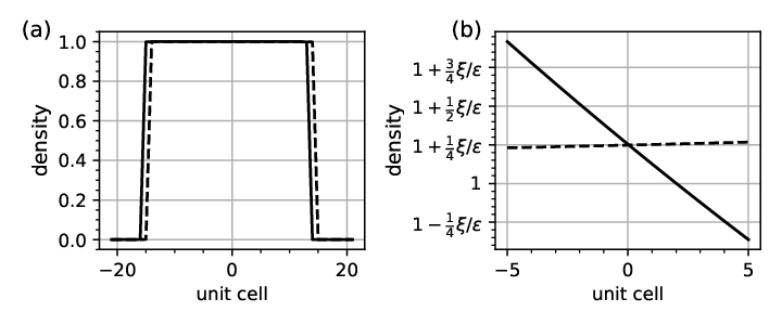
meaning that inside the insulating region, the amount of particles per unit cell is greater than one and there is a slight cross-over with the conduction band in the vacuum state which scales inversely proportional to $\varepsilon$, as shown in Fig. 8(b).

We are now interested in the corrections to the total pumped charge due to the harmonic potential. The expansion of the density matrix (26) gives the general dependence of the corrections in pumped charge on the position $n$ and the spring constant $\xi$. Here, it should be noted that $\tilde{\rho}_{1}$ and $\tilde{\rho}_{4}$ are scalar matrices and therefore have no contribution to the pumped charge. Moreover, since the position dependence is defined per unit cell, we have to distinguish between the current through a unit cell and between adjacent unit cells, as shown in Fig. 6. We can write the total pumped charge after one cycle through unit cell $n$ as

$$\begin{split}\Delta Q(n)-\Delta Q_{0}&=n\xi\big(A_{1}+B_{1}\big)\\ &+n^{2}\xi^{2}\big(A_{2}+B_{2}\big)\\ &+\xi^{2}\big(A_{3}+B_{3}\big)+\mathcal{O}(\xi^{3})\end{split}$$

(28)

and the pumped charge between unit cells $n$ and $n+1$ as

$$\begin{split}\Delta Q\left(n+\frac{1}{2}\right)-\Delta Q_{0}&=\left(n+\frac{1}{2}\right)\xi\big(A_{1}-B_{1}\big)\\ &+\left(n+\frac{1}{2}\right)^{2}\xi^{2}\big(A_{2}-B_{2}\big)\\ &+\xi^{2}\big(A_{3}-B_{3}\big)+\mathcal{O}(\xi^{3}),\end{split}$$

(29)

where $\Delta Q_{0}\in\mathbb{Z}$ is the unperturbed integer valued pumped charge and the terms $A_{i}$ and $B_{i}$ depend on the path through the parameter space, i.e. depend on $\varepsilon$ and $b$. Here, the $A_{i}$ terms can be thought of as the average pumped charge between each of the atoms, while the $B_{i}$ terms describe the polarization within the unit cells. In Fig. 7, the numerical calculations of these coefficients are shown. It can be seen that that the behaviour of these functions is oscillatory, with minima where the coefficients become exactly equal to 0. The amplitude of these functions decays exponentially with both $\varepsilon$ and $1/b$. The non-zero $B_{i}$ coefficients cause a polarization in each unit cell, resulting in a change in energy. In the limit $\varepsilon\gg 1$, it can be derived that the the change in local energy is given by

$$\begin{split}\Delta E(n)&=2n\xi B_{1}+n^{2}\xi^{2}\left(2B_{2}-\frac{1}{2}(A_{1}-B_{1})\right)\\ &+\xi^{2}\left(2B_{3}-\frac{1}{4}\left(A_{2}-B_{2}\right)\right)+\mathcal{O}(\xi^{3}).\end{split}$$

(30)

This shows that in the rapid-cycle protocol, local excitations start to appear due to the harmonic potential. Interestingly, it possible to have a local correction to the pumped charge, while the expectation value of the local energy does not change. This suggests that there is additional noise on the energy and pumped charge, which could be investigated in further research.

Similar to the addition of NN-hopping, we can see that the rapid-cycle protocol in a harmonic potential creates additional corrections to an integer valued charge pump, whereas an adiabatic protocol only has finite-frequency corrections Privitera et al. 2018; Lohse et al. 2015; Nakajima et al. 2016. At the center of the lattice, the corrections in a rapid-cycle scale with $\xi^{2}$, which makes them quite small for weak harmonic potentials, and could even be negligible w.r.t the correction due to NN-hopping in the optical lattice. When we go off-center, there are corrections which only scale linearly with $\xi$. However, since these corrections also scale linearly with $n$, the average pumped charge of a bulk around the center again scales quadratically with the potential curvature.

In the optical lattice experiment, it is not actually the pumped charge through a point which is measured, but rather the change in center of mass of the whole density distribution Wang et al. 2013; Lohse et al. 2015; Nakajima et al. 2016. As seen in Fig. 8(a), the density distribution, and therefore also the center of mass, shifts after a pumping cycle. This measurement technique makes use of the fact that the pumping is close to integer inside the whole insulating region. However, as seen in Eq. (28) and Eq. (29), the pumped charge inside the insulating region depends on the position. By the continuity equation, this will result in a change in density distribution inside the insulating region after a pumping cycle. In Fig. 8(b), this change in density distribution per unit cell is plotted after one cycle. Besides a change in density per unit cell, there is also the polarization of density in each unit cell. These two effects will result in a correction to the change in center of mass w.r.t integer value. Moreover, one should note that there are additional corrections due to the compressible region.

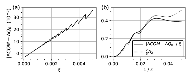
As discussed at the end of Section V, the average pumped charge in the bulk of the insulating region scales with $\xi^{2}$. It should be noted however, that the width of the insulating region also depends on $\xi$, and scales with $\xi^{-1/2}$. This will cause corrections to the change in center of mass to be linearly dependent on $\xi$. Specifically, using the continuity equation, Eq. (28) and Eq. (29), it can be demonstrated that the correction to the change in center of mass w.r.t integer value of the insulating region is given by

$$\left|\Delta_{\rm COM}-\Delta Q_{0}\right|\approx\frac{2}{3}\xi A_{2}+\mathcal{O}(\xi^{2})$$

(31)

in the limit $\varepsilon\gg 1$. In addition to the corrections due to the insulating region, the compressible region will also give some corrections. Although the compressible region is minimal in the same limit $\varepsilon\gg 1$, it does not vanish. In Fig. 9(a), it can be seen that the relation between the correction to the change in center of mass as function of $\xi$ is staggered. This can be explained by the fact that the width of both the insulating and compressible region is always integer valued. Therefore, a small variation in $\xi$ will not directly result in a variation in the width of the compressible region. When the variation in $\xi$ is large enough however, the compressible region will jump to the next atom, which causes the staggered behaviour. In Fig. 9(b), it can be seen that the Eq. (31) gives a good approximation for $\varepsilon\gg 1$, where there are some slight corrections due to the compressible region.

The finite-frequency corrections to the pumped charge in adiabatic cycles scale with $\omega^{2}$ Privitera et al. 2018 and the potential corrections in a rapid-cycle protocol scale with $\xi^{2}$. However, the corrections to the change in center of mass scale only linearly with $\xi$. The rapid-cycle protocol might therefore introduce more corrections to the center of mass method than the adiabatic cycle would have given. Moreover, using this method, one also needs to take the corrections to the pumped charge due to the compressible region into account. Therefore, one might want to consider other methods in order to directly measure the actual pumped charge.

We have investigated various corrections that would occur for a specific rapid-cycle Thouless pumping protocol inside a one-dimensional optical lattice. Firstly, it was shown that the finite-sized corrections to an integer pumped charge decay exponentially with the size of the system, as seen in Fig. 2, and that these corrections vanish completely for systems with flat energy bands, such that the pumping is ideal even in systems of size 2.

Secondly, we gave some discussion on the order of magnitude of the corrections that would occur when we add NN-hopping terms to the RM-Hamiltonian (1), which would occur in a realistic optical lattice. It was shown that these corrections vanish in the adiabatic limit, but that the rapidity of the cycle introduces new corrections, which are oscillatory and exponentially dependent on the rapidity and the width of the energy bands, and linearly dependent on the NN-hopping terms, as seen in Fig. 3.

Thirdly, we discussed the corrections with the addition of a harmonic potential to the band insulator. We constructed a lattice variant of the Weyl transform (23) to get the dependence of the corrections on the position and the potential curvature. These corrections can be split into an average effect and a polarizing effect, Eq. (28) and Eq. (29), which are both oscillatory and exponentially dependent on the rapidity and the width of the bands, as seen in Fig. 7. Moreover, at the center of the lattice, the corrections to integer valued pumpd charge scale quadratically with the potential curvature.

Lastly, we gave a brief discussion on the change in center of mass of the particle distribution under the rapid-cycle protocol. Here, it was shown that the corrections in the change in center of mass are larger than the correction in actual pumped charge. Namely, these corrections are linear in the potential curvature. Moreover, the compressible regions also create additional corrections to the pumped charge, as seen in Fig. 9.

These investigated corrections give some insight for the realization of the rapid-cycle Thouless pumping protocol in an optical superlattice. It should be noted that this paper does not actually contain any numerical calculations of an optical superlattice, but rather discusses each correction separately. We have also not taken thermal effects or interactions between particles into account. The next step would therefore be to actually implement this rapid-cycle protocol onto an optical lattice.

This publication is part of the project Adiabatic Protocols in Extended Quantum Systems, Project No 680-91-130, which is funded by the Dutch Research Council (NWO). We would like to thank Savvas Malikis for helpful discussions.

References

- Thouless (1983) D. J. Thouless, Quantization of particle transport, Phys. Rev. B 27, 6083 (1983).
- Thouless et al. (1982) D. J. Thouless, M. Kohmoto, M. P. Nightingale, and M. den Nijs, Quantized hall conductance in a two-dimensional periodic potential, Phys. Rev. Lett. 49, 405 (1982).
- Niu and Thouless (1984) Q. Niu and D. J. Thouless, Quantised adiabatic charge transport in the presence of substrate disorder and many-body interaction, J. Phys. A: Math. Gen. 17, 2453 (1984).
- Berry (1984) M. V. Berry, Quantal phase factors accompanying adiabatic changes, Proc. R. Soc. of London 392, 45 (1984).
- Zak (1989) J. Zak, Berry’s phase for energy bands in solids, Phys. Rev. Lett. 62, 2747 (1989).
- Xiao et al. (2010) D. Xiao, M.-C. Chang, and Q. Niu, Berry phase effects on electronic properties, Rev. Mod. Phys. 82, 1959 (2010).
- Lohse et al. (2015) M. Lohse, C. Schweizer, O. Zilberberg, M. Aidelsburger, and I. Bloch, A thouless quantum pump with ultracold bosonic atoms in an optical superlattice, Nature Phys. 12, 350 (2015).
- Nakajima et al. (2016) S. Nakajima, T. Tomita, S. Taie, T. Ichinose, H. Ozawa, L. Wang, M. Troyer, and Y. Takahashi, Topological thouless pumping of ultracold fermions, Nature Phys. 12, 296 (2016).
- Wang et al. (2013) L. Wang, M. Troyer, and X. Dai, Topological charge pumping in a one-dimensional optical lattice, Phys. Rev. Lett. 111, 026802 (2013).
- Privitera et al. (2018) L. Privitera, A. Russomanno, R. Citro, and G. E. Santoro, Nonadiabatic breaking of topological pumping, Phys. Rev. Lett. 120, 106601 (2018).
- Switkes et al. (1999) M. Switkes, C. M. Marcus, K. Campman, and A. C. Gossard, An adiabatic quantum electron pump, Science 283, 1905 (1999).
- Brouwer (1998) P. W. Brouwer, Scattering approach to parametric pumping, Phys. Rev. B 58, R10135 (1998).
- Altshuler and Glazman (1999) B. L. Altshuler and L. I. Glazman, Pumping electrons, Science 283, 1864 (1999).
- Levinson et al. (2001) Y. Levinson, O. Entin-Wohlman, and P. Wölfle, Pumping at resonant transmission and transferred charge quantization, Physica A 302, 335 (2001), proc. Int. Workshop on Frontiers in the Physics of Complex Systems.
- Entin-Wohlman et al. (2002) O. Entin-Wohlman, A. Aharony, and Y. Levinson, Adiabatic transport in nanostructures, Phys. Rev. B 65, 195411 (2002).
- Ohkubo (2008a) J. Ohkubo, The stochastic pump current and the non-adiabatic geometrical phase, J. Stat. Mech. 2008, P02011 (2008a).
- Ohkubo (2008b) J. Ohkubo, Current and fluctuation in a two-state stochastic system under nonadiabatic periodic perturbation, J. Chem. Phys. 129, 205102 (2008b).
- Cavaliere et al. (2009) F. Cavaliere, M. Governale, and J. König, Nonadiabatic pumping through interacting quantum dots, Phys. Rev. Lett. 103, 136801 (2009).
- Uchiyama (2014) C. Uchiyama, Nonadiabatic effect on the quantum heat flux control, Phys. Rev. E 89, 052108 (2014).
- Watanabe and Hayakawa (2014) K. L. Watanabe and H. Hayakawa, Non-adiabatic effect in quantum pumping for a spin-boson system, Prog. of Theor. and Exp. Phys. 2014, 113 (2014).
- Arceci et al. (2020) L. Arceci, L. Kohn, A. Russomanno, and G. E. Santoro, Dissipation assisted thouless pumping in the rice–mele model, J. Stat. Mech. 2020, 043101 (2020).
- Höckendorf et al. (2020) B. Höckendorf, A. Alvermann, and H. Fehske, Topological origin of quantized transport in non-hermitian floquet chains, Phys. Rev. Research 2, 023235 (2020).
- Fedorova et al. (2020) Z. Fedorova, H. Qiu, S. Linden, and J. Kroha, Observation of topological transport quantization by dissipation in fast thouless pumps, Nature Communications 11, 10.1038/s41467-020-17510-z (2020).
- Takahashi et al. (2020) K. Takahashi, K. Fujii, Y. Hino, and H. Hayakawa, Nonadiabatic control of geometric pumping, Phys. Rev. Lett. 124, 150602 (2020).
- Funo et al. (2020) K. Funo, N. Lambert, F. Nori, and C. Flindt, Shortcuts to adiabatic pumping in classical stochastic systems, Phys. Rev. Lett. 124, 150603 (2020).
- Malikis and Cheianov (2021) S. Malikis and V. Cheianov, An ideal rapid-cycle thouless pump (2021), arXiv:2104.02751 [cond-mat.mes-hall] .
- Li and Fleischhauer (2017) R. Li and M. Fleischhauer, Finite-size corrections to quantized particle transport in topological charge pumps, Phys. Rev. B 96, 085444 (2017).
- Case (2008) W. B. Case, Wigner functions and weyl transforms for pedestrians, American Journal of Physics 76, 937 (2008).
- Rice and Mele (1982) M. J. Rice and E. J. Mele, Elementary excitations of a linearly conjugated diatomic polymer, Phys. Rev. Lett. 49, 1455 (1982).
- Born and Fock (1928) M. Born and V. Fock, Beweis des adiabatensatzes, Zeitschrift für Physik 51, 165 (1928).
- Peil et al. (2003) S. Peil, J. V. Porto, B. L. Tolra, J. M. Obrecht, B. E. King, M. Subbotin, S. L. Rolston, and W. D. Phillips, Patterned loading of a bose-einstein condensate into an optical lattice, Phys. Rev. A 67, 051603 (2003).
- Qian et al. (2011) Y. Qian, M. Gong, and C. Zhang, Quantum transport of bosonic cold atoms in double-well optical lattices, Phys. Rev. A 84, 013608 (2011).
- Fialkovsky and Zubkov (2020) I. Fialkovsky and M. Zubkov, Precise wigner-weyl calculus for lattice models, Nucl. Phys. B 954, 114999 (2020).
- Buot (2021) D. A. Buot, Comments on the weyl-wigner calculus for lattice models (2021), arXiv:2103.10351 [quant-ph] .