Coverage Probability of Double-IRS Assisted Communication Systems

Intelligent reflecting surface (IRS) is a recent hardware technology, which promises a significant increase in energy efficiency while achieving high spectral efficiency gains. Its main advantage stems from its structure consisting of a large number of nearly passive elements that can shape the propagation environment since they can be digitally controlled by adaptively inducing amplitude changes and phase shifts on the impinging waves. Subsequently, IRSs have attracted a lot of research interest [1, 2, 3, 4, 5].

However, the majority of existing works have considered one or more independently distributed IRSs subject just to a single-signal reflection, while not accounting for any cooperation in terms of joint passive beamforming gain among them to avoid the undesired interference. Recently, interesting works have considered a double-IRS-assisted architecture and have studied the cooperative gain [6, 7, 8]. In particular, in [6], the cooperative beamforming gain in double-IRS assisted systems with a single-antenna transmitter and receiver is shown to be higher, i.e., $\mathcal{O}(M^{4})$ instead of $\mathcal{O}(M^{2})$ appearing in single IRS systems [9], where $M$ is the total number of IRS elements. Also, [6] relied on the assumption of only line-of-sight (LoS) existence for all links, while solely the double-reflection link between the two IRSs was considered with the single-reflection links being ignored. In this direction, by assuming a multi-user multi-antenna transmitter and that both single- and double-reflection links concur, authors in [7] and [8] maximized the minimum signal-to-interference-plus-noise ratio and proposed an efficient channel estimation scheme, respectively.

Although the study of the outage/coverage probability in IRS-assisted systems has attracted a lot of attention [10, 11, 12, 13, 14], no work has studied this performance metric in double-IRS assisted systems. In parallel, previous works on double-IRS assisted systems were based on the independent Rayleigh fading [6, 7]. However, this assumption is unrealistic in practice as shown in [15].

In comparison to previous literature on double-IRS assisted systems, we present for the first time a study of the coverage probability. To be specific, we derive a closed-form expression of the signal-to-noise ratio (SNR) of a single-input single-output (SISO) system assisted by large IRSs by deterministic equivalent (DE) analysis. Next, we obtain a novel closed-form expression of the coverage probability. In particular, contrary to both [6, 7], we have accounted for correlated Rayleigh fading instead of just LoS channels, and additionally to [6], we have encountered single-reflection links, which is a more realistic assumption to identify the realistic potentials of the proposed architecture. Furthermore, our optimization approach, based on statistical CSI, is quite advantageous in terms of computational complexity compared to [7], which relies on instantaneous CSI since it can take place once per several coherence intervals instead of at each coherence interval as required in instantaneous-CSI works.

Notation: Vectors and matrices are denoted by boldface lower and upper case symbols, respectively. The notations $(\cdot)^{\scriptscriptstyle\mathsf{T}}$, $(\cdot)^{\scriptscriptstyle\mathsf{H}}$, and $\tr\!\left({\cdot}\right)$ represent the transpose, Hermitian transpose, and trace operators, respectively. Also, the notations $\arg\left(\cdot\right)$ and $\mod(\cdot,\cdot)$ denote the argument function and the modulus operation while the expectation operator is denoted by $\mathbb{E}\left[\cdot\right]$. The notation $\text{diag}\left({\mathbf{A}}\right)$ expresses a vector with elements the diagonal elements of ${\mathbf{A}}$, while $\mathrm{vec}({\mathbf{A}})$ denotes a vector formed by stacking all the columns of ${\mathbf{A}}$ into a column vector. Given two infinite sequences $a_{n}$ and $b_{n}$, the relation $a_{n}\asymp b_{n}$ is equivalent to $a_{n}-b_{n}\xrightarrow[n\rightarrow\infty]{\mbox{a.s.}}0$. Finally, ${\mathbf{b}}\sim{\cal C}{\cal N}{({\mathbf{0}},\mathbf{\Sigma})}$ represents a circularly symmetric complex Gaussian vector with zero mean and covariance matrix $\mathbf{\Sigma}$.

We consider a double IRS, cooperatively assisted, communication system between a single-antenna transmitter (Tx) and a single-antenna receiver (Rx), where two spatially-distanced two-dimensional rectangular grid IRSs are placed in the locations of obstacles, found in the intermediate space, as shown in Fig. 1. One IRS is closer to the Tx and the other closer to the Rx, and we refer to them as IRS $1$ and IRS $2$, respectively. This is a reasonable design to exploit the IRS properties during their placement to enhance the communication, which is considered in double-IRS assisted works [6, 7, 8]. Also, let a total of $N$ reflecting elements in both IRSs with $N_{i}$ denoting the number of elements of IRS $i$, i.e, $N_{1}+N_{2}=N$. In addition, we address the scenario with a blocked direct signal, where the Rx is served only through reflection links by the IRSs. Each IRS is connected to a smart controller with the Tx through a separate perfect backhaul link to adjust its phases. To focus on fundamental properties of the double-IRS-assisted system, we rely on the assumption of perfect CSI, allowing more mathematical manipulations. Hence, the results play the role of upper bounds of practical implementations. In practice, the CSI could be assumed perfectly known when the coherence intervals are sufficiently long. The consideration of the imperfect CSI scenario, which is more practical, is the topic of future work.

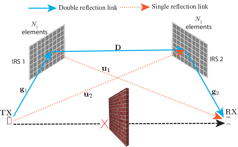
Based on a block-fading model with independent channel realizations across different coherence blocks, we denote ${\mathbf{g}}_{1}\in\mathbb{C}^{N_{1}\times 1}$, ${\mathbf{D}}\in\mathbb{C}^{N_{2}\times N_{1}}$, ${\mathbf{g}}_{2}\in\mathbb{C}^{N_{2}\times 1}$, ${\mathbf{u}}_{1}\in\mathbb{C}^{N_{1}\times 1}$, and ${\mathbf{u}}_{2}\in\mathbb{C}^{N_{2}\times 1}$ as the channel vectors from the Tx to IRS $1$, from IRS $1$ to IRS $2$, from IRS $2$ to the Rx, from IRS $1$ to the Rx, and from the Tx to IRS $2$, respectively. Taking into account for correlated Rayleigh fading and path-loss,¹¹ 1 The analysis could be easily extended to account for correlated Rician fading, where a LoS component exists additionally to a multipath part but this is the topic of future work. we have ${\mathbf{g}}_{1}\sim\mathcal{CN}\left({\mathbf{0}},{\mathbf{R}}_{t1}\right)$, $\mathrm{vec}({\mathbf{D}})\sim\mathcal{CN}\left({\mathbf{0}},{\mathbf{R}}_{12}\right)$, ${\mathbf{g}}_{2}\sim\mathcal{CN}\left({\mathbf{0}},{\mathbf{R}}_{2r}\right)$, ${\mathbf{u}}_{1}\sim\mathcal{CN}\left({\mathbf{0}},{\mathbf{R}}_{1r}\right)$, and ${\mathbf{u}}_{2}\sim\mathcal{CN}\left({\mathbf{0}},{\mathbf{R}}_{t2}\right)$, where ${\mathbf{R}}_{t1}=\beta_{t1}{\mathbf{R}}_{1}\in\mathbb{C}^{N_{1}\times N_{1}}$, ${\mathbf{R}}_{12}=\beta_{12}{\mathbf{R}}_{1}\otimes{\mathbf{R}}_{2}\in\mathbb{C}^{N_{1}N_{2}\times N_{1}N_{2}}$, ${\mathbf{R}}_{2r}=\beta_{2r}{\mathbf{R}}_{2}\in\mathbb{C}^{N_{2}\times N_{2}}$, ${\mathbf{R}}_{1r}=\beta_{1r}{\mathbf{R}}_{1}\in\mathbb{C}^{N_{1}\times N_{1}}$, and ${\mathbf{R}}_{t2}=\beta_{t2}{\mathbf{R}}_{2}\in\mathbb{C}^{N_{2}\times N_{2}}$ are the spatial covariance matrices of the respective links with $\beta_{t1}$, $\beta_{12}$, $\beta_{2r}$, $\beta_{1r}$, and $\beta_{t2}$ being the path-losses and ${\mathbf{R}}_{1}\in\mathbb{C}^{N_{1}\times N_{1}}$, ${\mathbf{R}}_{2}\in\mathbb{C}^{N_{2}\times N_{2}}$ being the correlation matrices of IRS $1$ and IRS $2$. Note that the path-losses and the covariance matrices are assumed known while they can be obtained with practical methods, e.g., see [16]. Similar to [7, 8], we assume receive RF chains integrated into the IRSs. These chains have sensing abilities and enable the acquisition of the CSI of individual channels. In particular, concerning the correlation model, we have considered a suitable model for IRSs, which is obtained under the conditions of rectangular IRSs and isotropic Rayleigh fading [15]. Specifically, let $d_{\mathrm{V}}$ and $d_{\mathrm{H}}$ denote the vertical height and horizontal width of each IRS element (both IRSs are constructed in the same way and have the same size of elements). Then, the $\left(i,j\right)$th element of the corresponding correlation matrix ${\mathbf{R}}\in\mathbb{C}^{N\times N}$ of the channels above in the case of an IRS with $N=N_{\mathrm{H}}N_{\mathrm{V}}$ elements is given by

where $\mathbf{u}_{\epsilon}=[0,\mod(\epsilon-1,N_{\mathrm{H}})d_{\mathrm{H}},\lfloor(\epsilon-1)/N_{\mathrm{H}}\rfloor d_{\mathrm{V}}]^{\scriptscriptstyle\mathsf{T}}$, $\epsilon\in\{i,j\}$, and $\lambda$ is the wavelength of the plane wave while $N_{\mathrm{H}}$ and $N_{\mathrm{V}}$ denote the elements per row and per column of the two-dimensional rectangular IRS.

Relying on a slowly varying flat-fading narrowband channel model, the complex-valued received signal at the Rx through the double IRS assisted network is expressed by

where ${\bm{\Phi}}_{i}=\mathrm{diag}\left(\alpha_{i1}\exp\left(j\theta_{i1}\right),\ldots,\alpha_{iN}\exp\left(j\theta_{iN_{i}}\right)\right)\in\mathbb{C}^{N_{i}\times N_{i}}$ expresses the reflecting beamforming matrix of the $i$th IRS, which depends on its elements with $\theta_{in}\in\left[0,2\pi\right]$ and $\alpha_{in}\in(0,1],n=1,\ldots,N_{i}$ being the phase shifts and the fixed amplitude reflection coefficients of the corresponding element of the $ith$ IRS ($i=1,2$). The progress on loss-less meta-surfaces allows to assume maximum reflection, i.e., we set $\alpha_{in}=1,\forall\penalty\ i,n$ [2].²² 2 Recently, it was shown that the amplitude and phase responses are intertwined in practice, while the assumption of unity amplitude is unrealistic [17]. However, the unity assumption amplitude still allows to reveal fundamental properties of the coverage probability of the proposed model. The consideration of the phase shift model in [17] suggests an interesting idea for extension of the current work, i.e., to study the impact of coverage probability of double-IRS assisted systems by accounting for this intertwinement. Moreover, $x$ expresses the transmitted data symbol satisfying $\mathbb{E}[|x|^{2}]\!=\!P$ with $P$ being the average power of the symbol, and $z\sim\mathcal{CN}\left(0,N_{0}\right)$ expresses the additive white Gaussian noise (AWGN) sample.

In this section, we present the derivation of the coverage probability when the double IRS assisted communication underlies to correlated Rayleigh fading by applying DE analysis tools [18].

We consider a three-dimensional Cartesian coordinate system, where the locations of the Tx, Rx, IRS $1$, and IRS $2$ together with the directions of the IRSs follow the lines in [6] to avoid repetition and for the sake of comparison. Similarly, the distances between the Tx and IRS $1$, between IRS $1$ and IRS $2$, and between IRS $2$ and Rx are $r_{t1}=1\penalty\ \mathrm{m}$, $r_{12}=100\penalty\ \mathrm{m}$, and $r_{2r}=15\penalty\ \mathrm{m}$. In this work, similar to [6, 7], we assume that the IRS in the single-IRS (baseline) case is located at a distance $\tilde{r}_{t}\approx r_{12}$ to result in nearly the same “product distance” for the two cases, i.e., $\tilde{r}_{t}\tilde{r}_{r}\approx r_{t1}r_{12}r_{2r}$, which means $\tilde{r}_{r}=r_{2r}$ since $r_{t1}=1\penalty\ \mathrm{m}$. Basically, this means that the IRS in the single-IRS case is located at the position of IRS $2$ in the double-IRS case. The size of each IRS element is given by $d_{\mathrm{H}}\!=\!d_{\mathrm{V}}\!=\!\lambda/8$ [15]. The spatial correlation matrix for each IRS is given by (1). Moreover, the path-loss exponents for the Tx-IRS $1$ and IRS $2$-Rx links are set as $2.2$, assuming that the IRSs are close to the corresponding Tx, Rx with no special obstacles in the intermediate space while the path-loss exponent for the IRS $1$-IRS $2$ link is set as $3$ since the second IRS is expected to be placed at a long distance, where the Rx will suffer from stronger signal attenuation. The path-loss exponents of the Tx-IRS $1$ and IRS $2$-Rx links are set to this value since we have assumed that these links approach LoS conditions due to the smart placement of the IRSs near the Tx and Rx toward better communication. A similar exponent is assumed for the single reflection links, i.e., $2.2$ and $3$ for the first and second link, respectively. The carrier frequency is $3$ GHz, the system bandwidth is $10$ MHz, $P=43\penalty\ \mathrm{dBm}$, and the noise variance is $-94$ dBm.

Fig. 2.a illustrates the coverage probability versus the target rate for varying $N_{1}$ based on Proposition 2. Specifically, given a specific number of total elements $N=200$, we vary $N_{1}$. We observe that by increasing the number of elements in IRS $1$, $P_{\mathrm{c}}$ increases until $N_{1}=100$ elements and then starts decreasing. In other words, we notice the highest coverage when the two IRS are implemented with almost the same number of elements, which agrees with [6, 7]. Moreover, MC simulations almost coincide with the analytical results, which corroborates that Alzer’s inequality, the selected value of $M$, and the DE analysis are valid approximations. In the same figure, we show the coverage probability of the single-IRS SISO channel for $N=100$ and $N=200$ elements under the same conditions and we observe that the double-IRS cooperative system presents better performance.

In Fig. 2.b, we depict the coverage probability versus the target rate for different settings. First, we focus on the impact of correlation. In particular, in the case of no correlation, $P_{\mathrm{c}}$ is lower since the covariance matrix of the overall channel, found in the DE SNR, does not depend on the RBMs, and thus, cannot be optimized. This observation coincides with the results in [13] for single-IRS-assisted communication. In the case of correlation, if the correlation increases, e.g., due to decrease of the inter-element distance, $P_{\mathrm{c}}$ decreases. Moreover, if random phases shifts are assumed in both IRSs, the coverage is much lower, which means that the RBM optimization definitely improves the performance. Also, we depict the performance of the single-IRS-assisted scenario for the above considerations and we observe that the double-IRS architecture provides better coverage as expected.

In 2.c, we demonstrate the convergence of the proposed algorithm, i.e., $(\mathcal{P}1)$ in (8). Specifically, we have depicted the coverage probability versus the number of iterations for various numbers of IRS elements. As can be seen, the algorithm converges fast in all cases. For example, when $N_{1}=50$ , the algorithm converges in $9$ iterations. In addition, we observe that by increasing the IRS in terms of its elements, more iterations are required for convergence because the amount of optimization variables increases and the corresponding search space is enlarged. Also, an increase in terms of IRS elements results in higher complexity of each iteration of the algorithm as mentioned in Sec. III.B.

In this paper, we derived the coverage probability of a double-IRS-assisted SISO system under the realistic conditions of correlated Rayleigh fading. Specifically, for given RBMs, we obtained its novel expression in closed-form in terms of only large-scale statistics. Moreover, the proposed optimization over the RBMs exhibits a great advantage concerning the reduction of the computational complexity since it can be performed not at each coherence interval but once per several intervals. Among others, numerical results showed the outperformance of double-IRS systems over single-IRS systems and the impact of correlated Rayleigh fading. Future works on the coverage of double-IRS assisted systems could elaborate on the design of multi-user and multi-antenna transmission, and possibly, the impact of Rician fading.

References

- [1] Q. Wu and R. Zhang, “Towards smart and reconfigurable environment: Intelligent reflecting surface aided wireless network,” IEEE Commun. Mag., vol. 58, no. 1, pp. 106–112, 2020.
- [2] E. Björnson, Ö. Özdogan, and E. G. Larsson, “Intelligent reflecting surface versus decode-and-forward: How large surfaces are needed to beat relaying?” IEEE Wireless Commun. Lett., vol. 9, no. 2, pp. 244–248, 2019.
- [3] A. Kammoun et al., “Asymptotic max-min sinr analysis of reconfigurable intelligent surface assisted MISO systems,” IEEE Trans. Wireless Commun., vol. 19, no. 12, pp. 7748–7764, 2020.
- [4] A. M. Elbir et al., “Deep channel learning for large intelligent surfaces aided mm-Wave massive MIMO systems,” IEEE Wireless Commun. Lett., vol. 9, no. 9, pp. 1447–1451, 2020.
- [5] A. Papazafeiropoulos et al., “Intelligent reflecting surface-assisted MU-MISO systems with imperfect hardware: Channel estimation and beamforming design,” IEEE Trans. Wireless Commun., pp. 1–1, 2021.
- [6] Y. Han et al., “Cooperative double-IRS aided communication: Beamforming design and power scaling,” IEEE Wireless Commun. Lett., vol. 9, no. 8, pp. 1206–1210, 2020.
- [7] B. Zheng, C. You, and R. Zhang, “Double-IRS assisted multi-user MIMO: Cooperative passive beamforming design,” IEEE Trans. Wireless Commun., pp. 1–1, 2021.
- [8] B. Zheng, C. You, and R. Zhang, “Efficient channel estimation for double-IRS aided multi-user MIMO system,” IEEE Trans. Commun., vol. 69, no. 6, pp. 3818–3832, 2021.
- [9] Q. Wu and R. Zhang, “Intelligent reflecting surface enhanced wireless network via joint active and passive beamforming,” IEEE Trans. Wireless Commun., vol. 18, no. 11, pp. 5394–5409, 2019.
- [10] C. Guo et al., “Outage probability analysis and minimization in intelligent reflecting surface-assisted MISO systems,” IEEE Commun. Lett., vol. 24, no. 7, pp. 1563–1567, 2020.
- [11] L. Yang et al., “Coverage, probability of SNR gain, and DOR analysis of RIS-aided communication systems,” IEEE Wireless Commun. Lett., vol. 9, no. 8, pp. 1268–1272, 2020.
- [12] T. Van Chien et al., “Outage probability analysis of IRS-assisted systems under spatially correlated channels,” IEEE Wireless Commun. Lett., vol. 10, no. 8, pp. 1815–1819, 2021.
- [13] A. Papazafeiropoulos et al., “Coverage probability of distributed IRS systems under spatially correlated channels,” IEEE Wireless Commun Lett., vol. 10, no. 8, pp. 1722–1726, 2021.
- [14] A. Papazafeiropoulos et al., “Asymptotic analysis of Max-Min weighted SINR for IRS-assisted MISO systems with hardware impairments,” IEEE Wireless Commun. Lett., pp. 1–1, 2021.
- [15] E. Björnson and L. Sanguinetti, “Rayleigh fading modeling and channel hardening for reconfigurable intelligent surfaces,” IEEE Wireless Commun. Lett., vol. 10, no. 4, pp. 830–834, 2021.
- [16] D. Neumann, M. Joham, and W. Utschick, “Covariance matrix estimation in massive MIMO,” IEEE Signal Process. Lett., vol. 25, no. 6, pp. 863–867, 2018.
- [17] S. Abeywickrama et al., “Intelligent reflecting surface: Practical phase shift model and beamforming optimization,” IEEE Trans. Commun., vol. 68, no. 9, pp. 5849–5863.
- [18] A. K. Papazafeiropoulos and T. Ratnarajah, “Deterministic equivalent performance analysis of time-varying massive MIMO systems,” IEEE Trans. Wireless Commun., vol. 14, no. 10, pp. 5795–5809, 2015.
- [19] S. Boyd, S. P. Boyd, and L. Vandenberghe, Convex optimization. Cambridge university press, 2004.
- [20] H. Alzer, “On some inequalities for the incomplete gamma function,” Mathematics of Computation of the American Mathematical Society, vol. 66, no. 218, pp. 771–778, 1997.
- [21] T. Bai and R. W. Heath, “Coverage and rate analysis for millimeter-wave cellular networks,” IEEE Trans. on Wireless Commun., vol. 14, no. 2, pp. 1100–1114, 2015.