Kink-antikink scattering in a quantum vacuum
Abstract
We study kink-antikink scattering in the sine-Gordon model in the presence of interactions with an additional scalar field, , that is in its quantum vacuum. In contrast to the classical scattering, now there is quantum radiation of quanta and the kink-antikink may form bound states that resemble breathers of the sine-Gordon model. We quantify the rate of radiation and map the parameters for which bound states are formed. Even these bound states radiate and decay, and eventually there is a transition into long-lived oscillons.
1 Introduction
Topological defects are expected to arise during phase transitions in the early universe. These can include domain walls Saikawa:2020duz; Hiramatsu:2012sc; Vilenkin:1982ks; Sikivie:1982qv, cosmic strings Vilenkin:1984ib; Blanco-Pillado:2017rnf; Dufaux:2010cf; Damour:2000wa; Albrecht:1984xv; Vachaspati:1984gt; Hindmarsh:1994re; Kibble:1976sj, monopoles tHooft:1974kcl; Nambu:1974zg; Gibbons:1986df; Mavromatos:2020gwk and textures Gueron:1997ck; Notzold:1990jt; Spergel:1992ff; Durrer:1990qe; Turok:1989ai; Brandenberger:2019txi, depending on the symmetry breaking pattern. While topological defects have not yet been observed in a cosmological context Planck:2013mgr, they are abundant in condensed matter systems Zurek:1985qw; PhysRevLett.119.013902; PhysRevLett.105.075701; Chuang:1991zz; Bowick:1992rz; Hendry1994; Ruutu1996; Bauerle1996; PhysRevLett.89.080603; PhysRevLett.84.4966; PhysRevLett.91.197001; Beugnon2017, with intriguing analogies between the two areas of research Kibble:2001wj; Vachaspati:1998vc; Zurek:1996sj.
Topological defects are also an ideal setting for studying quantum effects in spacetime dependent classical backgrounds. Significant effort has already gone into the quantization of topological defects Rajaraman:1982is; Coleman:1985rnk; Christ:1975wt; Goldstone:1974gf; Cahill:1974cs; Dashen:1974ci; Dashen:1974cj; Dashen:1974ck, in which case the topological defects form space-dependent backgrounds for quantum fields. Less effort has been invested in time-dependent problems that involve quantum fields in the background of dynamical topological defects Dashen:1975hd. Going one step further, the quantum fields will backreact on the dynamics of the topological defects and lead to non-trivial interplay between the quantum and classical degrees of freedom. This is the subject of the present paper.
The sine-Gordon equation in one spatial dimension holds a special place in the soliton literature, since it is integrable and allows for the construction of multi-soliton solutions by the use of the Bäcklund transformation. The solitons (or kinks) of the sine-Gordon equation are solutions which interpolate between two successive minima of the potential. The sine-Gordon model has been analyzed in great detail Rajaraman:1982is; Coleman:1985rnk; Vachaspati:2006zz and kink-antikink scattering is known to be trivial – the kink and antikink pass through each other albeit with a time delay – a result that holds even when is treated in quantum field theory. scattering in a model where the sine-Gordon scalar field, , is coupled to a second scalar field, . The kink and antikink propagate in the quantum vacuum of , deforming the vacuum around them. (Alternately, the kink and antikink get dressed by the field.) Upon kink-antikink scattering, particles (wavepackets) are radiated. Depending on the parameters, the quantum radiation of particles can lead to the production of a kink-antikink bound state that is known as a “breather” in the sine-Gordon literature Rajaraman:1982is; Coleman:1985rnk; Vachaspati:2006zz. In this case, the breather oscillates and continues to radiate particles. (This was more specifically studied in Ref. Olle:2019skb, albeit in a slightly different model.) Surprisingly we find that the breather eventually settles into another oscillating configuration that radiates very slowly, resembling an “oscillon”. Oscillons are long-lived localized configurations arising in a variety of scalar field theories and have been shown to emerge naturally in scenarios ranging from preheating to bubble collisions (see e.g. Amin:2011hj; Copeland:1995fq; Gleiser:2009ys; Farhi:2005rz; Graham:2006vy; Zhou:2013tsa; Fodor:2008es; Hiramatsu:2020obh; VanDissel:2020umg; Zhang:2020bec; Zhang:2020ntm).
Our analysis is enabled by the “classical-quantum correspondence” (CQC) in which the dynamics of free quantum fields in spacetime dependent classical backgrounds has been shown to be equivalent to a completely classical problem in higher dimensions Vachaspati:2018hcu; Olle:2019skb; Mukhopadhyay:2019hnb. Quantum backreaction on the classical background is included in the analysis in the semiclassical approximation in which quantum operators occurring in the classical equations of motion are replaced by their dynamical expectation values. Special attention is given to the renormalization issues that arise, since a divergent part of the expectation values contributes to the mass parameter of the background field.
In Sec. 2 we introduce the field theoretic model, as well as the equations that will be solved numerically to determine the full dynamics of the kink-antikink collision. We take care to distinguish the no backreaction case, where the kink-antikink background is fixed, from the general case with backreaction. In Secs. 3 and 4 we outline the results of our numerical analysis: we determine the region of parameter space where a breather-like bound state is formed after the collision and discuss the different phases of its decay. We conclude in Sec. 5, where we discuss the implications of this work, its limitations as well as several future prospects. We use natural units where throughout.
2 Setup
We work in 1+1 dimensions and consider a sine-Gordon field coupled to a massive scalar field according to the Lagrangian density
| (1) |
Here , are the masses of the two fields, is a parameter introduced for future convenience and is a coupling constant. We will assume that conditions are such that the field can be treated classically, while the field is treated fully quantum mechanically. In general, the (potentially space and time-dependent) classical “background” field excites the quantum “radiation” field , and the excitations of in turn backreact on . In the following it will be useful to make the field redefinition and to work with the rescaled field . With this new field variable, the Lagrangian density becomes
| (2) |
We see that the coupling between the two fields and is such that the discrete shift symmetry , , is maintained.
2.1 Neglecting backreaction
2.1.1 Background dynamics
We start by discussing the limit which corresponds to the case where the dynamics of the field doesn’t feel the presence of the radiation field . If is entirely neglected, this is also the limit when is classical because, in the path integral, is equivalent to . In this “no backreaction” case, the field equation reduces to the sine-Gordon equation
| (3) |
It is worth mentioning that, in this case, one can define the (conserved) energy of the sine-Gordon field unambiguously by
| (4) |
and it is easy to see that the limit is equivalent to the energy of the sine-Gordon field being much larger than the (renormalized) vacuum energy of the field . We will come back to this point in Sec. 4.
Eq. (3) has well-known kink and anti-kink solutions,
| (5) |
which describe a soliton (or antisoliton depending on the sign) whose center is at at time and which moves to the right with velocity , with being the Lorentz factor. It is worth noting that the energy of this configuration is
| (6) |
The integrability properties of the sine-Gordon equation allow for the analytical construction of more complicated solutions involving a kink and an antikink. The first one is the so-called breather solution which can be understood as a bound state of a kink and an antikink and which reads
| (7) |
Here is the angular frequency of the breather and . The energy of the breather is
| (8) |
and is seen to be less than the sum of the energy of a static kink and a static antikink.
The other important solution, which will be the main focus of our attention in the remainder of this paper, can be obtained from the breather solution by making the formal substitution . It reads
| (9) |
and describes the elastic scattering of a kink and an antikink infinitely separated at and moving towards each other with velocity . The collision occurs at and the kink and antikink pass through each other with a time delay. As expected, the energy of this field configuration is simply the sum of the energies of a kink and an antikink moving with velocity ,
| (10) |
Having summarized some important features of the sine-Gordon equation, we are ready to study the quantum field living in the background of the latter solution.
2.1.2 Quantum radiation
Integrability of the sine-Gordon model implies that the scattering of a kink-antikink pair is trivial i.e. never forms a bound state, and that a breather never decays. These are classical properties of the sine-Gordon model but they are maintained when taking the quantum fluctuations of the field into account. However, in our case, the classical sine-Gordon field is coupled to an external quantum scalar field and the energy exchange between the classical field configuration and the quantum bath is expected to invalidate these properties.
We thus turn our attention to the quantum radiation that occurs during kink-antikink scattering, equivalently particle production in the time-dependent background given in Eq. (9), using the framework of the classical- quantum correspondence (CQC) Vachaspati:2018llo; Vachaspati:2018hcu; Olle:2019skb that we briefly describe below. Since in the limit the dynamics of the background field is insensitive to the presence of the field , we will work with the truncated Lagrangian density
| (11) |
It is easy to understand why this model leads to excitations of the quantum field . Indeed this Lagrangian density describes a free scalar field with a space and time dependent mass-squared . The non-adiabatic variation of will lead to particle production and is expected to occur mostly at the time of kink-antikink collision at .
To study the scattering more quantitatively using numerical methods, we start by compactifying the spatial dimension on a circle of length which we then discretize on a regular lattice consisting of evenly spaced points. The lattice spacing is therefore . We can further define the discretized field values and for , and use the following differencing scheme to estimate the second spatial derivative,
| (12) |
With these conventions, and after a spatial integration by parts, the Lagrangian of this discretized model can be written as
| (13) |
where we have arranged the discretized values of the field in a column vector and introduced the matrix
| (14) |
In this form, the discretized Lagrangian is immediately seen to describe a collection of harmonic oscillators (located at each lattice point) coupled to each other via quadratic interactions. The total energy and energy density at each lattice point for the field in this discretized model are also well-defined and given by11 1 Here, in order to get a more accurate discretized estimate of the local gradient energy, the average between its forward differencing and backward differencing approximations is used. This allows us to integrate Eq. (16) into Eq. (15). Notice however that simply choosing a forward or backward differencing scheme for the estimation of this component of the energy density would also have been consistent.
| (15) | |||||
| (16) |
The next step is to quantize the theory (in the Heisenberg picture) by promoting the discretized field values to operators and introducing the time-dependent matrix whose (complex) elements satisfy the relation
| (17) |
Here the reference time is chosen so that the background for can be approximated by a slowly-moving kink-antikink pair separated by a large distance (much larger than their typical size). This is equivalent to specifying a reference vacuum state , the state annihilated by all the . (The ladder operators and refer to the quantum harmonic oscillators located at each lattice point.) Now the dynamics of the field is simply given by the Heisenberg equations
| (18) |
with initial conditions
| (19) |
Since is a symmetric positive definite matrix, is computed by first diagonalizing and then applying the desired power function to its positive eigenvalues. Notice that these initial conditions only define the vacuum of the theory unambiguously when the background is approximately constant for . In other words if the time evolution of the background before the time is adiabatically slow, a different choice of initial time smaller than will not modify the quantum dynamics. More precisely the initial conditions (19) define the -th order adiabatic vacuum (which corresponds to the lowest order approximation of the mode functions within the WKB approximation Birrell:1982ix). In particular, if the background is such that no obeying the required properties can be found, then we can expect spurious excitations of the field to occur and one should strive to minimize them. In the case at hand, the kink and antikink are moving towards each other with velocity at and we find ourselves exactly in the latter situation. However, we expect that for small (in practice less than ) the initial conditions (19) will still give reasonable results (and we will come back to this later in Sec. 3).
2.1.3 Observables
The evolution of is given by the system of equations given in matrix form in Eq. (18). Initialized by Eqs. (19), they are particularly simple and they can readily be solved numerically. Moreover, the variables allow for the easy computation of various observable quantities of interest. For example, the expression for the vacuum expectation value of the energy in the radiation field can be written as
| (20) |
This is equal to the total (classical) energy in the variables. Similarly, the vacuum expectation value of the energy density at the -th lattice point is
| (21) |
Moreover the spatial two-point function of the radiation field can be written as
| (22) |
In order to render these expressions insensitive to the discretization scale , we first renormalize the spatial two-point function by subtracting its counterpart,
| (23) |
and then use it to renormalize the -dependent part of the energy and energy density. This procedure is closely related to point-splitting Birrell:1982ix. The resulting renormalized quantities are thus
| (24) | |||||
| (25) |
In both these equations, the last term corresponds to the subtraction of the (constant) zero-point energy.
We can therefore compute any quantity of interest for the study of particle production in the background by studying the classical dynamics of the variables (with well-chosen initial conditions). We thus trade real quantum variables (corresponding to the discretized field values ) for complex classical variables (the ). This is the essence of the CQC and it is closely related to the mode function and Bogoliubov coeffcient methods Vachaspati:2018hcu.
2.1.4 Initial conditions and vacuum structure
The renormalized energy density observable allows us to visualize the vacuum structure of the quantum field . Fig. 1 shows the renormalized energy density in the field at the initial time superimposed over the background kink-antikink profile. (The parameter will always be chosen such that the lattice provides a good approximation of the continuum limit and therefore we will liberally identify the discretized quantities and to their continuous counterparts and for .) We see that the presence of the background induces a dip in the energy density around the kink and antikink, akin to two clouds of particles. The width of these clouds is set by the kink and antikink width i.e. . However, as shown in Fig. 2, the depth of the underdensities depends on the coupling and the mass of the field . In particular, the trough of the energy density around the kink-antikink position increases for larger and smaller . Moreover, for some parameters, the energy density of shows some non-trivial features that reflect the relevance of the additional length scales and .
2.2 Including backreaction
The results above assumed that backreaction can be neglected. This is certainly a good approximation when is small but what happens when backreaction can no longer be neglected? This constitutes the main part of this work, to which we now turn.
We thus consider the case so that the field equation for the field gets a contribution from the field:
| (26) |
Of course this equation is fully classical and one would need to decide how the quantum excitations in the field couple to the classical background by modifying the coupling term proportional to . The most straightforward way is to use the semiclassical approximation22 2 Another procedure for incorporating backreaction is based on the stochastic method, where the initial conditions for the field are sampled from a distribution similar to Eq. (19). Several simulations, each with different samples for the initial conditions, would be performed and then averaged. We leave the interesting comparison between the two methods for future work. which simply entails replacing by . Therefore the field equation becomes
| (27) |
To make contact with the methods described in the previous section, we need the discretized version of this equation,
| (28) |
where is not given by the non-dynamical kink-antikink solution anymore, rather it will have to be solved for subject to the initial conditions and . Solving Eq. (28) requires being able to compute the dynamics of the quantity . This can be done by using the results of the previous section and in particular Eq. (22) to make the substitution
| (29) |
with given by Eqs. (18) and (19), where background field values in the definition of are replaced by the corresponding dynamical values. Because is a 1+1 dimensional two-point function in the coincident point limit, in other words given in Eq. (22), it is logarithmically sensitive to the discretization scale , and it would produce infinite backreaction in the continuum limit Vachaspati:2018llo; Vachaspati:2018hcu; Olle:2019skb. This can be remedied by noticing that the parameter appearing in the field equations is actually the bare mass of the sine-Gordon field, and using it to renormalize the divergence. We therefore define the physical mass of the sine-Gordon field by
| (30) |
Here, in the second equality, we used the fact that, when , is a constant matrix, and therefore Eq. (18) has the simple solution
| (31) |
Moreover in the third equality of Eq. (30) we use the fact that all the diagonal coefficients of the matrix are equal to each other (see Eq. (14)). Overall this procedure is equivalent to replacing the two-point function by its renormalized counterpart in Eq. (28), and by in every equation where it appears. Notice that, in the non-backreacting case (), the bare mass and the physical mass are one and the same. Henceforth, we will simply choose when taking backreaction into account.
Summing up, the backreacted dynamics (within the semiclassical approximation) are given by the system of coupled differential equations
| (32) |
and
| (33) |
with initial conditions
| (34) | |||||
| (35) |
where we recall that
| (36) |
and where the matrix defined in Eq. (14) depends on the fully dynamical background . Note that the mass of the field used in the initial conditions is the physical mass , as shown in the above equation.
Before discussing the results of our simulations, let us say a few words about the observables that we are going to use in our study of particle production and the associated backreaction during kink-antikink collisions. These need to accurately account for the energy exchanged between the background and the quantum radiation bath. Of course, in general, in a fully interacting theory it is impossible to separate the energy of a particular subsystem. However, as long as the coupling is not too big (smaller than in practice) we can assume that Eqs. (25) and (24) still provide a useful measure of the (renormalized) energy, respectively energy density, in the quantum field . Under these assumptions, the energy in the kink-antikink background is given by
| (37) |
Notice that the total (conserved) energy of the coupled system is given by
| (38) |
3 Results
In this section we present our numerical results. We will always work in units where . which is equivalent to rescaling space, time, and by . Our lattice is a circle of physical size and is sampled by equally spaced points (). We use an explicit Crank-Nicholson method with two iterations to solve the system of coupled ordinary differential equations given in Eqs. (32) and (33) with the initial conditions of Eqs. (34) and (35). The initial time is taken to be . Because most interesting effects are expected to occur at or around the time of collision, , and to make sure that finite lattice size effects don’t spoil any physical effects, we only evolve the equations for one light-crossing time after the collision i.e. up to . We have also made sure that the results do not strongly depend on the UV and IR cutoffs ( and ) and that our renormalization scheme is sufficient to eliminate any UV sensitivity (see Fig. 16). Of course, decreasing would improve the resolution of the simulations but, given the complexity of the code, this is not feasible without significantly more computational cost. Similarly a larger lattice would allow us to track the dynamics of the system for a longer time but maintaining spatial resolution would again require a corresponding increase in . In the current work, energy non-conservation due to numerical error over the whole duration of time evolution is of the order of .
The range over which we will vary the different parameters , and will depend on numerical accuracy as well as on the intrinsic limitations of our model. To avoid strong coupling effects we will be allowing to vary between 0 and 1. Since our initial conditions for the variables are strictly only valid when the background is adiabatically varying, we limit ourselves to velocities smaller than 0.3.33 3 Because of this violation of adiabaticity at , a small amount of spurious particle production is observed for the case but the corresponding dissipated energy is of the order of of which can safely be neglected. Moreover, we require the kink-antikink pair to be well-separated at the initial time which, because of the finite size of our periodic lattice, limits the range of to the interval . Since the background field is assumed to behave classically, its mass is expected to be larger than the mass of the radiation field . Thus is constrained to be smaller than 1.
We start by presenting the two qualitatively different possible outcomes of the inelastic kink-antikink scattering studied in this paper: pure scattering, or formation of a bound state, i.e. a breather-like structure. Then we will discuss what role the different parameters of the model play in the occurrence of these two outcomes.
3.1 Scattering or formation of a bound state
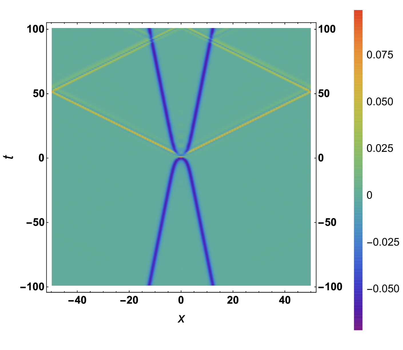
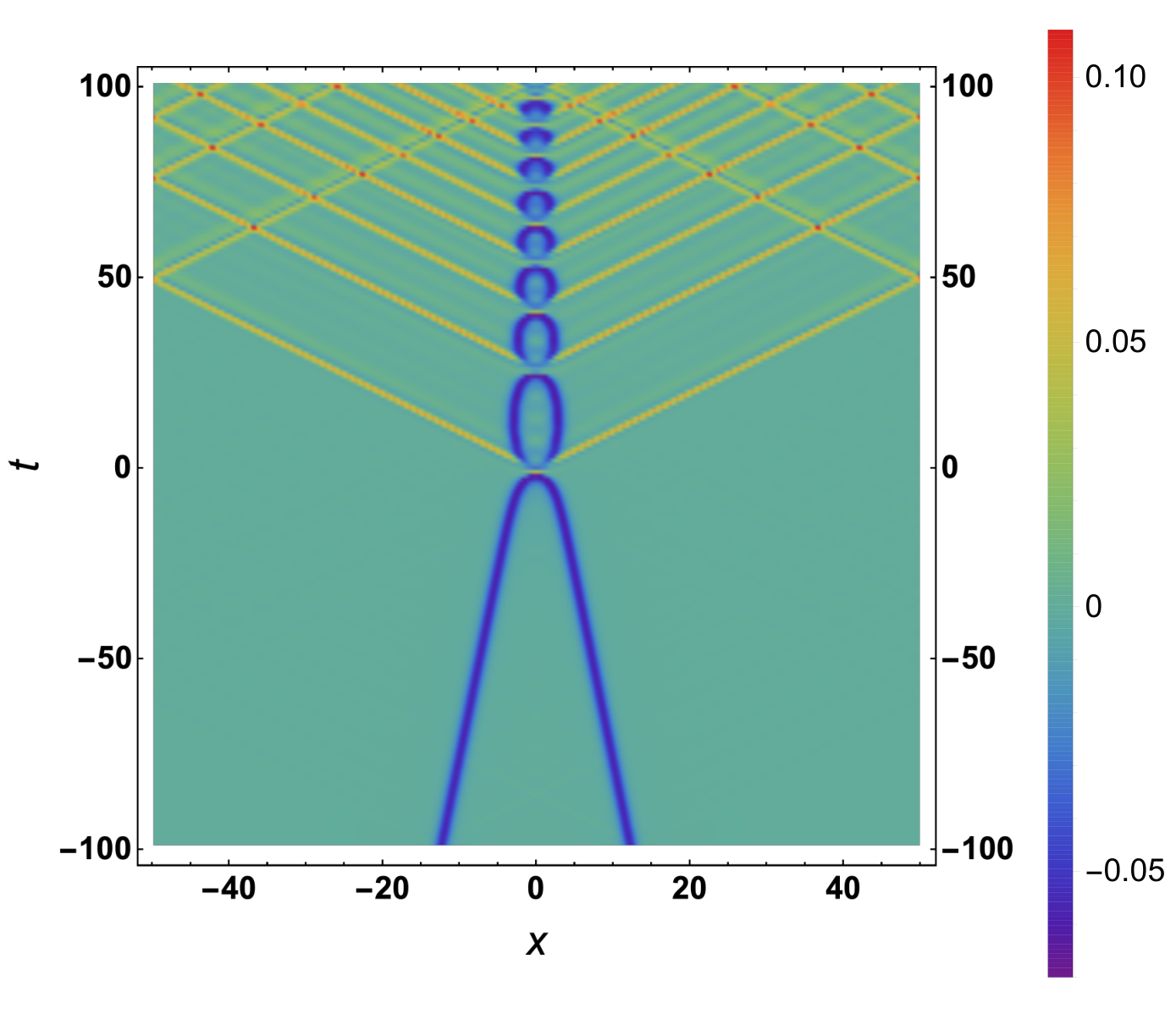
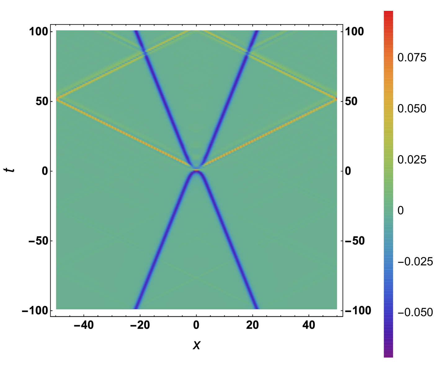
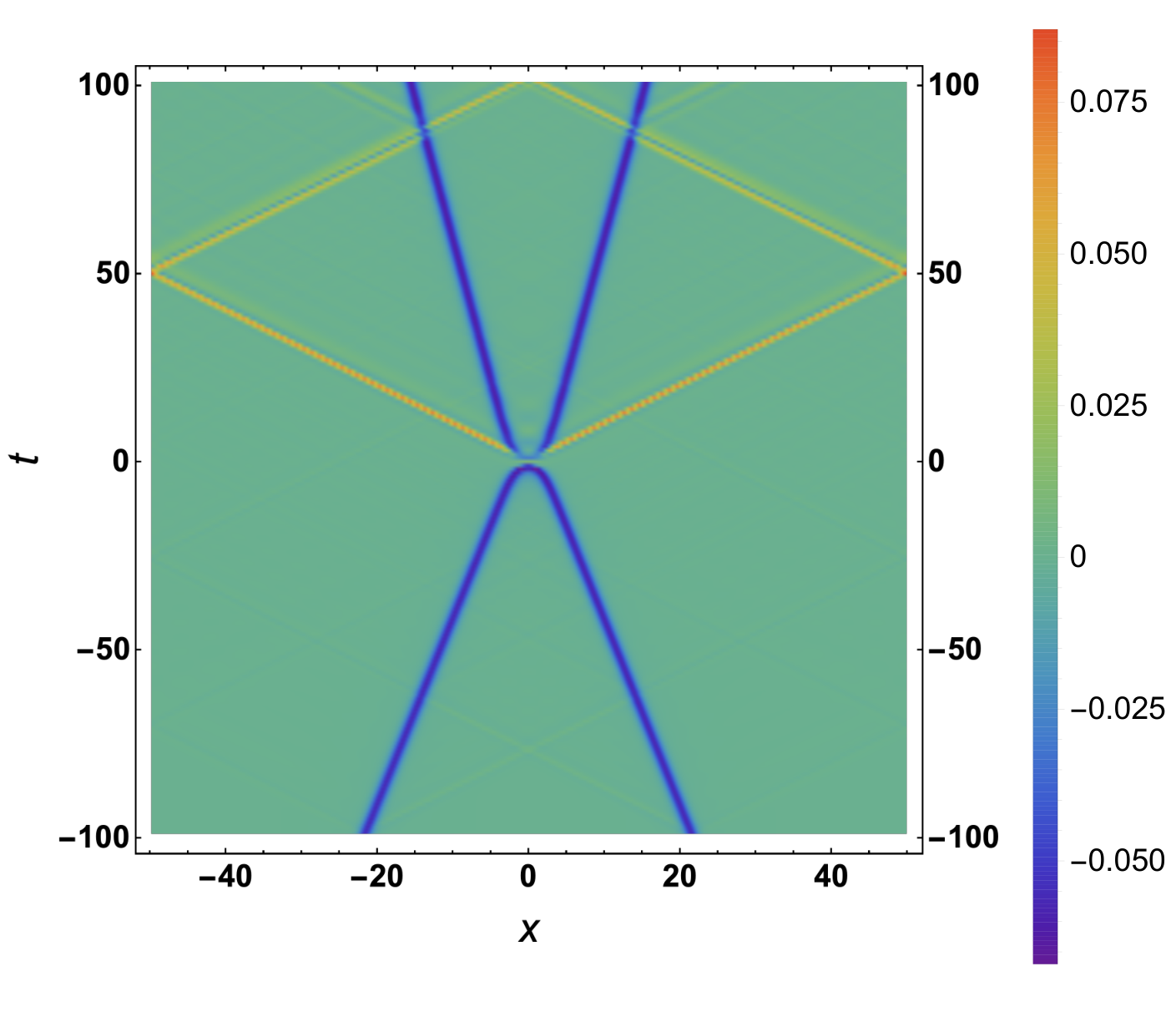
In Fig. 3 we show the renormalized energy density in the field as a function of (horizontal axis) and (vertical axis) with and without backreaction for two different sets of parameters. The color coding represents the value of the energy density from its minimum value in dark blue to its maximum value in bright red. Since the clouds of particles (thick dark blue lines) track the kink and antikink perfectly, this representation is particularly well suited for visualizing both the dynamics of the kink-antikink background and any radiation bursts (thin orange lines) occurring during their collision. It serves as an accurate spacetime diagram of the collision. The first thing we notice, in Figs. 3a and 3c, is that when i.e. when backreaction is neglected, the kink and antikink dynamics are unperturbed by the collision (as they should be); there are however two bursts of radiation originating and i.e. at the collision, and propagating away from the kink-antikink pair (one to the left the other to the right) at or near the speed of light. When reaching the end of the lattice they wrap around and come back towards the center by virtue of the periodic boundary conditions. The origin of the bursts of radiation can be explained intuitively by the high degree of non-adiabaticity of the background at the moment of collision.
More interestingly, Figs. 3b and 3d, including backreaction effects, show two radically distinct behaviors. In Fig. 3d, the parameters are such that the collision does not lead to the formation of a bound state. Just like in the non-backreacting case of Fig. 3c, the clouds of particles tracking the kink-antikink pair describe an X-like pattern: they are seen to converge, collide and subsequently diverge from one another. The collision is again accompanied by the emission of two bursts of radiation. However, unlike in Fig. 3c, the outgoing relative velocity of the kink-antikink pair in Fig. 3d is smaller than the initial velocity as background kinetic energy has been converted in quantum radiative energy. In Fig. 3b, the parameters are such that the collision leads to the formation of a breather-like kink-antikink bound state. The cactus (or caterpillar) pattern described by the clouds of particles after the initial collision at represents the multiple subsequent collisions that the kink and antikink undergo, each accompanied by a burst of radiative energy. The first burst of energy depletes enough kinetic energy that the kink and antikink are not able to break away from their mutual attraction and must form a bound state. We will study the evolution of the energy in , , in more detail in the next subsection.
3.2 Parameter dependence of the outcome of the collision
To understand the influence of the parameters of the model on the dynamics of the collision (with backreaction taken into account), we turn our attention to the energy in the kink-antikink pair. In Figs. 4, 5 and 6 we plot as a function of time for different values of the parameters , and . We can make a few general comments before going into the details of the plots. First we notice that before the collision is constant, which is to be expected because the kink and antikink are effectively decoupled until their relative distance becomes of the order of the kink width . At the collision, the energy decreases abruptly which corresponds to the initial burst of radiation seen in the previous subsection. The energy then quickly stabilizes to a new plateau. If the value of this new energy plateau is larger than the energy of a static kink-antikink pair i.e. , then a breather-like object does not form and the kink-antikink pair remains unbound after the collision ( remains constant after the collision). On the contrary, if the first burst of energy is large enough to make the value of the energy plateau fall below this threshold energy, then a bound state is formed. This is followed by a cascade of subsequent bursts of energy that lead to the decay of into lower and lower plateaus of shorter and shorter duration. This cascade is readily understood. After the first collision, the kinks separate out more than their widths which leads to the formation of an energy plateau (because kinks radiate only when they overlap). Eventually though, after a certain number of subsequent collisions, they don’t manage to separate out and the plateau shape is lost. The radiation thus transitions through different behaviors which we will discuss in more detail in the next section.
Figure 4 shows for , , and varying . The higher the initial relative velocity the bigger the gap to the threshold energy of bound state formation, , as seen from Eq. (10). We notice that the energy of the first radiation burst doesn’t depend strongly on (see Appendix A) and therefore, as long as it is larger than , a breather-like object is formed. This happens in particular for and .
Figure 5 shows for , , and varying . Here, the energy of the first radiation burst increases with (it approximately scales as for the range of parameters considered here) and exceeds for and , when a breather-like object forms. In the and cases we notice a peculiar change of behavior in around when the cascading decay becomes an oscillatory decay with a smaller average slope. The bound state then appears to settle to a long-lived, weakly radiating, oscillon-like object. We will come back to this intriguing configuration in the next section.
Figure 6 represents for , , and varying . Here we notice that the lighter the field, the stronger the initial radiation burst after collision (it scales as ). This is readily understood, as a light field is more easily excited by the time-dependent background. For , a breather-like object forms since the kink-antikink pair releases an energy greater than at the collision.
We can even go further and determine the region of parameter space where a breather-like object forms, i.e. the region where the first burst of energy at the collision is larger than . We expect that the boundary between the region where a bound state forms and the one where the kink-antikink pair remains unbound after collision, to approximately look like a two-dimensional surface. However, since our determination of is imperfect, particularly because the first energy plateau after collision exhibits small oscillations (as can be seen for instance in Figs. 4, 5 and 6), the boundary will necessarily have a thickness. To estimate this thickness we determine the characteristic amplitude of the small oscillations around the first energy plateau in the worst case scenario (by computing the standard deviation from the mean value in this case) and we conservatively declare that a first energy burst equal to with a margin of error of doesn’t allow us to definitively determine whether a bound state forms or not. Here . In Fig. 7 we show the results of a parameter scan with resolution of in , in and in .
4 Decay of the bound state
We have already seen that, when the parameters of the problem are such that a bound-state forms as a consequence of the kink-antikink collision, the radiation goes through different phases. In this section we highlight two of those phases: the fast decay phase where radiation is emitted via successive energy bursts, and the oscillon phase which is weakly radiating and quasi-stable.
4.1 The energy plateau phase: decay of the breather-like object
In cases where the kink and antikink scatter to form a bound state, we observed that there is a cascade of bursts of radiation at decreasing time intervals. In this subsection we focus on the blue curve in Fig. 4 corresponding to the choice of parameters , and . This case features particularly well-defined energy plateaus and lends itself to further analysis. We plot , the energy after the burst as a function of in Fig. 9a and find the fit
| (39) |
where is the initial energy. Using Fig. 8 we can also characterize the time intervals between the and bursts (or between two successive zeros of ), as shown in Fig. 9b, to get the fit
| (40) |
where is the first burst interval. We can then eliminate to obtain the relation between and ,
| (41) |
Using the exact solution for the sine-Gordon breathers, the relation between the energy and the half-period is
| (42) |
Fig. 10 shows an excellent agreement of the numerical data with the analytic sine-Gordon prediction for the relation between the plateau energy and the half-period, showing that the field decay proceeds discretely through a series of breather states. This decay of the energy continues for a finite number of bursts and then, at a critical time, the system rapidly decays into a new, more stable, oscillon-like phase (which we study in more detail in the next subsection).
4.2 Formation of a long-lived oscillon


In this subsection we focus on the particular case , and (depicted in the blue curve of Fig. 5) which prominently features a long-lived oscillon phase and allows us to study its formation and decay. In Figs. 11a and 11b we show the time evolution of the energy densities in and respectively. In both cases, we see a qualitative change in the appearance of the breather-like structure occurring around : the spatial extension of the object ceases to decrease and its energy density undergoes small oscillations in amplitude (visible on both plots). Fig. 13 shows that the oscillations in the energy of are accompanied with out-of-phase oscillations in the localized energy of around the origin. As can be seen in Fig. 11b the onset of this new regime is preceded by a large burst of radiation that almost completely turns off at . Fig. 11c shows the amplitude of the value of the field at the center of the lattice as a function of time. This is in fact a good measure of the field profile amplitude. The same qualitative change of behavior is observed on this plot: starting with the moment of collision, the field profile undergoes oscillations of decaying amplitude until a new quasi-stable oscillatory regime is reached around . Although, the amplitude of oscillation continues to decrease, it does so at a very slow rate which justifies the long-lived oscillon nomenclature. Finally, Fig. 11d is simply a zoomed in version of the blue curve in Fig. 5 allowing us to fit a power law to the envelope of within the long-lived oscillon regime. We find a power law decay. This is to be contrasted to the approximately linear decay occurring during the immediately preceding phase, where, on average, the energy decreases approximately linearly in time with a slope of . Given this power-law decay, this object may not be a true “oscillon”, since oscillons have been seen to remain highly stable for hundreds or thousands of oscillation times. In order to distinguish it from the more strongly radiating breather state that precedes it, we will adhere to the “oscillon” nomenclature for the remainder of this work.
Fig. 12 further showcases the behavior of the field in the two regimes. We see that for early times, when there is significant energy loss every time goes through zero, the maxima of the field match almost exactly to the breather profile of the fully classical Sine-Gordon equation. However, during the second, slowly radiating, part of the evolution, we can see a non-negligible difference between the numerical profile for and that of a sine-Gordon breather. We can thus conclude that, while the early time evolution can be thought of a series of breathers, with the system “jumping” from one to another every time crosses zero, the late time evolution exhibits a deformed breather-like structure (which we denote as an oscillon), which is much less radiating. The time between successive zero-crossings matches rather well with the half-period of Sine-Gordon breathers, as shown in Fig. 12d. We also see that both the frequency and the amplitude of the oscillon-like structure remain almost constant.
One potential source of worry is whether the semi-classical approximation remains valid long enough for the oscillon to form. In other words, can the field still be treated as a classical field, even after a significant amount of its energy has dissipated via quantum radiation? As mentioned in Sec. 2, the approximation is valid as long as is larger than minus the energy radiated away, or in other words, as long as the classical energy in the field is larger than the quantum energy in the clouds of particles “dressing up” the kink-antikink pair. As shown in Fig. 13 we have checked that this is indeed the case for the whole duration of the simulation and in particular during the onset of the long-lived oscillon regime.
It would be interesting to understand the profound reasons behind the formation of the long-lived oscillon. However, within the time constraints of our simulation, which we can only evolve until (see Section 5), only a small fraction of the parameter choices allow us to reach this oscillon-like final state. Improved numerics, able to simulate this late-time long-lived state, will allow us to compare it decay rate to analytical estimates Hertzberg:2010yz, thereby further elucidating the truly quantum mechanical nature of the slow decay. Overall, it is important to understand the formation and eventual decay of this slowly radiating object and we will return to this point in the future.
5 Discussion and conclusion
In this work we were able to simulate kink-antikink scattering in a model where a classical sine-Gordon field (the background) is coupled to a quantum field (the quantum radiation bath) via an interaction term preserving the discrete shift symmetry. As expected the spacetime dependence of the background kink-antikink configuration triggers particle production in the field which can in turn backreact on the field . As detailed in Sec. 2 we used the Classical-Quantum Correspondence (CQC) Vachaspati:2018llo; Vachaspati:2018hcu to study this system numerically. When backreaction is taken into account within the semi-classical approximation, the outcome of the scattering is either an outgoing kink-antikink pair with reduced kinetic energy or a breather-like bound state, which continues to radiate. In Sec. 3 we examine the dynamics of this inelastic process and its dependence of the different parameters of the model. Interestingly enough, in the case where a bound state forms, particle production initially occurs in the form of a cascade of strong radiation bursts, but after some time the system appears to settle in a long-lived, weakly-radiating oscillon configuration. Understanding this final state would provide valuable insight into the late-time evolution of realistic systems, like bubble collisions in the early universe. Furthermore, it has been shown that in some cases the presence of spectator fields can enhance the lifetimes of oscillons Antusch:2015ziz. Recent work has also described the properties of multi-component oscillons VanDissel:2020umg, which could be relevant for understanding this configuration. A detailed analytical and numerical investigation of these late-time oscillons falls outside the scope of our current work and will be undertaken in the future.
A limitation of our numerical implementation arises from the fact that working on a periodic lattice prevents us from evolving the dynamical system for a time longer than one light-crossing time after the collision. Beyond that point the emitted radiation comes back to interfere with the kink-antikink pair and our results can no longer be fully trusted. To remedy this would either require parallelizing the code so as to increase the size of the lattice while maintaining spatial resolution, or implementing absorbing boundary conditions. This is necessary for capturing phenomena that develop over long time-scales (like oscillon evaporation) and is currently under development.
One of the other limitations of our numerical setup lies in the choice of the initial conditions given in Eq. (35) for the variables. As mentioned in Section 2, these are technically only valid when the background is in a quiescent state at time , i.e. when its time variation can be neglected. This is approximately true for non-relativistic collisions such as the ones studied here. However, when becomes large, we expect the mismatch of initial conditions to violate adiabaticity strongly around thus leading to spurious particle production. Fixing this issue would require going beyond the choice of 0-th order adiabatic vacuum, for example by pasting together the known vacuum modefunctions for a boosted kink and for a boosted antikink morse1953methods; Vachaspati:2006zz propagating in the opposite direction to obtain more accurate initial conditions for . Alternatively one could adiabatically turn on the relative velocity in a well-separated kink-antikink pair but this again requires better control over numerical error. An amusing fact is that collisions of classical solitons have been analyzed in detail in the opposite regime, that of ultra-relativistic velocities Amin:2013eqa. There, semi-analytic formulas where derived, albeit neglecting any effect of quantum radiation. Extending the CQC into this regime will allow us to capture the quantum radiation effects on colliding relativistic domain walls in the early universe.
The methods presented here in the context of the simple model of a sine-Gordon potential in one spatial dimensions have a wide applicability to a variety of other scenarios. For example, the analysis carries over directly to kink-antikink collisions in the model Sugiyama:1979mi; Campbell:1983xu; Anninos:1991un; Dorey:2017dsn. Moreover its three-dimensional extension would in fact describe domain wall collisions in the early universe in the presence of quantum radiation. This presents an intriguing opportunity to study possible signatures of the interplay between classical and quantum degrees of freedom in a cosmological context.44 4 Notice also that the kink-antikink configuration discussed here provides an analogy with the particle production phenomena thought to occur during gravitational collapse, black hole production and evaporation. Furthermore, the formation of oscillons after bubble collisions and their eventual decay will have to be revisited, in order to encompass the backreaction of quantum radiation Bond:2015zfa. We plan to address these open questions in future work.
Appendix A Structure of the radiation bursts
We provide a detailed look at the spatial form of the radiation burst that is generated during the first kink-antikink collision. In order to get a “clean” signal, we restrict the present analysis to the case where back-reaction of the field on the background is neglected. This is an increasingly good approximation for smaller values of .
Fig. 14 shows the resulting radiation bursts, where they are sufficiently far away from the collision region. We choose to present two significantly different values for each of the three parameters of the problem: the velocity (), the field mass () and the coupling strength ().
An immediate realization concerns the effect of changing the initial kink-antikink velocity . We see that the radiation waveform is almost identical for each pair of when we change the velocity. Furthermore, the energy contained in the radiation burst is almost equal for the two curves in each panel of Fig. 14. Hence, our numerical results given in the main text are corroborated by Fig. 14, showing that the quantum radiation emitted during the kink-antikink collision essentially loses the memory of the initial velocity.
A further observation is related to the amplitude and shape of the renormalized energy density in the radiation burst in each of the four panels of Fig. 14, corresponding to the four different combinations of and . Each radiation burst is seen to form a wave packet with a spectral content that is highly dependent on the parameters. Most importantly, we see that increasing increases the overall energy in radiation. This is to be expected, since is the coupling strength between the classical background field and the quantum radiation field . On the contrary, increasing leads to a decreased energy in the radiation burst. This can also be qualitatively understood. As shown in Fig. 2, the initial configuration deviates from the trivial vacuum more for smaller values of . Simply put, it is easier to excite a lighter quantum field. Finally, we see that the front of the wavepacket is at a slightly larger distance from the origin for than for . Since all panels correspond to snapshots taken at the same time , this translates into a larger velocity of the radiation burst in the case of smaller mass (), as one could have guessed from simple kinematical arguments.
Appendix B Quality of numerics
In this appendix, we discuss the quality of the numerics in our simulations. In Fig. 15, we illustrate the independence of the physical observables on the choice of the temporal time step used in the simulation, . In Fig. 15a we see that the total energy is conserved to an accuracy of over the entire time of evolution (for a time step ). As expected, energy is conserved to an even better accuracy when dividing the time step by two. However, given the trade-off in computational time we think is sufficient for the task at hand. Our choice is further justified by Fig. 15b where we show the energy in () computed for two values of , and . Indeed the two plots superimpose each other. Moreover, Fig. 16 clearly shows that, at least for the physical observables that we are interested in (i.e. ), decreasing the lattice spacing or increasing the size of the box do not sensibly change our results. In other words, our choices of parameters are good enough and the results shown in the main text are independent of both the UV and the IR cutoffs.
Acknowledgements.
We would like to thank Oriol Pujolas for many useful discussions, and Fabio van Dissel for independently verifying the robustness of our numerical results. Computations for this work were performed on the Agave cluster at Arizona State University. The research leading to these results has received funding from the Spanish Ministry of Science and Innovation (PID2020-115845GB-I00/AEI/10.13039/501100011033). IFAE is partially funded by the CERCA program of the Generalitat de Catalunya. MM was supported by the Fermi National Accelerator Laboratory (Fermilab) Award No. AWD00035045 and the National Science Foundation grant numbers PHY-1613708 and PHY-2012195 during this work. The work of EIS and GZ was supported by a fellowship from “La Caixa” Foundation (ID 100010434) and from the European Union’s Horizon 2020 research and innovation programme under the Marie Skłodowska-Curie grant agreement No 847648. The fellowship code is LCF/BQ/PI20/11760021. TV is supported by the U.S. Department of Energy, Office of High Energy Physics, under Award DE-SC0019470 at ASU.References
- (1) K. Saikawa, Gravitational waves from cosmic domain walls: a mini-review, J. Phys. Conf. Ser. 1586 (2020), no. 1 012039.
- (2) T. Hiramatsu, M. Kawasaki, K. Saikawa, and T. Sekiguchi, Axion cosmology with long-lived domain walls, JCAP 01 (2013) 001, [arXiv:1207.3166].
- (3) A. Vilenkin and A. E. Everett, Cosmic Strings and Domain Walls in Models with Goldstone and PseudoGoldstone Bosons, Phys. Rev. Lett. 48 (1982) 1867–1870.
- (4) P. Sikivie, Of Axions, Domain Walls and the Early Universe, Phys. Rev. Lett. 48 (1982) 1156–1159.
- (5) A. Vilenkin, Cosmic Strings and Domain Walls, Phys. Rept. 121 (1985) 263–315.
- (6) J. J. Blanco-Pillado, K. D. Olum, and X. Siemens, New limits on cosmic strings from gravitational wave observation, Phys. Lett. B 778 (2018) 392–396, [arXiv:1709.02434].
- (7) J.-F. Dufaux, D. G. Figueroa, and J. Garcia-Bellido, Gravitational Waves from Abelian Gauge Fields and Cosmic Strings at Preheating, Phys. Rev. D 82 (2010) 083518, [arXiv:1006.0217].
- (8) T. Damour and A. Vilenkin, Gravitational wave bursts from cosmic strings, Phys. Rev. Lett. 85 (2000) 3761–3764, [gr-qc/0004075].
- (9) T. Vachaspati and A. Vilenkin, Formation and Evolution of Cosmic Strings, Phys. Rev. D 30 (1984) 2036.
- (10) T. Vachaspati and A. Vilenkin, Gravitational Radiation from Cosmic Strings, Phys. Rev. D 31 (1985) 3052.
- (11) M. B. Hindmarsh and T. W. B. Kibble, Cosmic strings, Rept. Prog. Phys. 58 (1995) 477–562, [hep-ph/9411342].
- (12) T. W. B. Kibble, Topology of Cosmic Domains and Strings, J. Phys. A 9 (1976) 1387–1398.
- (13) G. ’t Hooft, Magnetic Monopoles in Unified Gauge Theories, Nucl. Phys. B 79 (1974) 276–284.
- (14) Y. Nambu, Strings, Monopoles and Gauge Fields, Phys. Rev. D 10 (1974) 4262.
- (15) G. W. Gibbons and N. S. Manton, Classical and Quantum Dynamics of BPS Monopoles, Nucl. Phys. B 274 (1986) 183–224.
- (16) N. E. Mavromatos and V. A. Mitsou, Magnetic monopoles revisited: Models and searches at colliders and in the Cosmos, Int. J. Mod. Phys. A 35 (2020), no. 23 2030012, [arXiv:2005.05100].
- (17) E. Gueron and P. S. Letelier, Textures and Newtonian gravity, Phys. Rev. D 56 (1997) 5272–5275, [gr-qc/9708052].
- (18) D. Notzold, Gravitational Effects of Global Textures, Phys. Rev. D 43 (1991) R961–R964.
- (19) D. N. Spergel and N. G. Turok, Textures and cosmic structure, Sci. Am. 266 (1992) 36–43.
- (20) R. Durrer, M. Heusler, P. Jetzer, and N. Straumann, General relativistic collapse of textures, Phys. Lett. B 259 (1991) 48–52.
- (21) N. Turok, Global Texture as the Origin of Cosmic Structure, Phys. Rev. Lett. 63 (1989) 2625.
- (22) R. Brandenberger and H. Jiao, Cosmic Textures and Global Monopoles as Seeds for Super-Massive Black Holes, JCAP 02 (2020) 002, [arXiv:1908.04585].
- (23) Planck Collaboration, P. A. R. Ade et al., Planck 2013 results. XXV. Searches for cosmic strings and other topological defects, Astron. Astrophys. 571 (2014) A25, [arXiv:1303.5085].
- (24) W. Zurek, Cosmological Experiments in Superfluid Helium?, Nature 317 (1985) 505–508.
- (25) V. Pal, C. Tradonsky, R. Chriki, A. A. Friesem, and N. Davidson, Observing dissipative topological defects with coupled lasers, Phys. Rev. Lett. 119 (Jul, 2017) 013902.
- (26) A. del Campo, G. De Chiara, G. Morigi, M. B. Plenio, and A. Retzker, Structural defects in ion chains by quenching the external potential: The inhomogeneous kibble-zurek mechanism, Phys. Rev. Lett. 105 (Aug, 2010) 075701.
- (27) I. Chuang, B. Yurke, R. Durrer, and N. Turok, Cosmology in the Laboratory: Defect Dynamics in Liquid Crystals, Science 251 (1991) 1336–1342.
- (28) M. J. Bowick, L. Chandar, E. A. Schiff, and A. M. Srivastava, The Cosmological Kibble mechanism in the laboratory: String formation in liquid crystals, Science 263 (1994) 943–945, [hep-ph/9208233].
- (29) P. C. Hendry, N. S. Lawson, R. A. M. Lee, P. V. E. McClintock, and C. D. H. Williams, Generation of defects in superfluid 4he as an analogue of the formation of cosmic strings, Nature 368 (1994), no. 6469 315–317, [https://www.nature.com/articles/368315a0.pdf].
- (30) V. M. H. Ruutu, V. B. Eltsov, A. J. Gill, T. W. B. Kibble, M. Krusius, Y. G. Makhlin, B. Plaçais, G. E. Volovik, and W. Xu, Vortex formation in neutron-irradiated superfluid 3he as an analogue of cosmological defect formation, Nature 382 (1996), no. 6589 334–336, [https://www.nature.com/articles/382334a0.pdf].
- (31) C. Bäuerle, Y. M. Bunkov, S. N. Fisher, H. Godfrin, and G. R. Pickett, Laboratory simulation of cosmic string formation in the early universe using superfluid 3he, Nature 382 (1996), no. 6589 332–334, [https://www.nature.com/articles/382332a0.pdf].
- (32) R. Monaco, J. Mygind, and R. J. Rivers, Zurek-kibble domain structures: The dynamics of spontaneous vortex formation in annular josephson tunnel junctions, Phys. Rev. Lett. 89 (Aug, 2002) 080603.
- (33) R. Carmi, E. Polturak, and G. Koren, Observation of spontaneous flux generation in a multi-josephson-junction loop, Phys. Rev. Lett. 84 (May, 2000) 4966–4969.
- (34) A. Maniv, E. Polturak, and G. Koren, Observation of magnetic flux generated spontaneously during a rapid quench of superconducting films, Phys. Rev. Lett. 91 (Nov, 2003) 197001.
- (35) J. Beugnon and N. Navon, Exploring the kibble–zurek mechanism with homogeneous bose gases, Journal of Physics B: Atomic, Molecular and Optical Physics 50 (jan, 2017) 022002.
- (36) T. W. B. Kibble, Testing cosmological defect formation in the laboratory, Physica C 369 (2002) 87, [cond-mat/0111082].
- (37) T. Vachaspati, Topological defects in the cosmos and lab, Contemp. Phys. 39 (1998) 225–237, [hep-ph/9802311].
- (38) W. H. Zurek, Cosmological experiments in condensed matter systems, Phys. Rept. 276 (1996) 177–221, [cond-mat/9607135].
- (39) R. Rajaraman, Solitons and Instantons: An Introduction to Solitons and Instantons in Quantum Field Theory. North-Holland personal library. North-Holland Publishing Company, 1982.
- (40) S. Coleman, Aspects of Symmetry: Selected Erice Lectures. Cambridge University Press, Cambridge, U.K., 1985.
- (41) N. H. Christ and T. D. Lee, Quantum Expansion of Soliton Solutions, Phys. Rev. D 12 (1975) 1606.
- (42) J. Goldstone and R. Jackiw, Quantization of Nonlinear Waves, Phys. Rev. D 11 (1975) 1486–1498.
- (43) K. E. Cahill, Extended Particles and Solitons, Phys. Lett. B 53 (1974) 174–176.
- (44) R. F. Dashen, B. Hasslacher, and A. Neveu, Nonperturbative Methods and Extended Hadron Models in Field Theory 1. Semiclassical Functional Methods, Phys. Rev. D 10 (1974) 4114.
- (45) R. F. Dashen, B. Hasslacher, and A. Neveu, Nonperturbative Methods and Extended Hadron Models in Field Theory 2. Two-Dimensional Models and Extended Hadrons, Phys. Rev. D 10 (1974) 4130–4138.
- (46) R. F. Dashen, B. Hasslacher, and A. Neveu, Nonperturbative Methods and Extended Hadron Models in Field Theory. 3. Four-Dimensional Nonabelian Models, Phys. Rev. D 10 (1974) 4138.
- (47) R. F. Dashen, B. Hasslacher, and A. Neveu, The Particle Spectrum in Model Field Theories from Semiclassical Functional Integral Techniques, Phys. Rev. D 11 (1975) 3424.
- (48) T. Vachaspati, Kinks and domain walls: An introduction to classical and quantum solitons. Cambridge University Press, 4, 2010.
- (49) J. Ollé, O. Pujolas, T. Vachaspati, and G. Zahariade, Quantum Evaporation of Classical Breathers, Phys. Rev. D 100 (2019), no. 4 045011, [arXiv:1904.12962].
- (50) M. A. Amin, R. Easther, H. Finkel, R. Flauger, and M. P. Hertzberg, Oscillons After Inflation, Phys. Rev. Lett. 108 (2012) 241302, [arXiv:1106.3335].
- (51) E. J. Copeland, M. Gleiser, and H. R. Muller, Oscillons: Resonant configurations during bubble collapse, Phys. Rev. D 52 (1995) 1920–1933, [hep-ph/9503217].
- (52) M. Gleiser and D. Sicilia, A General Theory of Oscillon Dynamics, Phys. Rev. D 80 (2009) 125037, [arXiv:0910.5922].
- (53) E. Farhi, N. Graham, V. Khemani, R. Markov, and R. Rosales, An Oscillon in the SU(2) gauged Higgs model, Phys. Rev. D 72 (2005) 101701, [hep-th/0505273].
- (54) N. Graham, An Electroweak oscillon, Phys. Rev. Lett. 98 (2007) 101801, [hep-th/0610267]. [Erratum: Phys.Rev.Lett. 98, 189904 (2007)].
- (55) S.-Y. Zhou, E. J. Copeland, R. Easther, H. Finkel, Z.-G. Mou, and P. M. Saffin, Gravitational Waves from Oscillon Preheating, JHEP 10 (2013) 026, [arXiv:1304.6094].
- (56) G. Fodor, P. Forgacs, Z. Horvath, and A. Lukacs, Small amplitude quasi-breathers and oscillons, Phys. Rev. D 78 (2008) 025003, [arXiv:0802.3525].
- (57) T. Hiramatsu, E. I. Sfakianakis, and M. Yamaguchi, Gravitational wave spectra from oscillon formation after inflation, JHEP 03 (2021) 021, [arXiv:2011.12201].
- (58) F. Van Dissel and E. I. Sfakianakis, Symmetric multi-field oscillons, arXiv:2010.07789.
- (59) H.-Y. Zhang, M. A. Amin, E. J. Copeland, P. M. Saffin, and K. D. Lozanov, Classical Decay Rates of Oscillons, JCAP 07 (2020) 055, [arXiv:2004.01202].
- (60) H.-Y. Zhang, Gravitational effects on oscillon lifetimes, JCAP 03 (2021) 102, [arXiv:2011.11720].
- (61) T. Vachaspati and G. Zahariade, Classical-Quantum Correspondence for Fields, JCAP 09 (2019) 015, [arXiv:1807.10282].
- (62) M. Mukhopadhyay and T. Vachaspati, Rolling classical scalar field in a linear potential coupled to a quantum field, Phys. Rev. D 100 (2019), no. 9 096018, [arXiv:1907.03762].
- (63) T. Vachaspati and G. Zahariade, Classical-quantum correspondence and backreaction, Phys. Rev. D 98 (2018), no. 6 065002, [arXiv:1806.05196].
- (64) N. D. Birrell and P. C. W. Davies, Quantum Fields in Curved Space. Cambridge Monographs on Mathematical Physics. Cambridge Univ. Press, Cambridge, UK, 2, 1984.
- (65) M. P. Hertzberg, Quantum Radiation of Oscillons, Phys. Rev. D 82 (2010) 045022, [arXiv:1003.3459].
- (66) S. Antusch and S. Orani, Impact of other scalar fields on oscillons after hilltop inflation, JCAP 03 (2016) 026, [arXiv:1511.02336].
- (67) P. Morse and H. Feshbach, Methods of Theoretical Physics. International series in pure and applied physics. McGraw-Hill, 1953.
- (68) M. A. Amin, E. A. Lim, and I.-S. Yang, A scattering theory of ultrarelativistic solitons, Phys. Rev. D 88 (2013), no. 10 105024, [arXiv:1308.0606].
- (69) T. Sugiyama, KINK - ANTIKINK COLLISIONS IN THE TWO-DIMENSIONAL PHI**4 MODEL, Prog. Theor. Phys. 61 (1979) 1550–1563.
- (70) D. K. Campbell, J. F. Schonfeld, and C. A. Wingate, Resonance Structure in Kink - Antikink Interactions in Theory, Physica D 9 (1983) 1.
- (71) P. Anninos, S. Oliveira, and R. A. Matzner, Fractal structure in the scalar lambda (phi**2-1)**2 theory, Phys. Rev. D 44 (1991) 1147–1160.
- (72) P. Dorey and T. Romańczukiewicz, Resonant kink-antikink scattering through quasinormal modes, Phys. Lett. B 779 (2018) 117–123, [arXiv:1712.10235].
- (73) J. R. Bond, J. Braden, and L. Mersini-Houghton, Cosmic bubble and domain wall instabilities III: The role of oscillons in three-dimensional bubble collisions, JCAP 09 (2015) 004, [arXiv:1505.02162].