DBI Inflation and Warped Black Holes

In what follows the conditions necessary for the existence of inflationary solutions are discussed. The relevant homogeneous equations for the inflaton-gravity system will be rewritten in terms of the slow roll parameters $\epsilon_{i}$ and $\delta_{i}$ where $\epsilon_{0}=\ln\left({\rm M_{\rm P}}/H\right)$, $\epsilon_{i+1}=\epsilon_{i,N}/\epsilon_{i}$, $\delta_{0}=\ln\left(\phi/{\rm M_{\rm P}}\right)$, $\delta_{i+1}=\delta_{i,N}/\delta_{i}$ and $\!\!\!\!\!\phantom{A}{}_{,N}$ is the derivative with respect to the logarithm of the scale factor. The conditions for SR inflation ($\epsilon_{i}\sim\delta_{i}\ll 1$) will be then derived and the consequences of having a speed of sound $c_{s}\sim 1$ or $c_{s}\ll 1$ will be studied. The possible existence of transient regimes during inflation, when the SR conditions are violated, is then discussed. Let us note that the discussion of inflationary solutions is certainly not complete and we shall only consider the cases relevant for the rest of the article.
Inflation occurs if the slow roll parameter $\epsilon_{1}\equiv-\dot{H}/H^{2}$ is smaller than one. From the continuity equation $\dot{\rho}=-3H(\rho+P)$ one easily obtains

$$\epsilon_{1}\equiv-\frac{\dot{H}}{H^{2}}=\frac{3}{2}\left(1+\frac{P}{\rho}\right)=\frac{3}{2}\,\frac{1-c_{s}^{2}}{1+c_{s}\left(fV-1\right)},$$

(7)

which corresponds to the second Friedmann equation, and the first Friedmann equation (5) can be cast in the form

$${\rm M_{\rm P}}^{2}H^{2}\left(3-\frac{2\epsilon_{1}}{1+c_{s}}\right)=V.$$

(8)

When $\epsilon_{1}\ll 1$ Eq. (8) takes the standard slow roll (SR) form

$$H^{2}\simeq\frac{V}{3{\rm M_{\rm P}}^{2}}$$

(9)

independently of the value of the speed of sound $c_{s}$.
The second Friedmann equation (7) can be rewritten in the more standard form

$$\epsilon_{1}=\frac{\phi_{,N}^{2}}{2{\rm M_{\rm P}}^{2}c_{s}},$$

(10)

and Eq. (10) can be further differentiated leading to

$$\frac{\phi_{,NN}}{\phi_{,N}}\equiv{\delta_{1}+\delta_{2}}=\frac{\epsilon_{c}+\epsilon_{2}}{2}$$

(11)

where the SR parameter associated with the variation of the speed of sound $\epsilon_{c}\equiv{c_{s}}_{,N}/c_{s}$, has been introduced. Eq. (11) is exact and explicitly shows that that slow variation of $\delta_{i}$ and $\epsilon_{i}$ imply also $\epsilon_{c}\ll 1$. Let us note that the condition $\epsilon_{2}\equiv{\epsilon_{1}}_{,N}/\epsilon_{1}\ll 1$ is sufficient to guarantee a long inflationary phase and a negative value of $\epsilon_{2}$ can violate SR still not preventing the existence of a long inflationary phase.
The derivative of the first Friedmann equation (8) leads to

$$\epsilon_{1}\frac{3\left(1+c_{s}\right)-2\epsilon_{1}+\epsilon_{2}-\frac{c_{s}}{1+c_{s}}\epsilon_{c}}{3\left(1+c_{s}\right)-2\epsilon_{1}}=-n_{V}\frac{\delta_{1}}{2}$$

(12)

where $n_{V}\equiv\frac{{\rm d}\ln V}{{\rm d}\ln\phi}$. To the leading order in the slow roll approximation, with $|\epsilon_{i}|\ll 1$ and $|\delta_{i}|\ll 1$, Eq. (12) simplifies to

$$\epsilon_{1}\simeq-n_{V}\frac{\delta_{1}}{2}\Rightarrow\epsilon_{1}\simeq c_{s}\frac{{\rm M_{\rm P}}^{2}}{2}\left(\frac{V_{,\phi}}{V}\right)^{2}\equiv c_{s}\epsilon_{V}$$

(13)

and $\epsilon_{V}\equiv\left({\rm M_{\rm P}}V_{,\phi}/V\right)^{2}/2$ is the SR parameter associated with the flatness of the inflaton potential. Let us note that Eq. (13) is a generalisation to non-canonical models of the well known SR condition in terms of the flatness of the inflaton potential and the potential must roughly satisfy $n_{V}={\mathcal{O}}(1)$ in order for the SR approximation to hold. Let us note that (13) takes the “canonical” form in the $c_{s}\rightarrow 1$ limit.
Finally, the Klein-Gordon equation can also be written in terms of the SR parameters as

$$\delta_{1}\frac{\left[3c_{s}^{2}-\epsilon_{1}+\delta_{1}+\delta_{2}+\frac{1-c_{s}}{2}\frac{1+2c_{s}}{1+c_{s}}\delta_{1}n_{f}\right]}{3-\frac{2\epsilon_{1}}{\left(1+c_{s}\right)}}=-\frac{{\rm M_{\rm P}}^{2}}{\phi^{2}}c_{s}^{3}n_{V}$$

(14)

where $n_{f}\equiv\frac{{\rm d}\ln f}{{\rm d}\ln\phi}$.
On now using (11) and the derivative of the definition (4) one finds

$$\epsilon_{c}=\frac{c_{s}^{2}-1}{c_{s}^{2}+1}\left(n_{f}\delta_{1}+\epsilon_{2}-2\epsilon_{1}\right)$$

(15)

which is an exact equation and shows that one also needs $n_{f}={\mathcal{O}}(1)$ during SR in order for the SR parameters to be of the same order of magnitude. Finally, on using (11) and (15), Eq. (14) simplifies to

$$\epsilon_{1}\frac{\left[1+\frac{\epsilon_{2}-2\epsilon_{1}}{3(1+c_{s})}-\frac{c_{s}\epsilon_{c}}{3(1+\epsilon_{s})^{2}}\right]^{2}}{\left[1-\frac{2\epsilon_{1}}{3(1+c_{s})}\right]^{2}}=c_{s}\epsilon_{V}$$

(16)

and we observe that (16) and (13) coincide to the leading order in the SR approximation. Let us note that the set of equations obtained are exact except for (9) and (13) which are obtained in the SR approximation ($\epsilon_{i}\sim\delta_{i}\ll 1$) without any further assumption on the value of $c_{s}$. In particular Eq. (13) is obtained from (6) when $\ddot{\phi}\ll 3Hc_{s}^{2}\dot{\phi}$ and $\dot{\phi}^{2}f_{\phi}/f\ll 3Hc_{s}^{2}\dot{\phi}$.
Let us now discuss the consequences of particular values of $c_{s}$ on the SR approximation. From the definition of the speed of sound (4) one has

$$0=c_{s}^{2}+fH^{2}\phi_{N}^{2}-1=c_{s}^{2}+2\frac{c_{s}fV}{3-\frac{2\epsilon_{1}}{1+c_{s}}}\epsilon_{1}-1$$

(17)

and during slow roll inflation, with $\epsilon_{1}\simeq c_{s}\epsilon_{V}\ll 1$, Eq. (17) becomes

$$c_{s}^{2}\simeq\frac{1}{1+\frac{2fV\epsilon_{V}}{3}}.$$

(18)

Therefore if $c_{s}\epsilon_{V}\ll 1$ and $fV\epsilon_{V}\ll 1$ the speed of sound is close to unity and

$$c_{s}\simeq 1-\frac{fV\epsilon_{V}}{3}.$$

(19)

In contrast if $c_{s}\epsilon_{V}\ll 1$ and $fV\epsilon_{V}\gg 1$, the speed of sound is close to zero and

$$c_{s}\simeq\sqrt{\frac{3}{2fV\epsilon_{V}}}$$

(20)

and we now observe that $fV\gg\epsilon_{V}^{-1}$ must also hold for consistency. On now squaring each side of Eq. (20) and using (13) one also finds

$$c_{s}\epsilon_{1}\simeq\frac{3}{2fV}$$

(21)

and the more stringent condition $fV\gg\epsilon_{1}^{-1}$ must hold in order for SR to occur when $c_{s}\ll 1$. Since $\epsilon_{1}$ is smaller than unity during inflation the product $fV$ must therefore be very large.
The conditions derived above from the SR relations will be used in what follows in order to build a model of inflation with a “canonical” SR phase (with $c_{s}\sim 1$) and a “non-canonical” SR phase (with $c_{s}\ll 1$).
It can be easily verified by comparing (18) with the definition (4) that

$$\dot{\phi}^{2}\simeq\frac{2V\epsilon_{V}}{3+2fV\epsilon_{V}}$$

(22)

is a first-order non-linear dynamical equation for $\phi$ valid in the SR regime which can be solved as usual. When $fV\epsilon_{V}\gg 1$ then (22) simplifies to $\dot{\phi}^{2}\simeq 1/f$.
Let us finally discuss the existence of inflationary solutions not satisfying the SR conditions. We note that the approximate solution $\dot{\phi}^{2}\simeq 1/f$ also exists in the $c_{s}\rightarrow 0$ limit and, in contrast to the SR approximation, when $\ddot{\phi}\gg 3Hc_{s}^{2}\dot{\phi}$ and $\ddot{\phi}\gg c_{s}^{3}V_{,\phi}$. For such a case the KG equation simplifies to

$$\ddot{\phi}+\frac{1}{2}\frac{f_{,\phi}}{f}\dot{\phi}^{2}\simeq 0.$$

(23)

In more detail, we observe that, even if the homogeneous evolution departs from slow roll, approximate inflationary solutions can be found. In particular, on considering a transient phase with a fast variation of $f$, and thus $n_{f}\gg 1$, the leading contributions in the KG equation are

$$\ddot{\phi}+\left[\frac{1-c_{s}}{2}\frac{1+2c_{s}}{1+c_{s}}\frac{f_{,\phi}}{f}\right]\dot{\phi}^{2}=0$$

(24)

with the corresponding solution

$$c_{s}=\frac{1}{1+A_{s}f(\phi)},$$

(25)

where $A_{s}$ is an integration constant. If this transient phase follows a slowly rolling phase then, on comparing (25) and (19) one finds

$$A_{s}\simeq\frac{\epsilon_{V,on}V_{on}}{3},$$

(26)

where the subscript “$on$” indicates that the right hand side must be evaluated at the onset of the transient phase. The product $A_{s}f_{on}\simeq\epsilon_{V,on}V_{on}f_{on}/3$ is less than $1$ when the system departs from the canonical regime. Correspondingly one may estimate the relevant SR parameters

$$\delta_{1}=s_{\dot{\phi}}\sqrt{\frac{3}{fV}}\frac{{\rm M_{\rm P}}}{\phi}\sqrt{1-\frac{1}{\left(1+A_{s}f\right)^{2}}}$$

(27)

$$\epsilon_{1}=\frac{3A_{s}}{2V}\frac{2+A_{s}f}{1+A_{s}f},\;\epsilon_{2}=-\delta_{1}\left(n_{V}+\frac{n_{f}}{2+A_{s}f}\right),\;\epsilon_{c}=-\delta_{1}n_{f},$$

(28)

where $s_{\dot{\phi}}$ is the sign of $\dot{\phi}$. Typically, for an increasing potential, the field slowly decrease ($s_{\dot{\phi}}<0$), $\epsilon_{V,t}>0$ and $A_{s}>0$. Then $\phi>0$, $\delta_{1}<0$, $\epsilon_{1}>0$ and the signs of $\epsilon_{2}$ and $\epsilon_{c}$ depend on $n_{f}$. During a transient phase from a “canonical” toward a “non-canonical” phase $\epsilon_{c}<0$ and $\epsilon_{2}<0$. Let us note that $\epsilon_{1}$ remains close to $\mathcal{O}(\epsilon_{V,t})$ and $|\delta_{1}|$ decreases as $(fV)^{-1/2}$.
Finally we observe that Eqs. (24) and in particular (23) resemble the inflaton equation for constant roll (CR) inflation $\ddot{\phi}+\beta\left(a_{,\phi}/a\right)\dot{\phi}^{2}\simeq 0$. The friction term, proportional to the Hubble parameter, is negligible and the warp factor variation, giving the leading contribution to the “friction”, can be also negative. Let us note that CR inflation may have stable/unstable solutions depending on $\beta$ and may be exploited to generate an amplification of curvature perturbations during inflation in GR with a minimally coupled inflaton. In “modified” inflaton-gravity systems, such as this, the condition for the amplification of the curvature perturbation may be drastically changed.

We now illustrate how a viable DBI inflationary model which includes an amplification phase may be realised. The features of the scalar inflationary perturbations imprinted in the CMB put severe constrains on the inflaton evolution when these perturbations modes exit the horizon, $\sim 60$ e-folds before inflation ends. CMB observations [13] constrain the spectral index $n_{s}-1\sim{\mathcal{O}}(10^{-2})$, the amplitude of the spectrum ${\mathcal{P}}_{\mathcal{R}}\sim 2\cdot 10^{-9}$ and the speed of sound (which can be related to the statistical abundance of non-gaussian features observed in the CMB [14])

$$c_{s}>3\cdot 10^{-2}.$$

(39)

If we assume that $c_{s}\sim 1$ at that time the remaining two constraints to be satisfied are

$${\mathcal{P}}_{\mathcal{R}}=\frac{1}{24\pi^{2}{\rm M_{\rm P}}^{4}}\frac{V_{*}}{\epsilon_{V,*}}\sim 2\cdot 10^{-9},\quad n_{s}-1\sim{\mathcal{O}}(\epsilon_{V,*})\sim{\mathcal{O}}(10^{-2}),$$

(40)

where the subscript $\!\!\!\!\!\phantom{A}{}_{*}$ indicates that the quantities are evaluated when CMB scales exit the horizon. This fixes the shape of the potential, i.e. its slope and value at the “beginning” of inflation and the magnitude of $f_{*}$ (as we already discussed $fV\epsilon_{V}\ll 1$ is needed in order for $c_{s}$ to be very close to unity).
Hereafter we shall study how the amplification of the spectrum ${\mathcal{P}}_{\mathcal{R}}$ may occur as a consequence of a sharp feature in the warp factor $f$. The sharpness is required in order to realise the amplification needed for an efficient PBHs production in the short amount of time of a few e-folds. The perturbations which exit the horizon $\sim 30$ e-folds after those imprinted in the CMB would collapse in PBHs of particular interest (see (38)) since they may survive evaporation until today and constitute a large part of the Dark Matter budget.

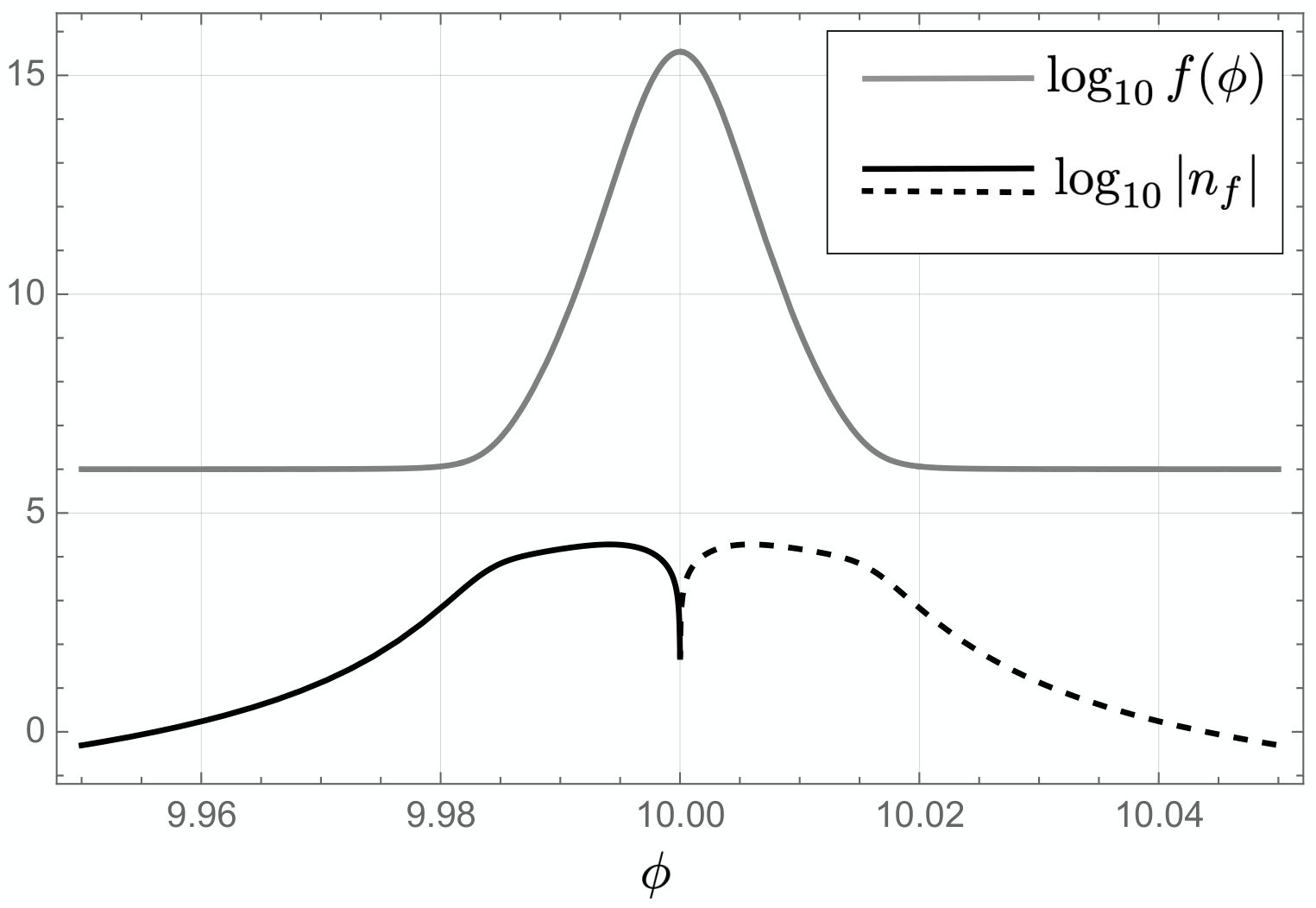
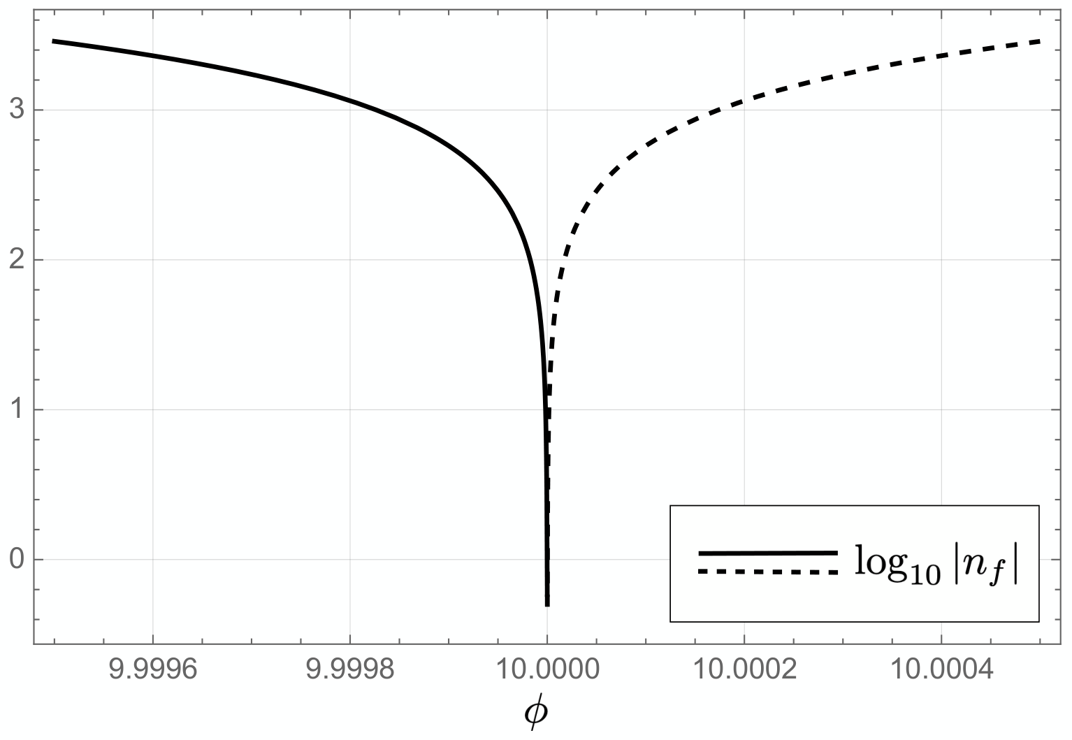
Let us note that the possible physical origins of the presence of a sharp feature in the warp factor have been studied in several articles [15] and we shall not discuss it further. In particular the existence of such features at scales probed by CMB has been studied, however one may consider their presence at smaller energies, not testable by CMB. We shall limit ourselves to analysing its consequences as a possible source of amplification of the curvature perturbations. In order to simplify our model we shall study the consequences of a gaussian feature in an interval with a constant warp factor. Nonetheless one may easily generalise our results to more realistic models.
When the scalar field passes through the region where the feature is present the sound speed decreases and the dynamics may enter a non-canonical phase. Thus, as a consequence, the spectrum of the scalar perturbations gets amplified. One must estimate the duration of such a transient phase and tune the parameters of the model to ensure that the inflaton crosses the feature within a few e-folds. Let therefore consider

$$f=F\left[1+A{\rm e}^{-\frac{\alpha}{{\rm M_{\rm P}}^{2}}(\phi-\phi_{0})^{2}}\right],$$

(41)

where $\alpha^{1/2}$ is inversely proportional to the width of the peak in ${\rm M_{\rm P}}$ units, $\phi_{0}$ is the position of the feature of interest, $A$ is the height of the peak and $F$ is the constant value of the warp factor far away from the peak. While $n_{f}\sim 0$ away from the peak ($|\phi-\phi_{0}|\gg 1$) and in a narrow interval around the peak ($\phi\sim\phi_{0}$) it may grow very large while approaching to $\phi_{0}$. Let us note (see (19) and (20)) that the product $fV\epsilon_{V}$ determines the value of $c_{s}$ during SR inflation. In detail the evolution of the inflaton is described by the following phases:

• i)

  the inflaton slowly rolls toward the peak, $FV\epsilon_{V}\ll 1$ and $c_{s}\simeq 1$; in this phase CMB features are generated;

• ii)

  the inflaton encounters the gaussian feature and climbs. In such a phase if $n_{f}$ is large, $|\dot{\phi}|$ rapidly approaches the value $\sim 1/\sqrt{f}$ (see (23)) and further, If $FAV\epsilon_{V}\gg 1$, the speed of sound is $c_{s}\simeq 0$ (see (22));

• iv)

  the inflaton goes down the peak, $n_{f}$ is large and the speed of sound increases, $c_{s}\rightarrow 1$;

• v)

  the inflaton slowly rolls down the potential until inflation ends.

When the inflaton evolves non-canonically then $|\dot{\phi}|\sim f^{-1/2}$ and

$$\Delta N_{g}=\int_{t_{i}}^{t_{f}}H{\rm d}t=\int_{\phi_{i}}^{\phi_{f}}\frac{H}{\dot{\phi}}{\rm d}\phi$$

(42)

is the number of e-folds needed to cross the (gaussian) feature. Between $\phi_{i}$ and $\phi_{f}$ the gaussian is much larger than $1$ and one has

$$\Delta N_{g}\simeq\int_{\phi_{i}}^{\phi_{f}}\sqrt{\frac{VFA}{3{\rm M_{\rm P}}^{2}}}{\rm e}^{-\frac{\alpha}{2{\rm M_{\rm P}}^{2}}(\phi-\phi_{0})^{2}}{\rm d}\phi\sim\int_{-\infty}^{+\infty}\sqrt{\frac{V_{0}FA}{3{\rm M_{\rm P}}^{2}}}{\rm e}^{-\frac{\alpha}{2{\rm M_{\rm P}}^{2}}(\phi-\phi_{0})^{2}}{\rm d}\phi,$$

(43)

where in the last integral we approximated $V$ by its value at the maximum of the gaussian, $\phi_{0}$, and we extended the integral over the whole real axis because the contributions to the integral from the tails of the gaussian function are negligible. We then obtain the following estimate

$$\Delta N_{g}\sim\sqrt{\frac{2\pi V_{0}FA}{3\alpha}}$$

(44)

which can be expressed in terms of the cosmic time as

$$\Delta t_{g}=\int_{N_{i}}^{N_{f}}\frac{{\rm d}N}{H}\sim\sqrt{\frac{3{\rm M_{\rm P}}^{2}}{V_{0}}}\Delta N_{g}.$$

(45)

Furthermore, close to the maximum of the gaussian $n_{f}$ is $\mathcal{O}\left(1\right)$ and SR is restored.
Let us now evaluate the curvature perturbations spectral amplitude generated by the gaussian feature and compare such an amplitude with that, fixed by observations, at CMB scales. The amplitude of the spectrum generated around $\phi_{0}$, when the inflaton slowly rolls, is given by (36), with $fV\epsilon_{V}\gg 1$, and takes the form

$$\mathcal{P}_{\mathcal{R},0}=\frac{V_{0}}{24\pi^{2}{\rm M_{\rm P}}^{4}}\frac{2f_{0}V_{0}}{3}={\mathcal{P}}_{\mathcal{R}}\frac{2f_{0}V_{0}^{2}\epsilon_{V,*}}{3V_{*}},$$

(46)

where the last equality contains the amplitude ${\mathcal{P}}_{\mathcal{R}}$ at the CMB scales. In order for ${\mathcal{P}}_{\mathcal{R},0}$ to be amplified by $n$ orders of magnitude w.r.t. ${\mathcal{P}}_{\mathcal{R}}$ one then needs

$$\frac{\mathcal{P}_{\mathcal{R},0}}{\mathcal{P}_{\mathcal{R}}}\simeq\frac{2f_{0}V_{0}^{2}\epsilon_{V,*}}{3V_{*}}\sim 10^{n}.$$

(47)

One may also evaluate the spectrum generated by the transient phase before $\phi_{0}$ is crossed, which still occurs for $\phi\sim\phi_{0}$ if the gaussian is sharply peaked around $\phi_{0}$. A rough estimate of (37) on using Eqs. (27,28) leads to $|\gamma|^{2}\sim{\mathcal{O}}(n_{f}^{2}\delta_{1}^{2})$ and

$${\mathcal{P}}_{\mathcal{R},t}\sim\left.\frac{1}{12\pi^{2}}\frac{V_{0}n_{f}^{2}}{\phi_{0}^{2}{\rm M_{\rm P}}^{2}}\right|_{\rm h.e.}\sim\left.\frac{1}{12\pi^{2}}\frac{\alpha V_{0}}{{\rm M_{\rm P}}^{4}}\right|_{\rm h.e.}=\frac{2\alpha V_{0}\epsilon_{V,*}}{V_{*}}{\mathcal{P}}_{\mathcal{R}},$$

(48)

when $n_{f}\gg 1$ and with ${\rm max}\;\left|n_{f}\right|\sim{\mathcal{O}}\left(\phi_{0}{\rm M_{\rm P}}^{-1}\sqrt{\alpha}\right)$. In order for ${\mathcal{P}}_{\mathcal{R},t}$ to be amplified of $n$ orders of magnitude w.r.t. ${\mathcal{P}}_{\mathcal{R}}$ one now needs

$$\frac{\mathcal{P}_{\mathcal{R},t}}{\mathcal{P}_{\mathcal{R}}}\simeq\frac{2\alpha V_{0}\epsilon_{V,*}}{V_{*}}\sim 10^{n}.$$

(49)

In the following sections, using the above expressions, we shall investigate the consequences of the particular choice of the warp factor (41), which for the sake of clarity is plotted in the figure (1), and of the potential.

We finally illustrate a simple applications of our estimates from the previous section and then compare the resulting curvature perturbations spectrum to the numerical (exact) results. For simplicity we consider an exponential potential driving SR inflation

$$V=V_{*}\exp\left[\frac{\beta\left(\phi-\phi_{*}\right)}{{\rm M_{\rm P}}}\right]$$

(50)

with $\beta=3\cdot 10^{-1}$, a constant $\epsilon_{V}=4.5\cdot 10^{-2}$ and a warp factor given by the expression (41). The amplitude (40) fixes

$$V_{*}\sim 2\cdot 10^{-8}{\rm M_{\rm P}}^{4}$$

(51)

and $F$ should be chosen so as to ensure that the sound speed satisfies the experimental constraints. The sound speed must be close to one when CMB scales exit the horizon and therefore we set $F=10^{6}\,{\rm M_{\rm P}}^{-4}$. With such a setup the field slowly rolls down the potential. If we assume that amplification starts $\Delta N_{*}\sim 30$ e-folds after CMB scales exit the horizon one has

$$\phi_{0}\simeq\phi_{*}-\beta^{2}{\rm M_{\rm P}}\Delta N_{*}.$$

(52)

One may therefore estimate (44)

$$\Delta N_{g}\sim\sqrt{\frac{2\pi FV_{*}A}{3\alpha}}\exp\left[-\frac{\beta^{2}\Delta N_{*}}{2}\right]$$

(53)

and the amount of amplification realised during the transient can be related with the parameter $\alpha$ in the gaussian as follows (see (49))

$$\frac{\mathcal{P}_{\mathcal{R},t}}{\mathcal{P}_{\mathcal{R}}}=2\alpha{\rm e}^{-\beta^{2}\Delta N_{*}}\epsilon_{V,*}\sim 10^{n}\Rightarrow\alpha\sim 10^{n+2}.$$

(54)

Near the maximum of the warp factor $f$, SR is restored and the amount of amplification is the following function of the product $F\cdot A$ (see (47))

$$\frac{\mathcal{P}_{\mathcal{R},0}}{\mathcal{P}_{\mathcal{R}}}=\frac{2}{3}FAV_{*}{\rm e}^{-2\beta^{2}\Delta N_{*}}\epsilon_{V,*}\sim 10^{n}\Rightarrow F\cdot A\sim 3\cdot 10^{n+12}.$$

(55)

Let us note that by comparing the ratio of (55) and (54) with (53) one has

$$\frac{\mathcal{P}_{\mathcal{R},0}}{\mathcal{P}_{\mathcal{R},t}}=\frac{FAV_{*}{\rm e}^{-\beta^{2}\Delta N_{*}}}{3\alpha}=\frac{\Delta N_{g}^{2}}{2\pi}$$

(56)

and we therefore observe that for a transient phase lasting ($\sim\Delta N_{g}/2$) few e-folds the two expressions lead to the same amount of amplification.

For more accurate results and in order to test the analytical approximate expressions obtained, a numerical analysis is required.

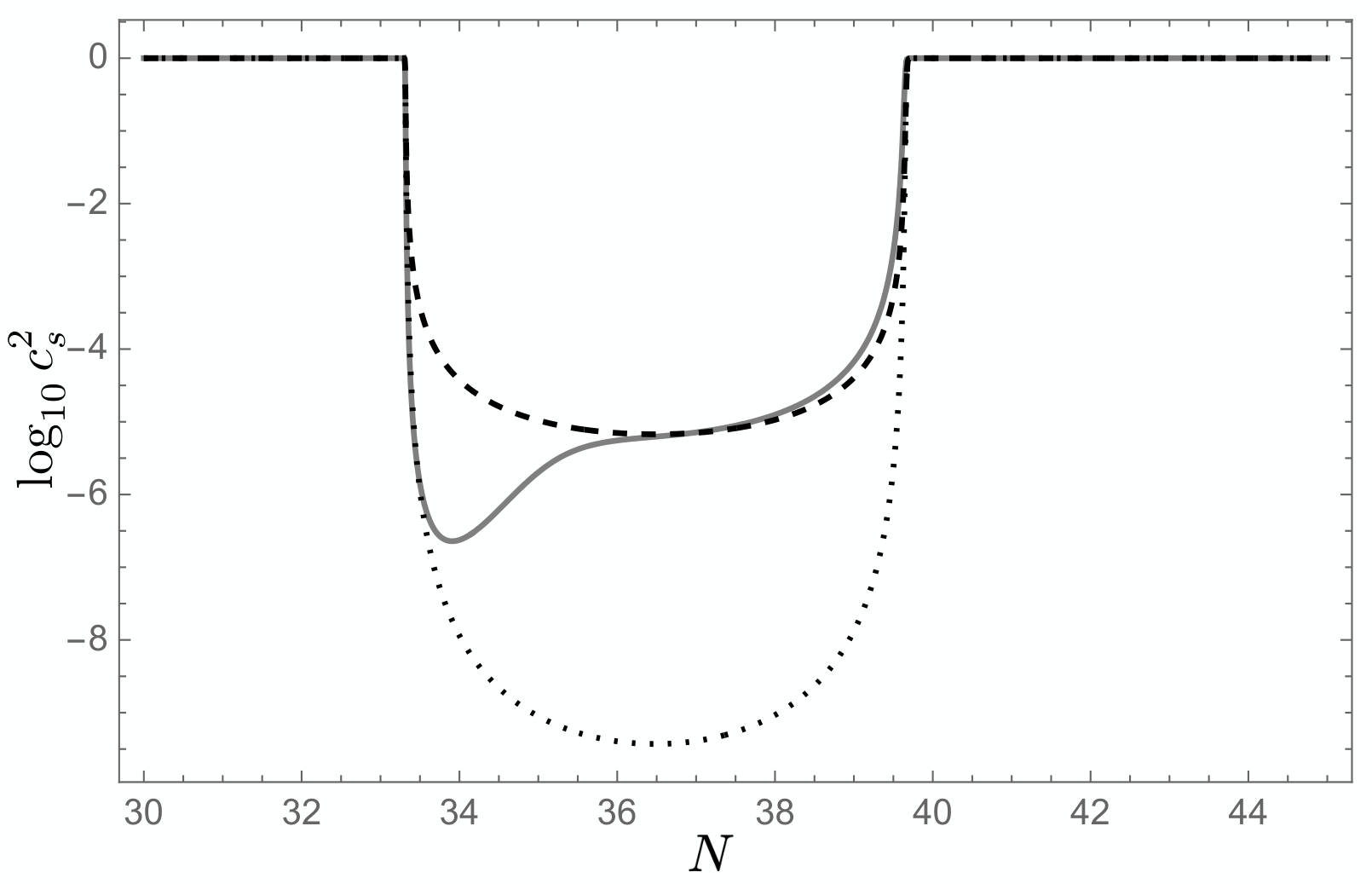
The plot in the figure (2) shows the homogeneous function $\log_{10}c_{s}^{2}$ as a function of $N$ in order to compare the exact (numerical) evolution of the homogeneous system (solid grey line) and the analytical approximations for the SR evolution (dashed line) and the transient (dotted line). The approximations are very close to the exact expression. Let us note that $c_{s}^{2}-1$ is proportional to $f$ which is very large in the interval when the gaussian feature is present and thus $c_{s}^{2}$ is very sensitive to very small differences between the exact and the approximate evolutions. Very small differences between the exact evolution of $\phi(N)$ and the corresponding analytical approximations are amplified by several order of magnitude when multiplied by $f$ and, as the figure shows, result in just a few order of magnitude deviations as far as the evolution of $c_{s}$ is concerned.
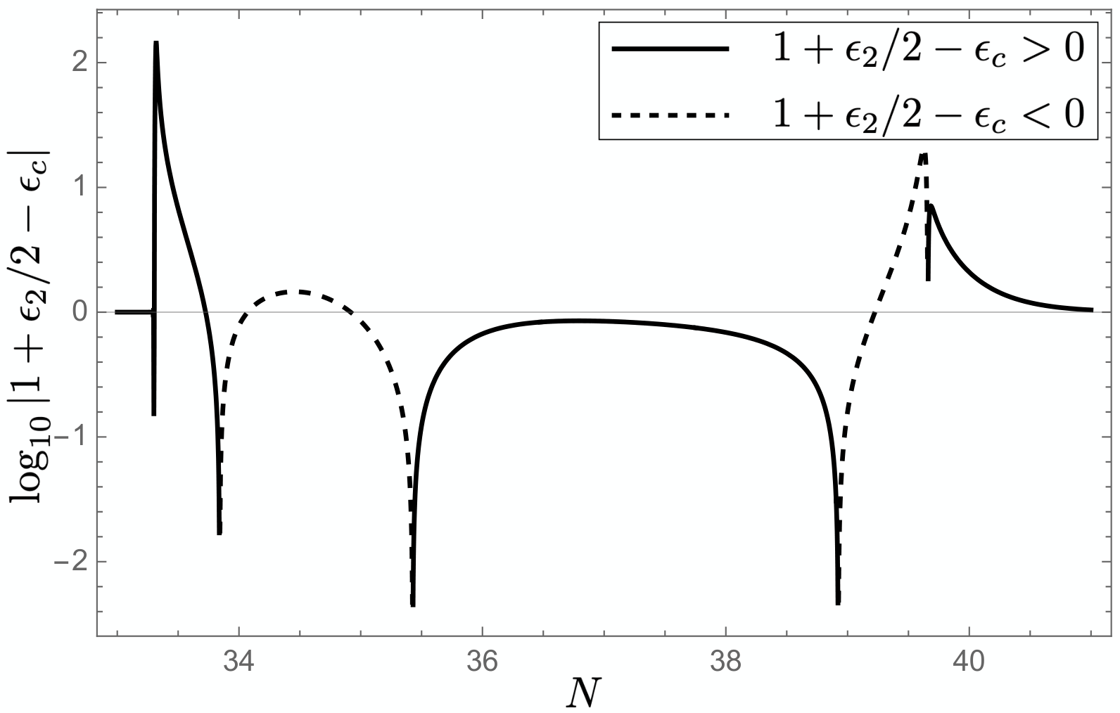
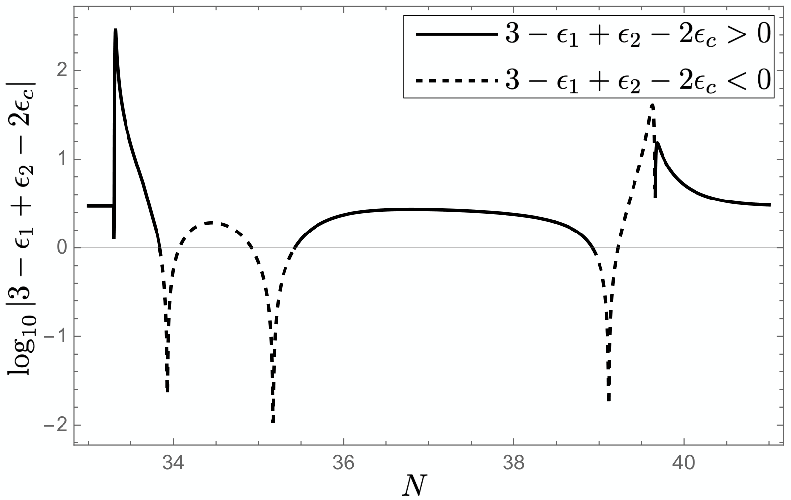
In the figure (3) we plotted two quantities. In the plot on the left the friction term behaviour in Eq. (32) as a function of $N$ is displayed. When the friction is negative (dashed line) the curvature perturbations are amplified. This occurs (roughly) in the two short intervals $N\in[34,35.5]$ and $N\in[39,39.5]$ where the friction term is quite small. The plot on the right illustrates the behaviour of the quantity

$$\xi\equiv 3-\epsilon_{1}+\epsilon_{2}-2\epsilon_{c}$$

(57)

which is associated with the variation of $\mathcal{R}_{k}$ by

$$\frac{{\rm d}\mathcal{R}_{k}}{{\rm d}N}=C_{k}\exp\left[-\int\xi\,{\rm d}N\right].$$

(58)

If SR conditions are satisfied $\xi\sim 3>0$ and ${\rm d}\mathcal{R}_{k}/{\rm d}N\rightarrow 0$ in a few e-folds. Correspondingly $\mathcal{R}_{k}$ freezes. In contrast, in the intervals $N\in[34,35.5]$ and $N\in[39,39.5]$, $\xi$ becomes negative and slightly delays the freezing of $\mathcal{R}_{k}$. Let us note that, while the friction term and $\xi$ become negative for a short amount of time during inflation due to the presence of the gaussian feature in the warp factor, their effect on the total amplification of $\mathcal{R}_{k}$ is still negligible in comparison to that which is originated by the decrease of $c_{s}$ and $\epsilon_{1}$. This fact is confirmed by the numerical estimate of the spectrum on which we shall comment below. In the figure (5) we plotted the spectrum $\log_{10}{\mathcal{P}}_{\mathcal{R}}$ as a function of $\log_{10}k/a_{0}$ and $a_{0}$ is the arbitrary value of the scale factor at the beginning of the numerical analysis. The solid line represents the exact numerical results while the dots corresponds to the analytical estimate (37) evaluated at horizon crossing, where the horizon exit is estimated for each mode by solving exactly the condition $c_{s}k=aH|\gamma|$ through the (homogeneous) exact numerical solutions. We set

$$\alpha\simeq 2.9\cdot 10^{5},\;F=10^{6},\;F\,A\simeq 3.5\cdot 10^{15},$$

(59)

which, according to our estimates, gives an amplification phase of about $\Delta N_{0}\sim 4$ e-folds (it takes $\sim 8$ e-folds for the scalar field to get across the gaussian feature) and an amplification factor of about $3$ orders of magnitude.
Let us note that (37) well approximates the numerical results before and after the transient stage and when the field enters in the region where $|n_{f}|$ becomes large ($c_{s}$ decreases) at the onset of the gaussian feature. Close to the maximum of $f$ the homogeneous evolution enters a short SR phase and finally $|n_{f}|$ becomes large again ($c_{s}$ increases) as the field crosses the maximum of the gaussian feature and finally relaxes on the SR attractor with $f={\rm const}$. The figure shows that after the first large variation of $f$ the amplitude ${\mathcal{P}}_{\mathcal{R}}$ reaches a maximum and then begins oscillating with an increasing frequency. This oscillation is the consequence of modes re-entering the horizon due to the increasing speed of sound. At the horizon re-entry $v_{k}$ evolves as a superposition of ingoing and outgoing waves

$$v_{k}\sim\frac{1}{\sqrt{2c_{s}k}}\left[C_{k}{\rm e}^{i\int_{\eta_{k}}^{\eta}kc_{s}{\rm d}\eta^{\prime}}+D_{k}{\rm e}^{-i\int_{\eta_{k}}^{\eta}kc_{s}{\rm d}\eta^{\prime}}\right],$$

(60)

where $\eta_{k}$ is the conformal time at re-entry, and therefore its modulus oscillates. Let us note that at early times, before exiting the horizon for the first time, the Bunch-Davies initial condition sets $D_{k}\rightarrow 0$ for each mode and modulus oscillations are absent. At the end of inflation, the amplitude of the modes outside the horizon is frozen and the oscillation remains imprinted in the perturbations.
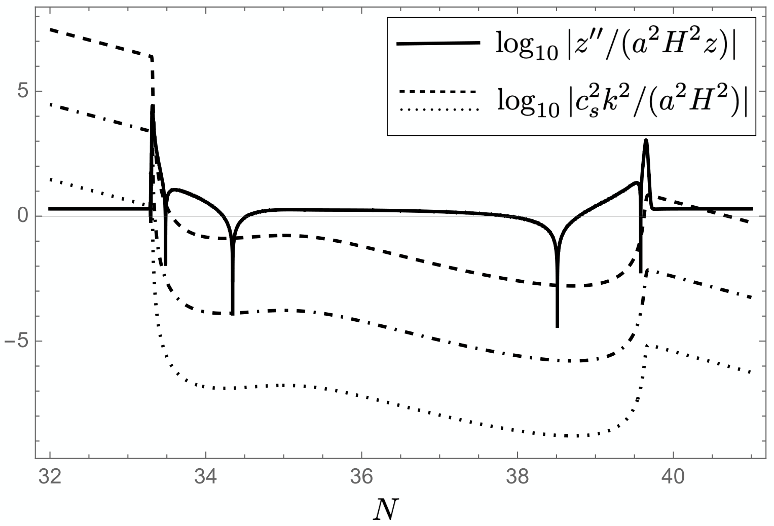
In the figure (4) we plotted the two contributions in the time dependent frequency of the Mukhanov-Sasaki equation (29) rescaled by $a^{2}H^{2}$. When $k^{2}c_{s}^{2}\gg|z^{\prime\prime}/z|$ the modes are “inside” the horizon and oscillate; in contrast when $k^{2}c_{s}^{2}\ll|z^{\prime\prime}/z|$ the modes are “outside” the horizon and the curvature perturbations evolve according to (33). If $k\,c_{s}$ slowly evolves monotonically and $z^{\prime\prime}/z$ rapidly increases monotonically (as in common inflationary models) the two regimes are sequential for each mode. For the case under study, as Fig. (4) shows, a certain bunch of perturbation modes may cross the horizon several times (see for example the dashed line which finally “exits the horizon” at $N\sim 41$). The resulting effect for this bunch of modes is that they are in a superposition of the form (60) before the last “horizon exit” and an oscillatory region of the spectrum is generated. Let us note that the oscillation is more evident if $|C_{k}|\sim|D_{k}|$ in (60). The modes which do not belong to the above subset just cross the horizon once and the resulting part of spectrum shows no evident oscillation.

The amplification realised with the choice of parameters (59) is just an example of how the presence of a sharp feature in the warp factor may affect the scalar power spectrum at the end of inflation. The example shows that the analytical estimates of the previous sections are quite consistent. A suitable choice of $\alpha$, $F$ and $A$ will certainly lead to an amplification of 6-7 orders of magnitude, eventually resulting in PBHs formation with a mass depending on $\Delta N$ (38). We restricted our analysis to the study of a few order of magnitude of amplification because a precise numerical analysis and a much steeper warp factor needed by a much larger amount of amplification would have required too much time and processor power.
Let us finally note that our results can be easily generalised to different potentials and warp factors. In particular, the steepness required to obtain a large amplification in a short amount of time needs a very localised feature and is therefore very mildly sensitive to the global form of $f$ and $V$. Lastly we observe that models with a varying speed of sound has been discussed in the literature since in the regime with $c_{s}\ll 1$ a significant amount of non-gaussianities can be generated [16]. The common estimates for the abundance of PBHs generated as a consequence of the amplification of the curvature perturbations during inflation assume a gaussian distributed amplitude for such perturbations. The existence of possibly large deviations from gaussianity has been very debated in the literature [nongauss] and, although no general consensus has been found, it is still widely believed that non-gaussianities may improve the efficiency of PBHs formation with a much smaller amount of perturbations amplification.
Furthermore, the third order contributions to the action for the perturbations $\mathcal{R}(x)$ include interactions with couplings which are inverse proportional to $c_{s}^{2}$ and may therefore be non-perturbative when $\mathcal{R}(x)$ is large enough and $c_{s}^{2}$ is small. This fact is relevant in particular if one considers effective theories of inflation, defined below a given energy scale, and whose quantum corrections explode for $c_{s}^{2}$ below a certain threshold. Let us note, that such terms are multiplied by time derivatives of $\mathcal{R}$ and, for modes which freeze after the horizon exit, the contribution are therefore suppressed, in contrast with the cases where the amplification is generated by a non-negligible $\dot{\mathcal{R}}$ as a consequence of a negative friction term.
This question is certainly important but its solution is far from being obvious due to the consequences of non-gaussianities themselves and other details involved in the collapse which are often glossed over but significantly affect the efficiency of PBHs formation. Let us stress, however, that this article only discusses the details of a mechanism for amplification of curvature perturbations in the context of DBI inflation which is supposed to be valid within the linear regime and neglecting the cubic/higher order interactions. If the validity of the linear approximation do not allow for an amplification large enough to generate $100\%$ of PBHs DM, still one may consider the consequences of a smaller amplification phase, leading to a smaller, but significant, amount of PBHs.

References

- [1] B. P. Abbott et al. [LIGO Scientific and Virgo], Phys. Rev. Lett. 116 (2016) no.6, 061102 doi:10.1103/PhysRevLett.116.061102 [arXiv:1602.03837 [gr-qc]].
- [2] Y. B. ;. N. Zel’dovich, I. D., Soviet Astron. AJ (Engl. Transl. ), 10 (1967), 602; S. Hawking, Mon. Not. Roy. Astron. Soc. 152 (1971), 75
- [3] G. F. Chapline, Nature 253 (1975) no.5489, 251-252 doi:10.1038/253251a0; P. Meszaros, Astron. Astrophys. 38 (1975), 5-13
- [4] A.A. Starobinsky. Springer. in H.J. De Vega and N. Sanchez (eds.) Current trends in field theory quantum gravity and strings, Lecture Notes in Physics 246 Verlag, Heidelberg, 1986), pp. 107-126. A.D. Linde. Academic. Particle Physics and Inflationary Cosmology (Harwood New York, 1990).
- [5] V.F. Mukhanov, Sov. Phys. JETP 68, 1297 (1988); J. M. Maldacena, JHEP 0305 (2003) 013; V. F. Mukhanov, H. A. Feldman and R. H. Brandenberger, Phys. Rept. 215 (1992) 203. V.F. Mukhanov, Phys. Lett. B 218, 17 (1989); J. M. Bardeen, Phys. Rev. D 22, 1882 (1980). doi:10.1103/PhysRevD.22.1882 M. Sasaki, Prog. Theor. Phys. 70 (1983) 394. doi:10.1143/PTP.70.394
- [6] B. J. Carr, Astrophys. J. 201 (1975) 1. doi:10.1086/153853 M. Sasaki, T. Suyama, T. Tanaka and S. Yokoyama, Class. Quant. Grav. 35 (2018) no.6, 063001 doi:10.1088/1361-6382/aaa7b4 [arXiv:1801.05235 [astro-ph.CO]].
- [7] J. Garcia-Bellido and E. Ruiz Morales, Phys. Dark Univ. 18 (2017) 47 doi:10.1016/j.dark.2017.09.007 [arXiv:1702.03901 [astro-ph.CO]]. G. Ballesteros and M. Taoso, Phys. Rev. D 97 (2018) no.2, 023501 doi:10.1103/PhysRevD.97.023501 [arXiv:1709.05565 [hep-ph]]. M. Cicoli, V. A. Diaz and F. G. Pedro, JCAP 1806 (2018) no.06, 034 doi:10.1088/1475-7516/2018/06/034 [arXiv:1803.02837 [hep-th]]. H. Motohashi and W. Hu, Phys. Rev. D 96 (2017) no.6, 063503 doi:10.1103/PhysRevD.96.063503 [arXiv:1706.06784 [astro-ph.CO]]. C. Germani and T. Prokopec, Phys. Dark Univ. 18 (2017) 6 doi:10.1016/j.dark.2017.09.001 [arXiv:1706.04226 [astro-ph.CO]].
- [8] M. Born and L. Infeld, Proc. Roy. Soc. Lond. A 144 (1934) no.852, 425-451 doi:10.1098/rspa.1934.0059 M. Alishahiha, E. Silverstein and D. Tong, Phys. Rev. D 70 (2004), 123505 doi:10.1103/PhysRevD.70.123505 [arXiv:hep-th/0404084 [hep-th]]; D. Bessada, W. H. Kinney and K. Tzirakis, JCAP 09 (2009), 031 doi:10.1088/1475-7516/2009/09/031 [arXiv:0907.1311 [gr-qc]]. W. H. Kinney and K. Tzirakis, Phys. Rev. D 77 (2008), 103517 doi:10.1103/PhysRevD.77.103517 [arXiv:0712.2043 [astro-ph]]. M. Spalinski, Phys. Lett. B 650 (2007), 313-316 doi:10.1016/j.physletb.2007.05.041 [arXiv:hep-th/0703248 [hep-th]].
- [9] C. Armendariz-Picon, T. Damour and V. F. Mukhanov, Phys. Lett. B 458 (1999) 209 doi:10.1016/S0370-2693(99)00603-6 [hep-th/9904075]. J. Garriga and V. F. Mukhanov, Phys. Lett. B 458 (1999) 219 doi:10.1016/S0370-2693(99)00602-4 [hep-th/9904176]. R. Gwyn, M. Rummel and A. Westphal, JCAP 1312 (2013) 010 doi:10.1088/1475-7516/2013/12/010 [arXiv:1212.4135 [hep-th]]. P. Franche, R. Gwyn, B. Underwood and A. Wissanji, Phys. Rev. D 81 (2010) 123526 doi:10.1103/PhysRevD.81.123526 [arXiv:0912.1857 [hep-th]].
- [10] O. Özsoy, S. Parameswaran, G. Tasinato and I. Zavala, JCAP 07 (2018), 005 doi:10.1088/1475-7516/2018/07/005 [arXiv:1803.07626 [hep-th]].
- [11] A. Y. Kamenshchik, A. Tronconi, T. Vardanyan and G. Venturi, Phys. Lett. B 791 (2019), 201-205 doi:10.1016/j.physletb.2019.02.036 [arXiv:1812.02547 [gr-qc]].
- [12] B. Carr and F. Kuhnel, Ann. Rev. Nucl. Part. Sci. 70 (2020), 355-394 doi:10.1146/annurev-nucl-050520-125911
- [13] P. A. R. Ade et al. [Planck Collaboration], arXiv:1502.02114 [astro-ph.CO]. P. A. R. Ade et al. [Planck Collaboration], arXiv:1502.01589 [astro-ph.CO]. Y. Akrami et al. [Planck Collaboration], arXiv:1807.06211 [astro-ph.CO]. N. Aghanim et al. [Planck Collaboration], arXiv:1807.06209 [astro-ph.CO].
- [14] J. M. Maldacena, JHEP 0305 (2003) 013 doi:10.1088/1126-6708/2003/05/013 [astro-ph/0210603]. N. Bartolo, E. Komatsu, S. Matarrese and A. Riotto, Phys. Rept. 402 (2004) 103 doi:10.1016/j.physrep.2004.08.022 [astro-ph/0406398]. G. Franciolini, A. Kehagias, S. Matarrese and A. Riotto, JCAP 1803 (2018) no.03, 016 doi:10.1088/1475-7516/2018/03/016 [arXiv:1801.09415 [astro-ph.CO]]. P. A. Klimai and E. V. Bugaev, arXiv:1210.3262 [astro-ph.CO]. V. Atal and C. Germani arXiv:1811.07857 [astro-ph.CO] X. Chen, M. x. Huang, S. Kachru and G. Shiu, JCAP 0701 (2007) 002 doi:10.1088/1475-7516/2007/01/002 [hep-th/0605045]. J. Noller and J. Magueijo, Phys. Rev. D 83 (2011) 103511 doi:10.1103/PhysRevD.83.103511 [arXiv:1102.0275 [astro-ph.CO]].
- [15] V. Miranda, W. Hu and P. Adshead, Phys. Rev. D 86 (2012), 063529 doi:10.1103/PhysRevD.86.063529 [arXiv:1207.2186 [astro-ph.CO]]. R. Bean, X. Chen, G. Hailu, S. H. H. Tye and J. Xu, JCAP 03 (2008), 026 doi:10.1088/1475-7516/2008/03/026 [arXiv:0802.0491 [hep-th]]. V. Miranda and W. Hu, Phys. Rev. D 89 (2014) no.8, 083529 doi:10.1103/PhysRevD.89.083529 [arXiv:1312.0946 [astro-ph.CO]]. V. Miranda and W. Hu, Phys. Rev. D 89 (2014) no.8, 083529 doi:10.1103/PhysRevD.89.083529 [arXiv:1312.0946 [astro-ph.CO]]. T. Kobayashi and J. Yokoyama, JCAP 02 (2013), 005 [erratum: JCAP 09 (2013), E02] doi:10.1088/1475-7516/2013/02/005 [arXiv:1210.4427 [astro-ph.CO]].
- [16] G. Ballesteros, J. Beltran Jimenez and M. Pieroni, JCAP 06 (2019), 016 doi:10.1088/1475-7516/2019/06/016 X. Chen, M. x. Huang, S. Kachru and G. Shiu, JCAP 01 (2007), 002 doi:10.1088/1475-7516/2007/01/002 M. A. Gorji, H. Motohashi and S. Mukohyama, [arXiv:2110.10731 [hep-th]].