An active learning approach for improving the performance of equilibrium based chemical simulations
Abstract.
In this paper, we propose a novel sequential data-driven method for dealing with equilibrium based chemical simulations, which can be seen as a specific machine learning approach called active learning. The underlying idea of our approach is to consider the function to estimate as a sample of a Gaussian process which allows us to compute the global uncertainty on the function estimation. Thanks to this estimation and with almost no parameter to tune, the proposed method sequentially chooses the most relevant input data at which the function to estimate has to be evaluated to build a surrogate model. Hence, the number of evaluations of the function to estimate is dramatically limited. Our active learning method is validated through numerical experiments and applied to a complex chemical system commonly used in geoscience.
Key words and phrases:
machine learning, Gaussian Process, chemical simulations1. Introduction
Computing the concentrations at equilibrium of reactive species is well known to be a challenging issue when the number of species is high and/or when the reaction involves the dissolution or the precipitation of minerals [22, 18, 3]. The numerical resolution of these non-linear problems can quickly become so time consuming that the coupling with other physical processes has to be simplified. For instance in the case of reactive transport, it means that the size of the geometric model has to be drastically limited leading typically to a one dimensional model or that the number of time steps has to be reduced. To overcome this issue, research efforts have been dedicated to the improvement of the numerical scheme aiming at speeding up the computations. A classical approach consists in using a splitting operator technique to solve separately the transport of the chemical species and the chemical reaction between those species [12, 19, 4, 2, 17]. With this approach a specific optimization for each part of the resolution can be performed especially by taking advantage of the parallel architecture of computers [5, 7, 8].
However, despite the significant improvements of the numerical solvers and preconitionners during the last decades, three dimensional large scale modelling of complex reactive transport over a long period of time, namely many time steps, remains almost impossible to solve with standard computers. Consequently, the recent success of machine learning (ML) in various fields have quickly drawn attention of geoscientists because ML seems to be able to solve very complex problems with a reasonable cost in terms of computational ressources.
The main idea behind the ML success is to provide an estimation of the solution of the full simulation model that can replace it. Two of the most popular approaches are model order reduction and data-driven models also called surrogate models. The first one requires to understand the underlying chemical processes to create a simplified model while preserving some physical principles [14]. In the second approach, the underlying chemical processes are not assumed to be known or understood and a model is solely built from a limited but potentially significant set of values of the solution of the full simulation model associated to some specific input values [9]. Since the number of required values is unknown a priori, choosing the optimal input values and parameters used for building the surrogate model is crucial and usually challenging.
In this paper, we propose a novel sequential data-driven method for dealing with equilibrium based chemical simulation, which can thus be seen as an active learning approach inspired by the ideas contained in [20, 10]. With such an approach, our goal is to minimize the number of evaluations of the function that has to be estimated to build a surrogate model. Our approach consists in modeling the function to estimate as a sample of a Gaussian Process (GP) which allows us to provide an error estimation to sequentially choose the most relevant input data until a given stopping criterion is fulfilled. The advantage of our approach is that the number of required evaluations of the function to estimate is very limited and that there are no parameter to tune.
The paper is organized as follows. In Section 2, our approach is described. Some numerical experiments are provided in Section 3 to illustrate the statistical and numerical performance of our method. It is then applied in Section 4 to a multidimensional example coming from [11] which includes several chemical elements and minerals.
2. Description of our approach
In this section, we describe our active learning approach for estimating a real-valued function defined on a compact subset by using only a few number of sequentially well-chosen points at which is evaluated.
We adopt a Bayesian point of view which consists in considering as a sample of a zero-mean Gaussian process (GP) having a covariance function that we shall denote by GP(0,) in the following. The advantage of this approach is that, conditionally on a set of observations where , belonging to , the posterior distribution is still a GP having a mean and a covariance function given by
| (1) | ||||
| (2) |
where . Here ′ denotes the matrix transposition, and are in and , where the ’s are in . For further details on GP, we refer the reader to [15] in which their properties are thoroughly presented.
In our case, models a physical quantity that is assumed to be smooth, so for our applications we shall consider two covariance functions that are commonly used in this case. The first one is the squared exponential (SE) covariance function
| (3) |
| (4) |
Here the hyperparameters are the characteristic length scales. Actually, these hyperparameters can be understood as how far you need to move along a particular axis in the input space so that the function values become uncorrelated. For further details, we refer the reader to Section 5.1 of [15]. Note that Definition (3) allows us to model anisotropic response surfaces.
As explained in [15], since this covariance function is infinitely differentiable, the GP with this covariance function has mean square derivatives of all orders. As argued by [21] such strong smoothness assumptions may be unrealistic for modeling many physical processes, so we shall also consider another covariance function belonging to the Matérn class of covariance functions defined by
| (5) |
where is a modified Bessel function with Bessel order , see [1, Section 9.6], and is defined by
| (6) |
being defined in (4). In this situation, as explained in [15], the GP is -times mean-square differentiable if and only if . Here, we shall focus on the case where , for which has a computationally advantageous expression. Indeed, for , where is in ,
| (7) |
with defined in (6); see [1, Equation 10.2.15] for further details.
In the following, we shall denote by A a fine grid of :
| (8) |
This grid is either a regular grid of when is small (usually 1 or 2) or a Latin Hypercube Sampling for larger values of . Note that this grid contains the points at which the estimation of is performed and that the points at which is evaluated are chosen in this grid.
Inspired by [20] who proposed a sequential approach for maximizing a function by modeling it using a Gaussian process, we propose a strategy which consists in adding the new point to the set of observations at which needs to be evaluated as follows:
| (9) |
where
| (10) |
being defined in (2) and being the set of where reaches its maximum. Note that the points at which needs to be evaluated are chosen in the fine grid of defined in (8).
2.1. Estimating the characteristic length scales
Previously, we assumed that the characteristic length scales were known. However, this is obviously not the case in real-data applications. We propose using the maximum-likelihood strategy described in [15] to estimate . This adds a step to the method previously described, as the ’s have to be estimated before evaluating the posterior distribution of the GP using (1) and (2). Hence, for the observation set with , the posterior log-likelihood given by:
| (11) |
with and , has to be maximized with respect to .
2.2. Summary of our strategy
Our method was implemented by using the GaussianProcessRegressor class of the scikit-learn 0.20.3 module of Python which only provides the computation of and defined in (1) and (10). Our sequential approach is summarized in Algorithm 1.
Input: a small initial set of points of where has been evaluated
; Choose a covariance function among SE and Matérn.
While the stopping criterion is not fulfilled
The function is estimated by defined in (1).
Further comments on the stopping criteria appearing in Algorithm 1 are given below.
2.3. Stopping criteria
Different stopping criteria based on the following quantities can be used.
- •
Ratio variance. At each iteration of our method, the following average is computed:
(12) where is defined in (10) and , or . This criterion will be then compared to a threshold to determine if the maximal variance reach a plateau. In some cases, can be less than so in order to detect the smallest variations, we also have to make sure that the ratio does not exceed the inverse of the chosen threshold. Thus, the associated stopping criterion is: interrupt the algorithm when is such that
(13) - •
Mobile average. At each iteration of our method, the following average is computed:
(14) for or where is defined in (10). The associated stopping criterion is: interrupt the algorithm when is such that
(15) - •
Maximal variance. At each iteration of our method,
(16) is computed where is defined in (10). The associated stopping criterion is: interrupt the algorithm when is such that
(17) where or 0.001 in the following.
The statistical performance of these different criteria are investigated in Section 3. Note that the values reported here for each criteria (, or ) were chosen based on some numerical experiments since they appear to be relevant to detect a plateau in the maximal variance.
3. Numerical experiments
To illustrate our method we consider hereafter the estimation of the amount of a "Salt" mineral as a function of the concentrations of its constituents Sp and Sp. For this example, the thermodynamic constants of the halite salt (NaCl) were considered because there are only two constitutive elements and because they do not depend on the pH of the solution. From our point of view, there is no theoretical limitation in the application of our method to more complex salts or minerals.
Following the law of mass action, the dissolution reaction of this mineral writes:
At equilibrium, the activity of these elements a and a obey the solubility product
The amount of Salt was first calculated with PHREEQC [13] as a function of the concentrations of Sp, which is normalized so that . It corresponds to the case below. The corresponding function is displayed in the left part of Figure 1 where is a regular grid of with points. Then, the amount of Salt was computed with PHREEQC as a function of the concentrations of Sp and Sp, which are also normalized so that . It corresponds to the case below. The corresponding function is displayed in the right part of Figure 1 where is a regular grid of with points.

3.1. Case
The different steps of our approach summarized in Algorithm 1 are illustrated in Figure 2 where our procedure was arbitrarily stopped after evaluations. Here, we used the SE covariance function defined in (3).
The approach starts with points randomly chosen in . Then, a new point in green is added to the set of points at which an evaluation of is required. This point corresponds to the position on the -axis where the uncertainty associated to the estimation of is maximized. We can see from this figure which displays the true function , the estimation of and the points at which has been evaluated that evaluation points are enough to obtain a very accurate estimation of .
To further investigate the statistical performance of our approach, we used the following measures:
| (18) |
where is the estimation of obtained at iteration , is the number of elements in the grid A and and are the minimum and maximum values, respectively, found for the evaluation of on the initial grid ;
| (19) |
| (20) |
where is defined in (10).
The average and the standard deviation of these measures obtained from 10 replications of the initial set of points are displayed in Figure 3 for the covariance functions defined in (3) and (7) and . Note that the average and the standard deviation are computed by using 10 different initial sets of points.
We can see from this figure that the performance of our approach is slightly better for the Matérn covariance function than for the squared exponential function. It can indeed reach a normalized MAE (resp. normalized sup norm) of (resp. ) by using only 40 evaluations of the function to estimate. This might come from the discontinuity of the first derivative of the function to estimate where the salt starts to precipitate.
In the left part of Figure 4 the statistical performance of our approach including the stopping criteria are further investigated thanks to the computation of the previous performance measures defined in (18), (19) and (20): , and where is the stopping iteration which may be different for each stopping criterion.
We can see from the left part of Figure 4 that among all of the stopping criteria, “ratio variance 5” (), “ratio variance 10” () and “mobile average 10” () are those providing the best estimations of the function . Moreover, we can observe from the right part of this figure that our active learning approach only requires between 15 and 40 evaluations of the function to estimate instead of the 1140 points of the initial grid to provide a very accurate estimation of the function . With such an approach, we can thus expect a significant reduction of the computational time especially in situations where the computational load associated to the evaluation of is high. Figure 4 also shows that, in this case, the impact of the covariance function is not significant even though the first derivative of the function to approximate is not continuous, namely where the salt precipitates.
3.2. Case
In order to further assess the performance of our approach we now consider the estimation of the amount of Salt as a function of the concentrations of Sp and Sp.
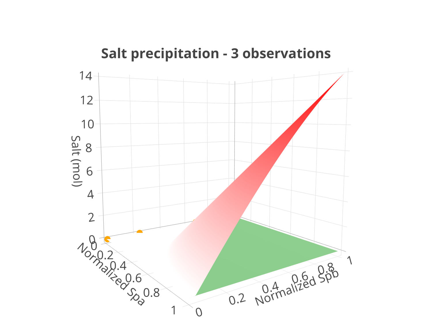
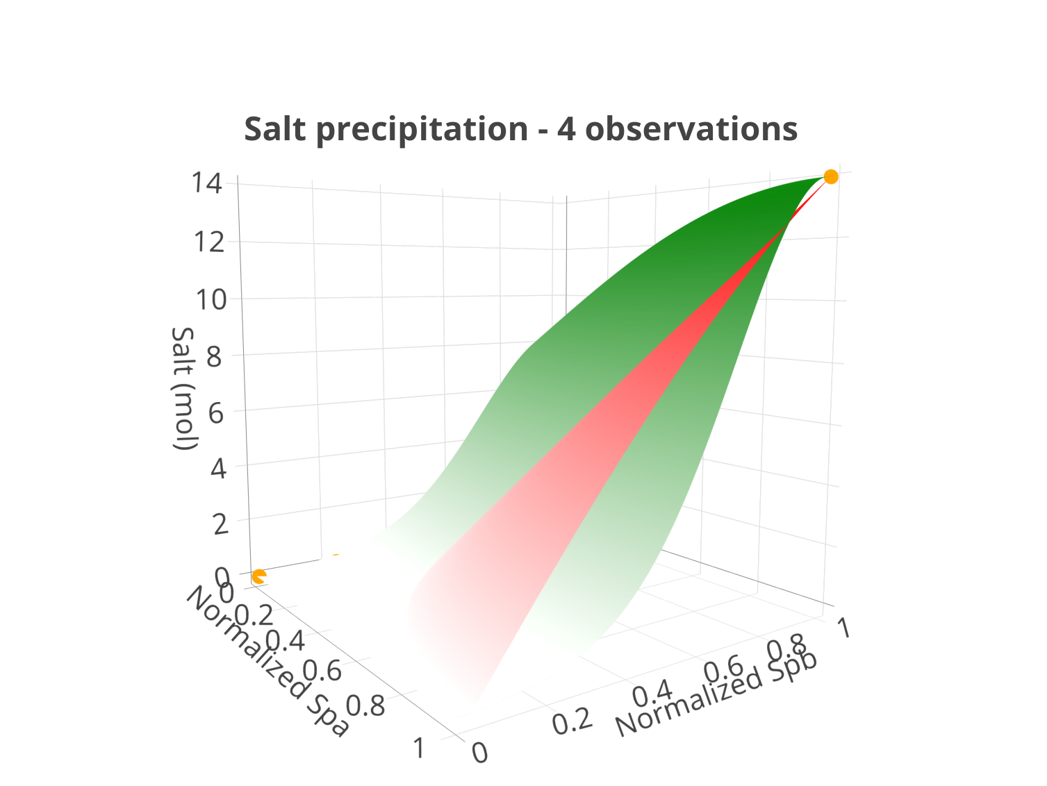
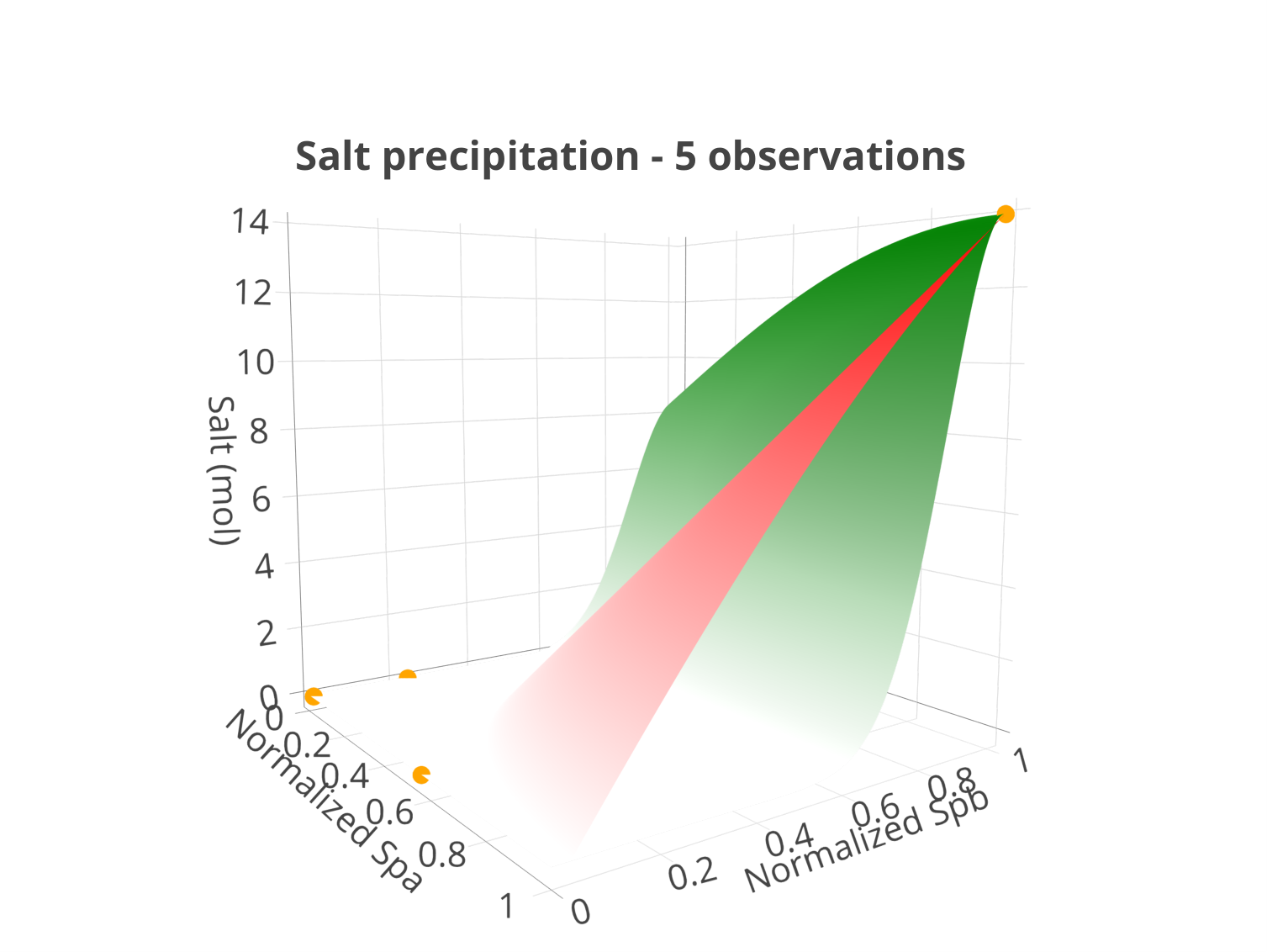
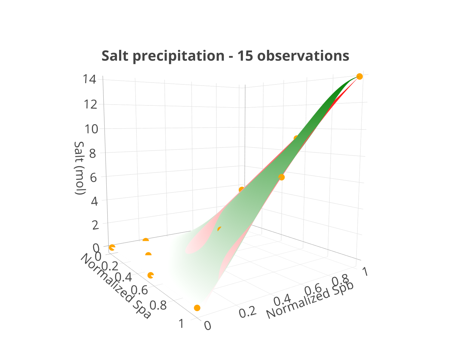
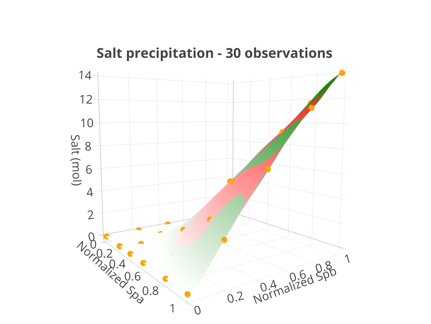
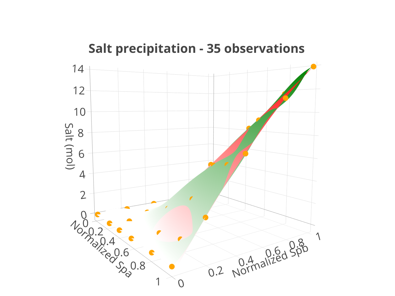
The different steps of our approach summarized in Algorithm 1 are illustrated in Figure 5. Here, we used the SE covariance function defined in (3).
The approach starts with points randomly chosen in obtained thanks to a regular grid of points. Then, new points (orange bullets) are added one by one to the set of points at which an evaluation of is required. These points correspond at each iteration to the position in where the uncertainty associated to the estimation of is maximized. We can see from this figure which displays the true function , the estimation of and the points at which has been evaluated that 35 evaluation points are enough to obtain a very accurate estimation of .

In the case, the average and the standard deviation of the statistical measures defined in (18)–(20) obtained from 10 replications of the initial set of points are displayed in Figure 6 for the squared exponential and the Matérn covariance function defined in (3) and (7)) for . We can see that for both choices of covariance function the performance of our approach are similar: it can reach a normalized sup norm (resp. normalized MAE) of (resp. ) by using only evaluations of the function to estimate instead of the 40000 points of the grid A. We also observe a smoother behavior of the maximal variance with the Matérn covariance function even though the final values are close.
We can see from the left part of Figure 7 that most of the stopping criteria provide an accurate estimation of the function except “ratio variance 2” (). As for the case, the stopping criteria and provide very satisfactory results. Moreover, we can observe from the right part of this figure that thanks to our active learning approach, 30-50 evaluations of the function to estimate are required instead of the 40000 points of the initial grid to provide a very accurate estimation of the function . Once again, with our approach, we can thus expect a significant reduction of the computational burden especially in situations where the computational load associated to the evaluation of is high.
In this case, the choice of the covariance function might result from a trade-off between accuracy and number of evaluation points. However, the accuracy and the number of evaluation points do not change drastically suggesting that the choice of the covariance function is still not significant.
4. Application to a multidimensional geochemical system
The chemical problem solved in this section derives from [11]. The chemical setup is based on the thermodynamic data for aqueous species and minerals available in the Phreeqc.dat database distributed with PHREEQC [13]. The compositional system actually solved consists of 14 species in solution, 2 mineral components, 8 geochemical reactions and 2 mineral dissolution-precipitation reactions:
Then, each amount of mineral (calcite or dolomite, respectively) is computed with PHREEQC [13] as a function of the total elemental concentrations (C, Ca, Cl, Mg), the pH (as )) and the mineral amount (dolomite or calcite, respectively), which are normalized so that . Here, our goal is to estimate the functions and defined as follows:
| (21) |
by using the minimal number of evaluations of these functions. For this, we shall use a grid built thanks to a Latin Hypercube Sampling (LHS) of with points.
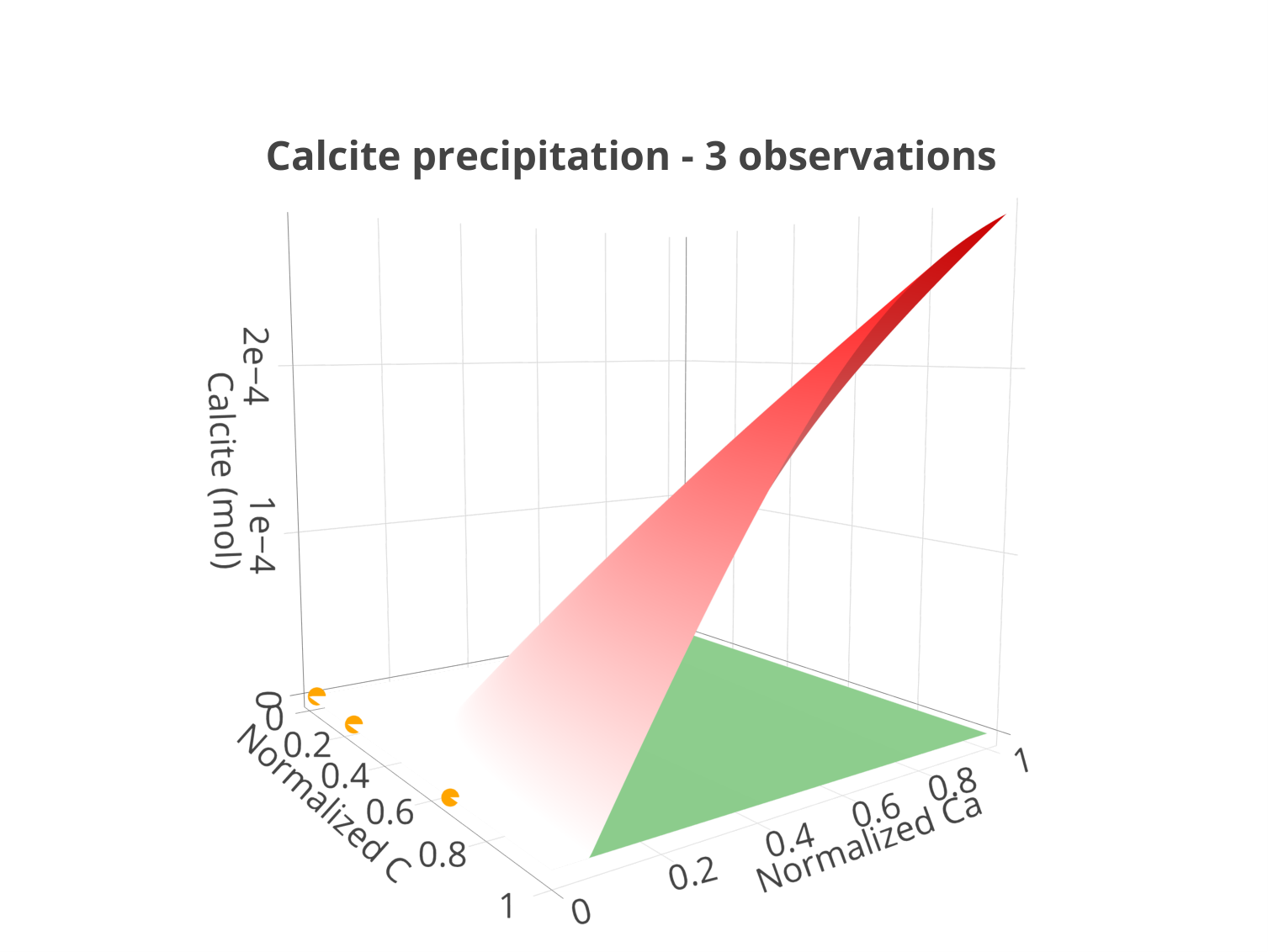
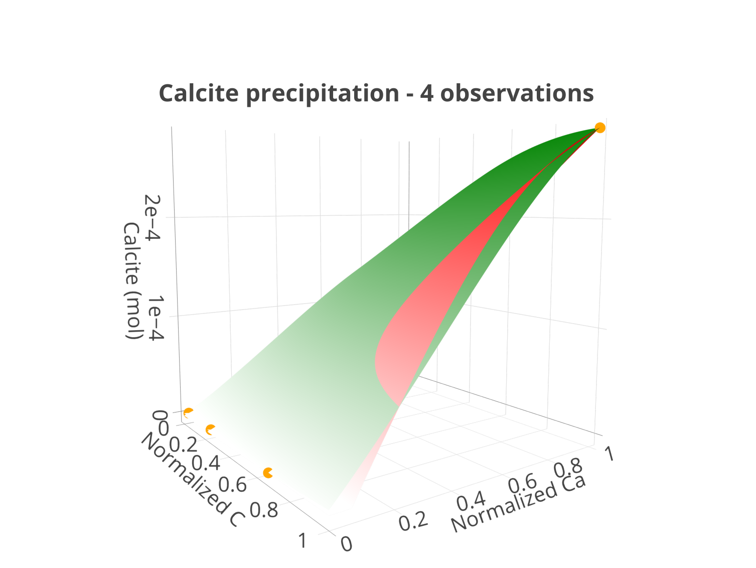
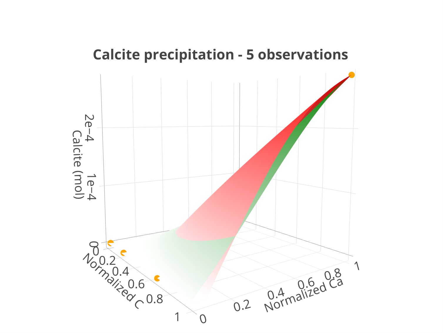
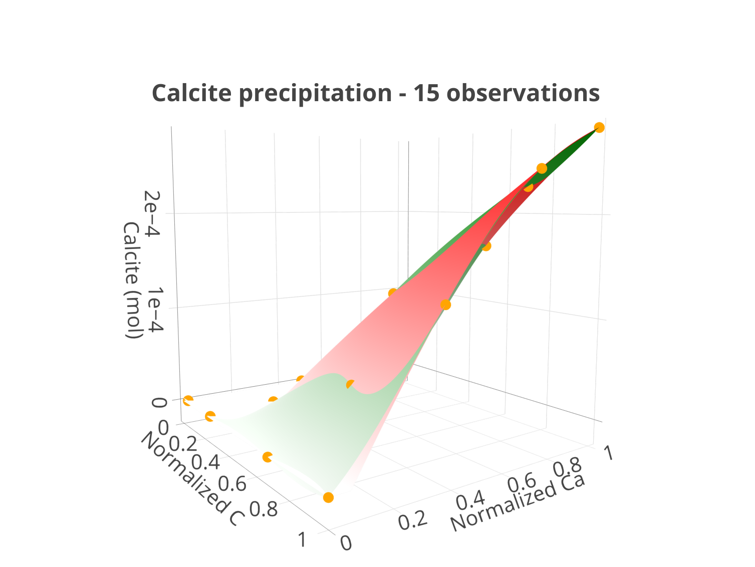
In the left part of Figure 8 the amount of calcite is displayed as a function of C and Ca for Cl= mol/kgw, Mg= mol/kgw, pH=10, dolomite=0 mol which corresponds to . In the right part of Figure 8 the amount of dolomite is displayed as a function of Ca and Mg for C=5 mol/kgw, Cl= mol/kgw, pH=10, calcite=0 mol which corresponds to .
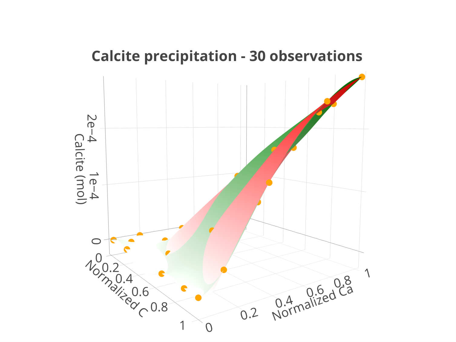
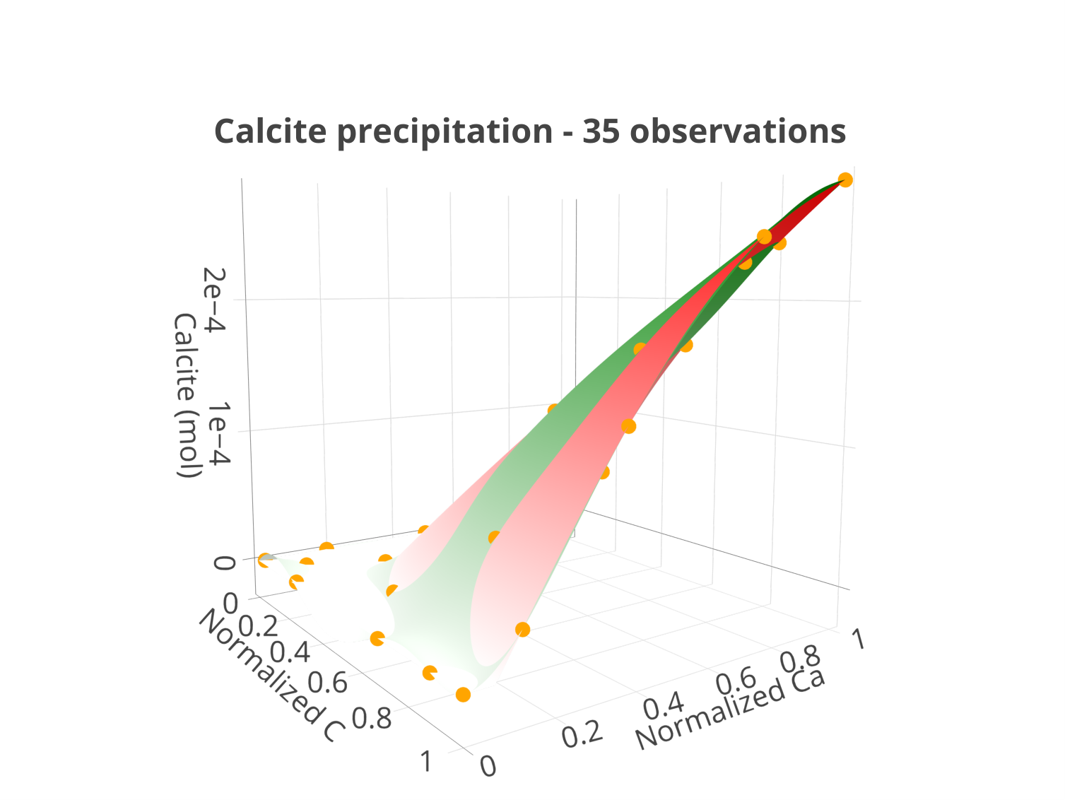
Illustrations of our active learning approach for estimating these functions are shown in Figures 13 and 14 of the Appendix.


4.1. Calcite precipitation
The average and the standard deviation of the different statistical measures obtained from 10 replications of the initial set of points are shown in Figure 9 for the squared exponential and the Matérn covariance functions defined in (3) and (7) for . We can see that for both choices of covariance functions, the maximal variance and the statistical precision measures keep decreasing as the number of evaluations increases. For instance, our method allows us to have a normalized sup norm (resp. normalized MAE) of (resp. ) with only 500 evaluations instead of the 100 000 points of the grid A for both covariance functions. However, the maximal variance is around (resp. ) for the squared exponential (resp. Matérn) covariance function.
Moreover, we can see from Figure 10 that when the mobile average criteria and the squared exponential covariance function are used the final estimation of is obtained with around 100 evaluations of instead of . To obtain similar statistical performance with the Matérn covariance more than 750 observations are required. The difference between the two covariance functions probably comes from the behavior of the maximal variance. It is still strongly decreasing after 500 observations for the squared exponential covariance function which is not the case for the Matérn covariance function.
4.2. Dolomite precipitation
Similarly to the previous case, the average and the standard deviation of the different statistical measures obtained from 10 replications of the initial set of points are shown in Figure 11 for the squared exponential and the Matérn covariance functions defined in (3) and (7) for . We obtained similar conclusions as for the calcite precipitation case, see Figure 12.
5. Conclusion
We have shown that our method has two main features which make it very attractive. Firstly, it is very efficient from a practical point of view thanks to the Gaussian Process modeling which enables us to sequentially build the surrogate model with a low number of points and almost no parameters to tune. Secondly, its very low computational burden makes its use possible on complex chemical reactions involving singular behaviors like precipitation and dissolution of minerals. Our method could also be applied to more complex geochemical systems like surface complexation or ion exchange that can be described with laws of mass action. Effectively, these two features have further potential applications on much larger sets of reactive species or with coupled physical processes namely in reactive transport modeling. This will be the subject of a future work.
References
- [1] M. Abramovitz and I. Stegun. Handbook of Mathematical Functions with Formulas, Graphs and Mathematical Tables. Dover books on mathematics. Dover Publications, 1965.
- [2] J. Carrayrou, R. Mosé, and P. Behra. Operator-splitting procedures for reactive transport and comparison of mass balance errors. Journal of Contaminant Hydrology, 68(3-4):239–268, 2004.
- [3] C. de Capitani and T. H. Brown. The computation of chemical equilibrium in complex systems containing non-ideal solutions. Geochimica et Cosmochimica Acta, 51(10):2639–2652, 1987.
- [4] S. Descombes. Convergence of a splitting method of high order for reaction-diffusion systems. Mathematics of Computation, 70(236):1481–1501, 2001.
- [5] I. Faragó and J. Geiser. Iterative operator-splitting methods for linear problems. International Journal of Computational Science and Engineering, 3(4):255–263, 2007.
- [6] A. Forrester, A. Sobester, and A. Keane. Engineering design via surrogate modelling: a practical guide. Wiley, 2008.
- [7] J. Geiser. Iterative splitting methods for differential equations. Taylor & Francis Group: Boca Raton, FL, USA; London, UK; New York, NY, USA, 2011.
- [8] J. Geiser, J. L. Hueso, and E. Martínez. Parallel iterative splitting methods: Algorithms and applications. In AIP Conference Proceedings, volume 2293, page 420081. AIP Publishing LLC, 2020.
- [9] D. Guérillot and J. Bruyelle. Geochemical equilibrium determination using an artificial neural network in compositional reservoir flow simulation. Computational Geosciences, 24(2):697–707, 2020.
- [10] M. Jala, C. Levy-Leduc, Éric Moulines, E. Conil, and J. Wiart. Sequential design of computer experiments for the assessment of fetus exposure to electromagnetic fields. Technometrics, 58(1):30–42, 2016.
- [11] O. Kolditz, U.-J. Görke, H. Shao, and W. Wang. Thermo-hydro-mechanical-chemical processes in porous media: benchmarks and examples, volume 86. Springer Science & Business Media, 2012.
- [12] G. Marchuk. Splitting and alternating direction methods. volume 1 of Handbook of Numerical Analysis, pages 197–462. Elsevier, 1990.
- [13] D. L. Parkhurst and C. Appelo. Description of input and examples for phreeqc version 3: a computer program for speciation, batch-reaction, one-dimensional transport, and inverse geochemical calculations. U.S.G.S. Techniques and Methods, book 6, chap. A43, 497p., 2013.
- [14] S. Rao, A. van der Schaft, K. van Eunen, B. M. Bakker, and B. Jayawardhana. Model-order reduction of biochemical reaction networks. In 2013 European Control Conference (ECC), pages 4502–4507. IEEE, 2013.
- [15] C. E. Rasmussen and C. K. I. Williams. Gaussian Processes for Machine Learning (Adaptive Computation and Machine Learning). The MIT Press, 2006.
- [16] J. Sacks, W. J. Welch, T. J. Mitchell, and H. P. Wynn. Design and analysis of computer experiments. Statistical Science, 4(4):409–423, 1989.
- [17] M. J. Simpson and K. A. Landman. Analysis of split operator methods applied to reactive transport with monod kinetics. Advances in Water Resources, 30(9):2026–2033, 2007.
- [18] W. R. Smith. The computation of chemical equilibria in complex systems. Industrial & Engineering Chemistry Fundamentals, 19(1):1–10, 1980.
- [19] B. Sportisse. An analysis of operator splitting techniques in the stiff case. Journal of computational physics, 161(1):140–168, 2000.
- [20] N. Srinivas, A. Krause, S. Kakade, and M. Seeger. Information-theoretic regret bounds for Gaussian process optimization in the bandit setting. IEEE Information Theory, 58:3258–3265, 2012.
- [21] M. L. Stein. Interpolation of spatial data. Springer Series in Statistics. Springer-Verlag, 1999.
- [22] W. B. White, S. M. Johnson, and G. B. Dantzig. Chemical equilibrium in complex mixtures. The Journal of Chemical Physics, 28(5):751–755, 1958.
6. Appendix: Additional plots