Compressive Independent Component Analysis: Theory and Algorithms
Abstract
Compressive learning forms the exciting intersection between compressed sensing and statistical learning where one exploits forms of sparsity and structure to reduce the memory and/or computational complexity of the learning task. In this paper, we look at the independent component analysis (ICA) model through the compressive learning lens. In particular, we show that solutions to the cumulant based ICA model have particular structure that induces a low dimensional model set that resides in the cumulant tensor space. By showing a restricted isometry property holds for random cumulants e.g. Gaussian ensembles, we prove the existence of a compressive ICA scheme. Thereafter, we propose two algorithms of the form of an iterative projection gradient (IPG) and an alternating steepest descent (ASD) algorithm for compressive ICA, where the order of compression asserted from the restricted isometry property is realised through empirical results. We provide analysis of the CICA algorithms including the effects of finite samples. The effects of compression are characterised by a trade-off between the sketch size and the statistical efficiency of the ICA estimates. By considering synthetic and real datasets, we show the substantial memory gains achieved over well-known ICA algorithms by using one of the proposed CICA algorithms. Finally, we conclude the paper with open problems including interesting challenges from the emerging field of compressive learning.
Keywords Independent Component Analysis Compressive Learning Sketching Compressive Sensing Summary Statistics Cumulants
1 Introduction
In recent years, the size of datasets have grown exponentially as a result of advances in technology, signal acquisition, and the sophistication of modern day mobile phones and devices. This has enabled researchers, statisticians and machine learning practitioners to build increasingly accurate models as a consequence of larger sample sizes and feature dimensions. Nevertheless, this poses a fundamental challenge to large scale learning as (i) traditional algorithms have computational complexity that scales with the order of the dataset dimensions (ii) the whole dataset has to be stored or transferred on to local RAM as optimisation methods need to return to the data (or a random subset of the data) at subsequent iterations, and (iii) one is vulnerable to malicious attacks of potentially sensitive and personal information as the data needs to be stored or transferred locally. Compressive learning (CL) [1, 2] partially addresses these fundamental challenges by severely compressing the whole dataset into a random representation of fixed size, named a so-called sketch, in a single (or limited) pass of the data prior to learning. Once the sketch is formed, the parameters of the model are inferred solely from the sketch, hence a CL algorithm, for a given task or model, needs never to return to the original dataset, and it can be deleted from memory as a result. At the core of the CL framework [1, 3], is that in general, the size of the sketch does not scale with the dimensions of the dataset, or indeed the data’s underlying dimensionality, but instead is driven by the complexity or dimensionality of the task or model of interest. In theory, one can work with datasets of arbitrary length, as the dimension of the sketch is fixed constant throughout, making CL especially amenable to large scale learning. Inferring the parameters of a model solely from the sketch is an under determined inverse problem. As a result, we need regularity assumptions to make the problem well-posed. These assumptions come in the form of a low dimensional model set that the solution to the inference problem lies on or close to. The reader may notice this is reminiscent of compressive sensing where one assumes the signal of interest is sparse in some domain, and therefore the solution lies on or close to the union of dimensional subspaces representing a low dimensional model set. The sparse regularity assumption allows one to take a limited number of measurements to recover the signal of interest and reduce the complexity and cost of acquisition. In later sections, we take inspiration from compressive sensing to develop and analyse our CL algorithms.
In this paper, we develop a CL framework, including theory and practical algorithms, for independent component analysis (ICA). ICA is an unsupervised learning task that attempts to find the linear transformation that separates some given data into components of maximal independence. It is used extensively in the machine learning and signal processing communities for example as a dimensionality reduction tool [4], to uncover underlying factors that effect the price movements of a collection of stocks [5] and to detect independent sources in the brain through EEG signals [6]. As will be discussed in section 2, the ICA problem can be solved directly from the data or through some higher order statistics of the data, such as the kurtosis. Given that the number of independent sources is denoted by and the signal or data length is denoted by , then the memory complexity typically scales either with or depending on the method of choice. As one can see, this becomes infeasible for large scale datasets. In this paper, we show theoretically and empirically that it is possible to design a CL ICA algorithm where the sketch dimension, and therefore the memory complexity, scales at which can be orders of magnitudes smaller than current approaches.
1.1 Contributions and Outline
Below, we highlight the main contributions of the paper:
- •
Focusing on the higher order statistics method of ICA, we show that an independent component model set exists in the space of order cumulant tensors and we state the set’s dimensionality.
- •
We prove that the well-known restricted isometry property (RIP) holds for projections of the cumulant tensor on the model set with a sketch size , which is order optimal to the dimensional of the model set. Given a sketch constructed from random Gaussian ensembles, we show that the reconstruction error is stable when measuring a signal which lives close to, but not on, the ICA model set through the existence of an instance optimal decoder.
- •
Two inherently different CICA algorithms are proposed, in the form of an alternating steepest descent and an iterative projection gradient algorithm and show that they successfully recover the ICA mixing matrix with overwhelming probability provided that the sketch size . We analyse the proposed CICA algorithms on synthetic and real datasets showing that the CICA scheme achieves substantial memory savings over existing ICA methods, whilst retaining competitive estimation accuracy.
- •
We analyse the tradeoff between the compression rate of the sketch and the overall statistical efficiency of the sketch estimate.
1.2 Related Works
1.2.1 Existing Compressive Learning Models
The framework of CL has been successfully applied to a host of learning tasks and models with the desired outcome of reducing the complexities associated with signal acquisition, computation and memory storage. In [3], Keriven et al. proposed a CL framework for mixture models, in particular the mixture of Gaussian distributions and -means learning tasks. In both cases, a sketch is constructed by randomly sampling the characteristic function of the mixture model which can be equivalently seen as taking random Fourier features of the data [7]. The compact representational sketch of each mixture model scales as , where is the number of mixtures in the model and is the feature space dimensions of the data. As a result, a compressive mixture model algorithm was proposed that had both computational and space complexities that scaled independently of the number of data points . In [1], a compressive principal component analysis (PCA) framework was proposed. As will be discussed in Section 2.2, the compressive PCA methodology is aligned closely to our compressive ICA framework. Distinct from compressive mixture models, the compressive PCA method is left distribution free and it is assumed that the data lives on, or can be approximately modelled, by a -dimensional subspace. As a result, a sketch of size can be computed by taking a random projection of the covariance matrix of the data, hence reducing the memory complexities of storing either the data of size or the covariance matrix of size .
1.2.2 Generalised Method of Moments
Compressive learning is similar to the technique of Generalised Method of Moments (GeMM) [8, 9] where the parameters of interest are estimated by matching a collection of generalised moments of the distribution with the empirical counterparts calculated through the data. In most cases it is used instead of maximum likelihood estimation when calculating the likelihood is not tractable. CL differs from much of the GeMM literature as the goal is fundamentally different: in compressive learning one attempts to construct a compact representation of data with the aim of reducing complexity constraints (computation, memory, acquisition) whilst in GeMM the goal is to primarily estimate when the model is either partially specified or the likelihood does not have a closed form solution. Moreover, the selected generalised moments may be a function of the parameter being estimated, hence not providing a one off sketch.
1.2.3 Streaming Methods
Closely related to CL is the collection of streaming methods [10, 11], where data items are seen and queried only once by the user and then discarded. This is of particular interest when the summary statistic of choice is updated and maintained in real time, for example in the online learning setting [12], to reduce space complexities. Notably, the count-min-sketch [13] was developed to query data in an online fashion with the application of maintaining histograms of quantiles. However, these methods in general focus on the discrete collection of objects and database queries while in CL the framework and method is applied to machine learning tasks where typically the signal is question is continuous. Tropp et al. [14] proposed a streaming framework for large scale PCA. In particular, in [11], the authors design random sketches for on-the-fly compression of data matrices associated with large scale scientific simulations. Here the data matrix of interest can be decomposed into a sequence
| (1) |
where it is assumed each has some structural redundancies for example sparsity or low-rank. These methods have a subtle yet fundamental difference from CL, as in CL the structural assumptions which are exploited to form the CL sketch arise from the model or distribution itself, while in these streaming methods the structural assumptions come directly from the data. Moreover, several passes of the data may be required to reduce the low-rank approximation error [14].
1.2.4 Other Compression Techniques
Coresets are a popular method used to compress a database into a summary statistic used for inferring the parameters of a given model and has been used primarily for subspace clustering based tasks [15, 16]. In a similar vein to CL, the compact data representation has size that typically scales independently to the number of input items and the dimension of input feature space. However, the coresets are constructed in a hierarchical manner, possibly resulting in multiple passes of the data and are therefore not naturally amenable to online or distributed learning. Projections that include both random projections and feature selections [17, 18] are used widely to reduce the dimensionality of the data. In [18], datasets were randomly projected into a compressed domain using both random Gaussian and Bernoulli matrices. In a similar vein to compressive sensing [19], the data was assumed to be -sparse therefore the dependency of the feature space dimension was removed within the space and acquisition complexities. In contrast to random projections, more structural based projections are proposed. In [20], different feature selection techniques for classification are reviewed including structured graph methods and the use of embedded models. The well-known PCA method is a popular preprocessing technique that projects the dataset onto a -dimensional subspace of maximal variance [21]. In both random and structured projections, the methods discussed only tackle the dependency of the feature space dimension and do not address the challenges posed by a large data size . Sub-sampling methods are also a popular method for dimensionality reduction whereby a subset of the original dataset is used for learning. As discussed previously, the method of coresets [15, 16] is a sub-sampling technique that attempts to sub-select dominant items that well approximate the structure of the dataset. Other sub-sampling techniques include random and adaptive sub-sampling [10]. The disadvantage of sub-sampling techniques is that there is a risk of discarding important information relating to non-sampled data items. Moreover, these techniques only tackle the constraint on the number of data items and don’t combat the complexity issues posed by the feature space dimensional .
Specifically to ICA compression, Sela et al. [22] used kernel approximation techniques to reduce the dimensions of the Kernel ICA method proposed by Bach [23]. Random Fourier features are used to approximate the kernel, reducing the memory complexity from to , where is the number of random Fourier weights used. Despite the reduction in memory complexity, the algorithm still has storage demands which scale linearly with . In comparison, we remove the dependency of the data length completely, within our framework, when estimating the ICA mixing matrix.
2 Background
2.1 Compressive Learning
Let be independent and identically distributed samples from an unknown probability distribution on where is some Euclidean space and is a Borel -field. Classically, is parametrized by some parameters denoted by . A statistical learning problem can be formalised as follows: find a hypothesis from a hypothesis class that best matches the probability distribution over the training collection , given some data fidelity term. Given a loss function , this is equivalent to minimizing the risk defined as
| (2) |
Formally, the model set associated to the hypothesis class can be defined as:
| (3) |
In other words, the set containing all distributions for which zero risk is achievable. As a result, the model set has a dimension which is intrinsic to the hypothesis class of the model. In practice, one cannot minimize the true risk as we generally do not have access to the true distribution , so instead, one can minimize the empirical risk with respect to the finite samples of the true distribution and as a result this may mean all the data is required to be stored in memory.
In CL [3, 1, 2], we find a compact representation, or a so-called sketch, that encodes some statistical properties of the data. Its size is ideally chosen relative to the intrinsic complexity of the problem, making it possible to work with arbitrarily large datasets while storing in memory an object of fixed size. Given a feature function , such that is integrable with respect to any , define a linear operator by
| (4) |
The sketch defined in (4) can be seen as taking the expectation of some particular features of the distribution , which is similar to the field of kernel mean embedding [24] where one uses feature maps to embed probability distributions. Therefore, we would like to construct so that captures sufficiently relevant information of the data to allow us to infer the parameters of the model directly from the sketch. As a trivial example, if we seek to infer only the mean of a normal distribution , the construction where would constitute a trivial yet sufficient sketch. In reality, CL is applicable to much more complex models where the feature function is non-trivial and the model may not necessarily possess a finite dimensional sufficient statistic independent from the data. The goal of CL is to therefore construct a sketch of size that captures enough information to recover an estimated risk which is close to the true risk with high probability [1]. In practice, as in the kernel mean embedding literature [24], the empirical distribution is used to form an empirical sketch defined as
| (5) |
denoting by the Dirac distribution on , and therefore the empirical sketch can be formed directly from the data. Due to the law of large numbers, . Once the sketch has been computed, one can discard the dataset from memory. As a result, CL reduces down to solving an inverse problem of the form
| (6) |
where is a cost function designed for the specific learning task at hand. In a compressive sensing light, we can exploit structural assumptions of the model set and the associated parameter space , e.g sparsity, low rankness, low dimensional manifold properties, to make (6) well-posed and finding a solution tractable. As such, one can design a decoder that exploits the structural assumptions of the model set to recover the parameters of the model from the sketch whilst minimizing the risk. The sketching operator and the decoder form the pair that define the CL algorithm for a specific learning problem. It should be noted that minimizing (6) plays the role of a proxy for minimizing the empirical risk as, by definition of the model set in (3), any has zero loss in expectation [1].
| Learning Task | - Means | GMM | PCA |
|---|---|---|---|
| Model set | |||
| Feature func. | |||
| Sketch cost | s.t | ||
| Sketch Size |
2.2 Compressive Principal Component Analysis
In Section 2.1, the framework of CL was discussed in a general manner without specific consideration of the distributional form of the model. As will be discussed in Section 2.3, the PCA and ICA models are similar in nature in that the model is often left distribution free. In other words, the distribution of the sampled data is left unspecified. In Table 1, it is shown that the compressive PCA model set [1] is defined as
| (7) |
Due to the distribution free assumption of the PCA model, we seek structural assumptions that are manifested within some intermediary statistic space to make computing a sketch possible [25]. In the case of compressive PCA, the space of covariance matrices is leveraged as an intermediary statistic space where the rank of the covariance matrices is exploited. Figure 1 depicts a geometric viewpoint of both compressive parametric learning (e.g. -means, GMM) and distribution free compressive learning (e.g. PCA, ICA). In general, distribution free CL poses distinct challenges and advantages from the typical parametric CL framework [26]. Challenges arise when choosing an intermediary statistic space , for instance (1) what set of intermediate statistics can we use? (2) How do the structural assumptions of the model set manifest within the intermediate statistic? Equivalently, there are many advantages. Specifically, by leveraging some set of intermediate statistics we have implicitly mapped the problem from an infinite dimensional probability space to a typically finite dimensional statistic space. As a result, we can utilise a host of existing techniques within the compressive sensing literature to design encoder and decoder pairs . Moreover, it also allows us to use a more flexible semi-parametric model that is only partially specified. As will be discussed in Section 4, the compressive ICA framework follows a similar convention where the space of 4th order cumulant tensors is used as an intermediary statistic space to exploit structural assumptions of the model set to form a sketch.

2.3 Independent Component Analysis
ICA is used frequently in the machine learning and signal processing communities to identify latent variables that are mutually independent to one another. Consider a data vector , then the problem of ICA concerns finding a mixing matrix (here we assume that ) such that
| (8) |
where and the components are statistically independent:
| (9) |
The data point is only one realisation of a data matrix or signal of length , so therefore we attempt to infer with the collective set of linear equations , where is a realisation of . There are many techniques and methods in the literature to solve the ICA problem. The simplest method is to assume the distributional form of each of the independent components and then solve the ICA problem through a maximum likelihood approach [27]. In practice, the distributions are not known a-priori so therefore in most methods the distributions are left unspecified. As a result, practitioners and researchers often resort to minimizing a given contrast function to solve the ICA problem.
2.3.1 Prewhitening
A popular preprocessing trick for ICA is to prewhiten the data beforehand. This involves the process of finding the matrix such that
| (10) |
where has identity covariance matrix. This initial preprocessing step, which can be executed through singular value decomposition based techniques, uncorrelates the mixed components and handles the issue of when there are more mixing components than independent components . Moreover, it has the advantage that the matrix to be found is necessarily orthogonal and square. For the sake of presentation, we will subsequently consider the whitened version of the data for the remainder of this section and the corresponding whitened ICA equation
| (11) |
In Section 4.3, we propose 2 equivalent sketching frameworks that can either incorporate prewhitened and unwhitened data.
2.3.2 Cumulant Based ICA
Tensorial or cumulant based methods are a group of techniques used to solve the ICA problem and are of particular interest in this paper. Statistical properties of the data instance can be described by its cumulants . In the multivariate setting, cumulants give rise to tensors, denoted for a cumulant tensor of order . Assuming the data has zero mean, the first four cumulants are defined [28] as
| (12) | ||||
where is the expectation operator. Given the model in (11) equating to , then the following multilinear property holds for their associated cumulant tensors:
| (13) |
where represents the -mode tensor-matrix product and represents the order cumulant tensor of the independent source signals [28]. In this paper we will only consider order cumulant tensors (e.g. ) and for the sake of simplified notation we shall drop the superscript in (13) for the rest of the discussion. We denote by the space of 4th order cumulant tensors which account for the symmetry in (12), where each cumulant tensor has a maximum of unique entries (degrees of freedom) [29]. The diagonal entries are the auto-cumulants of , while the off-diagonal entries are the cross-cumulants. If the variables are statistically independent then, as seen by (12), the cross-cumulants vanish to 0 resulting in a strictly diagonal cumulant tensor. In other words, independence implies diagonality. It is shown in [30] that under mild conditions the converse is also true, i.e. diagonality implies independence. Cumulant based ICA can therefore be seen as finding a linear transformation such that the resulting cumulant tensor
| (14) |
is strictly diagonal. We can define the following ICA model set:
| (15) |
where is the set of diagonal cumulant tensors, defined formally as
| (16) |
Here, we have the additional requirement11 1 A standard requirement in ICA is that at maximum one diagonal cumulant can be zero which arises from the ICA assumption that at maximum one source signal is Gaussian [4]. Here we have the slightly stronger assumption that all source signals are non-gaussian. that each diagonal cumulant is greater than or equal to a small constant . The expected cumulant tensor is typically not known owing to finite data length approximations and non-Gaussian additive noise [31] and so in general cannot be fully diagonalized by a linear transform. As a result, contrast functions are used to approximately diagonalize and maximize the independence of the system.
2.3.3 Contrast Functions
A contrast function is a mapping from the space of distributions to the real line and is a measure of the statistical independence between latent variables in a linear system [32, 4]. For a function to be a contrast function it must be permutation and scaling invariant, and also maximized if and only if the distributions are statistically independent [32]. For instance, the negative mutual information satisfies the contrast conditions, although it can be difficult to estimate in practice. Typically, contrast functions are tractable approximations of information theoretical measures such as negative mutual information, maximum likelihood and negentropy. Comon proposed various cumulant based contrast functions in [32], that are Edgeworth expansions of information theoretic measures. The simplest is given by
| (17) |
where is the order cumulant tensor corresponding to the variable . When is maximum, the components of are independent giving and . A 4th order cumulant tensor that has a decomposition as given in (14) and is therefore a member of the model set, , maximizes any given cumulant based contrast function [32], and hence minimizes the associated information theoretic measure and the risk in (2). For further details, comprehensive reviews of cumulants and tensors can be found in [32, 28].
As discussed in Section 2.2, the 4th order cumulant tensor will act as an intermediary statistic space (). It is well documented through identifiability results in the cumulant based ICA literature [32, 31] that the parameters of the ICA model, namely the mixing matrix , can be estimated solely from the 4th order cumulant tensor. As such, the 4th order cumulant tensor can be seen in its own right as a sketch, albeit inefficient with respect to compression being . In the next section, we motivate the principles behind sketching the 4th order cumulant tensor to form a compact representational sketch that has size .
3 Compressive Learning Principles for Cumulant ICA
It was discussed in Section 2.3.2 that the model set of the ICA problem defined in (15), maximizes any given cumulant based contrast function [32]. The model set is itself a low-dimensional space residing in the space of cumulant tensors . Specifically, can be described as the product set of the set of orthogonal matrices, denoted , and the set of diagonal cumulant tensors that was defined in (14). We can therefore initially count the degrees of freedom of the model set :
- •
- A maximum of degrees of freedom on the leading diagonal.
- •
- A maximum of degrees of freedom [33].
In total, the model set has degrees of freedom. In comparison, the space of 4th order cumulant tensors , in which the model set resides, has degrees of freedom. As the model set is of low complexity, in principle we could form a sketch of the 4th order cumulant tensor and estimate the parameters of the ICA model, namely the mixing matrix , solely from the sketch. The sketch of the 4th order cumulant tensor is defined by
| (18) |
where w denotes that the sketch is acting on the whitened data . The computation of the sketch is very related to the sketching method of compressive PCA highlighted in Table 1. Akin to compressive PCA, the sketching operator acts on the finite dimensional space of 4th order cumulant tensors instead of the infinite dimensional probability space which is left unspecified due to the nature of the ICA model. The ICA sketch defined in (18) draws strong connections to finite dimensional compressive sensing [34, 19] where limited (random) measurements of a finite dimensional sparse vector are taken to reduce the complexities associated with signal acquisition. Throughout the compressive sensing literature [34, 19, 35], the restricted isometry property (RIP) is fundamental tool that is extensively used to show that a sketching operator stably embeds elements of the model set into a compressive domain , provided that the sketch dimension is of sufficient size. In other words, given a sketching operator , it proves that the distance between every pair of signals in the model set are approximately preserved under the action of the sketch therefore providing a near isometry. In the case of compressive ICA, given two elements of the ICA model set and an RIP constant , then
| (19) |
provided that the sketch size is of sufficient dimension. In many cases, the sketch size is sufficient to be of the order of the degrees of freedom of the model set. In [36, 37], it is proved that if the lower RIP (LRIP) holds for a given sketching operator , e.g. the left of (19), then there exists a robust decoder that recovers a signal from the model set in a stable manner with respect to noise and signals that lie close to the model set. Moreover, it is proved in [36] that if the LRIP holds for the sketching operator on the model set then the decoder can be the constrained optimization, for instance
| (20) |
In principle, if the RIP can be proved for a sketching operator on the ICA model set , then we have an optimization strategy for solving the compressive ICA problem.
4 Compressive Independent Component Analysis Theory
We begin by explicitly defining the sketching operator as
| (21) |
where and vec denotes the vectorization operator. Here we assume is some random measurement matrix where the entries are sampled according to some distributing law, . In this paper, we consider two randomized linear dimension reduction maps, namely the Gaussian map and the subsampled randomized Hadamard transform (SRHT) stated below. The CICA RIP, our main result stated in Theorem 4.1, is proved using the Gaussian map, however fast Johnson-Lindenstrauss transforms (FJLT), for instance the SRHT, still work in practice as will be discussed in Section 6.
4.0.1 Gaussian Maps
4.0.2 Subsampled Randomized Hadamard Transform
The SRHT is an instance of a FJLT that approximates the properties of the full Gaussian map [38]. Here is defined as
| (23) |
where
- •
is a diagonal matrix whose elements are independent random signs .
- •
is a normalised Walsh-Hadamard matrix.
- •
is a matrix consisting of a a subset of randomly sampled rows from the identity matrix.
The SRHT is particularly cheaper to compute and store in comparison to the Gaussian map. As we do not explicitly store , the SRHT only requires in memory [39]. In addition, the computational complexity of computing the sketch reduces to in comparison to using the Gaussian map [40, 39]. Below we state our main result of the paper.
Theorem 4.1 (Compressive ICA RIP).
Corollary 4.1 (Information Preservation).
The proof of Theorem 4.1 uses covering numbers and -nets of the normalized secant set of .
Definition 4.1 (Secant Set).
The secant set of a set is defined as
| (26) |
Definition 4.2 (Normalised Secant Set).
The normalized secant set of a set is defined as
| (27) |
where defines the zero tensor.
Definition 4.3.
(Covering number) Let . The covering number of a set is the minimum number of closed balls of radius , with respect to the norm , with centres in needed to cover . The set of centres of these balls is a minimal -net for .
Lemma 4.1 (Covering number of ).
The covering number of with respect to the Frobenius norm is
| (28) |
where is some constant.
Proof.
See Appendix A.1. ∎
Definition 4.4.
(Upper box counting dimension) The upper box counting dimension of a set is defined as
| (29) |
4.1 Proof of Theorem 4.1
Proof.
To prove a RIP exists for the ICA model set using the sketching operator defined in (21), we follow a similar line of argument to [35, 41] by using an -covering of to extend the concentration results of the random Gaussian matrix uniformally over the whole low-dimensional set. Specifically, we use the Recipe framework proposed by Puy et al. [42], to formulate the compressive ICA RIP proof. The proof is separated by showing that the following assumptions hold:
- (A1)
The normalised secant set, denoted , has finite upper-box counting dimension which is strictly bounded by ,
- (A2)
The sketching operator satisfies concentration inequalities [42].
We begin with Assumption (A1). Using Lemma 4.1 and the definition of the upper box counting dimension in Definition 4.4, it can be seen that , so for any we satisfy Assumption (A1). To prove Assumption (A2), we have the following definition.
Definition 4.5.
(Subguassian random variable) A subgaussian random variable is a random variable that satisfies
with . The subgaussian norm of , denoted by is the smallest for which the last property holds, i.e.,
4.2 Finite Sample Effects
In practice, the sketch is constructed from a finite set of data such that
| (31) |
where is the feature function discussed in Section 2.1 acting on the whitened data . For compressive ICA we can explicitly define the feature function, acting on the whitened data, as
| (32) |
for , where are the rows of a Gaussian matrix and denotes the Frobenius inner product. Furthermore, for shorthand we denote . In other words, the feature function is taking random quartics of the data point . Note that the empirical sketch is equivalent to , as specified in (5), where is the finite data approximation of the 4th order cumulant tensor defined by
| (33) | ||||
In this case, the error defined in Theorem 4.1 can be attributed to the finite sample effects of approximating the true 4th order cumulant tensor from finite data. We now state our final result of this section.
Theorem 4.2 (Finite Sample Effects).
Assume the independent components have finite non-zero kurtosis and have bounded support such that . Consider the ICA model with corresponding 4th order cumulant tensor as in (13). By considering any draw of and associated 4th order cumulant tensor approximation , we have
| (34) |
with probability at least on the drawing of both ’s and the random matrix .
Proof.
See Appendix B. ∎
4.3 Discussion
The results in this section are all based on proving a RIP on the model set defined in (15), where it is assumed the data has been prewhitened to reduce the ICA model to as discussed in Section 2.3. The prewhitening stage removes some of the degrees of freedom within the ICA inference task as it is necessary to estimate an orthogonal mixing matrix . In some sketching cases, we may only see the data once, for example in the streaming context [11], and therefore prewhitening may not be possible. The fact that we are now estimating an arbitrary mixing matrix instead of an orthogonal mixing matrix increases the degrees of freedom from to . As a result, we must sketch the unwhitened moment tensor such that
| (35) |
where and is a random matrix as defined in (21). Here u denotes that the sketch is acting on the unwhitened data . In addition, the feature function for the unwhitened data can be defined as
| (36) |
for , where are the rows of the matrix . Note that the feature function for the unwhitened data now includes quadratic moments22 2 One could further reduce the size of the unwhitened sketch by instead computing random quadratic moments, however the reduction in complexity is minimal and therefore we leave this for future work., as well as random quartic moments, that are needed to estimate the mixing matrix which has extra degrees of freedom. Recall from (10) that the mixing matrix has the following decomposition [31]
| (37) |
where is the eigendecomposition of the covariance matrix and , are an orthogonal and diagonal matrix, respectively.
5 CICA Algorithms
In this section we propose two distinct compressive ICA algorithms to estimate the mixing matrix for both the whitened and unwhitened case.
5.1 Iterative Projection Gradient
Iterative projection gradient (IPG) descent is a popular optimization scheme which enforces low dimensional structure e.g. sparsity, rank, etc, by projecting the object of interest onto the model set after each subsequent gradient step. An iterative hard thresholding scheme was proposed in sparsity based compressive sensing [44, 45], where the smallest absolute entries are thresholded to zero to enforce the sparsity constraint and project the object onto the -sparse model set. Blumensath [37] shows that the thresholding operator is an orthogonal projection onto the -sparse set thereby projecting to an element on the model set that is of minimal distance. For the case of compressive ICA, we also seek an orthogonal projection on to the ICA model set . Formally, we can define an orthogonal projection operator of a 4th order cumulant tensor as
| (38) |
In other words, projects the object onto the element in the model set that is of minimum distance w.r.t the Frobenius norm. In practice it is often difficult to find a projection operator that is both orthogonal and tractable in terms of computation. In [46, 47], Cardoso showed that the ICA model set where is the set of rank- tensors defined as
| (39) |
where is the matrix formed by rearranging the elements of the tensor into a Hermitian matrix and where rank defines the standard matrix rank [46]. Moreover, is the set of super-symmetric tensors defined by
| (40) |
where defines all permutations of the index . In fact, Cardoso proved in [47] that locally the converse is true, for instance within some neighbourhood of the following holds:
| (41) |
Therefore, within some neighbourhood of , projecting onto the ICA model set is equivalent to projecting onto . Moreover, in [48], Cadzow proved that alternate projections onto and is guaranteed to converge onto the intersection33 3 In general, rank forcing destroys symmetry while symmetrization destroys the rank- property, therefore alternate projections are needed until convergence. . Fundamentally, the projections onto (rank- approximation) and (averaging over permutations), denoted by and respectively, are both simple to compute and are orthogonal. Alternate orthogonal projections onto and ensures a stable projection onto [48] which locally, results in an orthogonal projection onto the ICA model set . Formally, we define the orthogonal projection below in Algorithm 1. In practice, Algorithm 1 converges to below a small tolerance in very few iterations ( iterations). We can now state our full CICA IPG algorithm detailed in Algorithm 2. Here the step size is computed optimally to guarantee convergence [37, 45], denotes the adjoint sketching operator and is a fixed shrinking step size parameter.
5.1.1 Unwhitened IPG
It was discussed in Section 4.3 that it is often convenient, from an online processing point of view, to directly sketch the unwhitened data . Using the properties of the matrix-tensor product [28], it can be seen that
| (42) |
where . As defined in (36), the unwhitened feature function includes the second order moment of , namely . The empirical sketch therefore includes the sample covariance , which can be used to estimate an approximation of , denoted , by using the eigenvalue decomposition of [32] at the beginning of Algorithm 2. By denoting , the gradient step in Algorithm 2 can be replaced by
| (43) |
as well as the associated step size and stopping criteria. As a result, the CICA IPG algorithm proceeds as normal by employing the original orthogonal projection .
5.2 Alternating Steepest Descent
The second proposed algorithm in the way of alternating steepest descent (ASD) is inherently different from the IPG scheme previously discussed. To see why, it is insightful to rewrite (20) in terms of the elements of the product set and O:
| (44) |
where we have used the multilinear property discussed in (13). As the optimization problem is now explicitly defined by the mixing matrix and a sparse diagonal tensor , it is sufficient to optimise with respect to these parameters in an alternating steepest descent scheme. This approach contrasts the IPG scheme, as once we initialise the mixing matrix and the diagonal cumulant tensor appropriately, then we can optimise directly on the model set . We can initially state the ASD steps:
- 1.
- 2.
Note that the diagonal cumulant tensor can be simply reformulated as an sparse vector with known support, therefore one can perform element-wise differentiation on the entries for . The second step requires more attention as we have the constraint (i.e. ). The set of orthogonal matrices is an instance of a Stiefel manifold [49], therefore is minimized directly on the Stiefel manifold.
5.2.1 Stiefel Manifold Optimisation
Given a feasible matrix and the gradient , define a skew-symmetric matrix as
| (45) |
The update on the Stiefel manifold is determined by the Crank-Nicholson scheme [50] denoted
| (46) |
where . The matrix is referred to as the Cayley transform [49] of . The descent curve has the following useful features
- •
is smooth on
- •
- •
for all .
As a result, we perform a steepest descent on with line search along the descent curve with respect to . For more details on optimisation methods constrained to the Stiefel manifold refer to [49]. We can now state our second proposed CICA algorithm in Algorithm 3.
5.2.2 Practicalities
We start by stating the computational complexity of each proposed CICA algorithm. Here we assume that a fast SRHT, as discussed in 4.0.2, is used to compute the sketch. For the IPG scheme, the symmetry projection costs flops through averaging along all index permutations. A rank- approximation of a general matrix costs flops [51], therefore the rank projection operator costs a total of flops. The gradient step in Algorithm 2 costs a total of flops due to the use of the sketching operator at each iteration which results in the IPG algorithm therefore having a total cost of flops. In the second proposed ASD algorithm, the gradient step in terms of the diagonal tensor in Algorithm 3, again has a cost of flops. The line search costs a total of flops [49] resulting in the ASD algorithm having a computational complexity of . Note that both proposed CICA algorithms have computational complexity that is independent of the length of the data which can be extremely large for modern day applications.
As is the case for the general ICA problem, the compressive ICA optimisation problem is non-convex and both algorithms proposed may be prone to converging to local minima. As a result, we consider the option of possible restarts at random initialisations to obtain a good solution. We also consider a proxy projection operator that uses a Given’s rotation scheme, popular in many ICA algorithms (see [32, 52]), that approximately diagonalises the cumulant tensor with respect to some contrast function, followed by thresholding the cross cumulants of that approximately diagonalised tensor to zero [25]. We have observed in practice that this proxy projection operator is less sensitive to the non-convex landscape of the optimization problem, which could be explained by the robustness of Given’s rotations [32], hence multiple restarts are rarely required. The proxy projection operator, which we denote by , costs flops for the Given’s rotation scheme to approximately diagonalise the cumulant tensor [32], and flops for the thresholding of the cross-cumulants. Therefore in total the proxy IPG algorithm has approximately the same computational complexity as our previous IPG algorithm.
6 Empirical Results
6.1 Phase Transition
Phase transitions are an integral part of analysis that are used frequently in the compressive sensing literature [53] to show a sharp change in the probability of successful reconstruction of the low dimensional object as the sketch size increases. The location at which the phase transition occurs can provide a tight bound on the required sketch size needed given the number of independent components and further consolidates the theoretical bound of the RIP derived in Section 4. To set up the phase transition experiment, we constructed the expected cumulant tensor of Laplacian sources and transformed the tensor with an orthogonal mixing matrix using the multilinear property in (13), resulting in an expected cumulant tensor . For each number of independent components , 250 Monte Carlo simulations on the mixing matrix were executed for increasing sketch size between 2 and 700. A successful reconstruction was determined if the Amari error44 4 The Amari error is used widely in the ICA literature as it is both scale and permutation invariant, which are the two inherent ambiguities of ICA inference. [54] between the true mixing matrix and the estimated mixing matrix , defined by
| (47) |
was smaller than , where . The probability of successful reconstruction was given by the number of successful reconstructions within the 250 Monte-Carlo tests. We use the IPG version of the CICA algorithm for these results, although the ASD version provides nearly exactly the same results. It is insightful to begin by fixing the number of sources, here , to highlight the sharp transition as shown in Figure 2. We highlight some important bounds including the multiples of 2 and 4 times the dimension of the model set , depicted by the orange lines. For comparison, the dimension of the space of cumulant tensors , in other words the size of the cumulant tensor, is shown by the red line. The phase transition occurs in between 2 and 4 times the model set dimension indicating that choosing would be sufficient in successfully inferring the mixing matrix with high probability.
Figure 3 generalises the single phase transition result for the number of independent components varying between and . Once again, the important bounds of the model set dimension (green), 2 and 4 multiples of the model set dimension (orange) and the dimension of the space of cumulant tensors (red) are shown. Figure 3 explicitly shows that the phase transition empirically occurs within the location of and and provides us with a tight practical lower bound of on the sketch size for successful inference of the mixing matrix with high probability. Recall that in Theorem 4.1, the RIP holds when . The location of the phase transition in the empirical results therefore further consolidates the theoretical result. For a given number of independent components , the ratio between the upper orange line (4 times the model set dimension) and the red line (space of cumulant tensor dimension) provides a realistic compression rate in comparison to using the whole cumulant tensor of which many ICA techniques use. Importantly, as the number of independent components increases the ratio between these two lines decreases, resulting in further compression.


6.2 Statistical Efficiency
As was shown in Section 6.1, the potential compression rates of sketching the cumulant tensor are high which can lead to a significantly reduced memory requirement. In this section we numerically analyse the trade-off between the sketch size and the loss of information. Statistical efficiency is a measure of the variability or quality of an unbiased estimator [55], where the Cramér-Rao bound provides a lower bound on the variability of an estimator and gives a best case scenario. For fair comparison, we instead use the variability of an estimator inferred by an algorithm that explicitly makes use of the cumulant information, just as the proposed CICA algorithms, to infer the mixing matrix estimate. As such, we use Comon’s ICA algorithm, detailed in [32], that minimizes a kurtosis based contrast function using a sequence of Given’s rotations on pairwise cumulants as the approximate full data bound (e.g. no compression). We could have equivalently used the well-known Joint Approximation Diagonalization of Eigen-matrices (JADE) algorithm [52] or any other cumulant based ICA algorithm as the approximate bound, which gives similar results. To this end, we make use of the relative efficiency, defined as
| (48) |
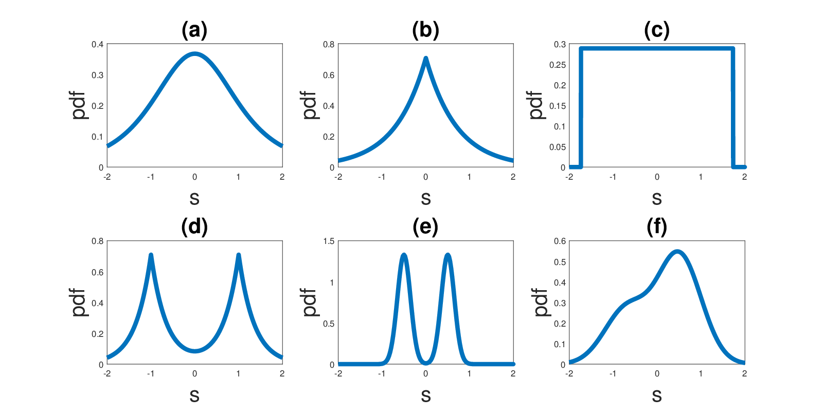
where is the Amari Error defined in (47) and is the true mixing matrix. Denoting and as the mixing matrix estimates of Comon’s ICA algorithm (full data) and the proposed CICA algorithm, respectively, we expect as the Comon algorithm exhibits no compression and makes use of the full cumulant tensor available. As the relative efficiency approaches 1, the sketch estimate becomes more statistically efficient. We perform our efficiency test on independent components of signal length . The signal length does not affect the results as the dependence of drops out of the relative efficiency measure, for example see [25]. For each of the 100 Monte-Carlo simulations, the independent components are randomly sampled [23] from a range of distributions with unique characteristics that are shown in Figure 4. The true mixing matrix was sampled once and fixed throughout. For each sketch size , 100 simulations were executed where the mixing matrix was estimated and the Amari error was calculated. The variance of the Amari errors was compared with the full data counterpart and plotted as the relative efficiency in Figure 5. Figure 5 shows the relative efficiency as the sketch size increases. As increases the relative efficiency approaches 1 (i.e. as statistically efficient as using the full cumulant tensor with no compression). It is evident that there is a trade-off between the rate of compression and the statistical efficiency, for instance, the smaller the sketch size the greater the loss of statistical efficiency. This is to be expected as the harsher you compress the data the more loss of information you experience. Nontheless, the tradeoff is controlled, for example, a sketch of size has a drop of around of efficiency.

6.3 Cylinder Velocity Field
We analyse and compare the proposed CICA scheme on a dataset consisting of a flow field around a cylinder obstruction as depicted in Figure 6. Using ICA, one can obtain a model that describes the fluctuations of the streamwise velocity field around it’s mean value as a function of time. Details of the experimental set up can be seen in [56, 57]. The dataset is of size consisting of 14400 spatial locations over 100 time intervals. Here we compare our proposed CICA scheme with the well-known fast ICA algorithm [58], as well the JADE [52] and Comon algorithm [32] which, like the proposed CICA scheme, are cumulant based.An initial prewhitening stage inferred the prewhiten matrix . Each algorithm then estimated the , resulting in a mixing matrix estimate . For the proposed CICA scheme, the IPG version was used with a SRHT matrix , however ASD version produces similar reconstructions. Figure 7 shows the 8 independent components which describe the fluctuations of the streamwise velocity around the cylinder obtained by Fast ICA, JADE, Comon and CICA, respectively. For our proposed CICA algorithm, a sketch of size is used. Visually comparing the reconstructions, one can see that the CICA algorithm performs competitively with negligible artifacts present. Moreover, the CICA scheme achieves a compression rate of approximately 3 in comparison to the other cumulant based ICA methods discussed.
Next, we compare the effect of the sketch size on the resulting reconstructions. A sketch size of and are considered with the reconstructions shown in Figure 8. For , the sketch is of sufficient size to successfully identify the unique fluctuations of the velocity field, however, due to the harsher compression rate some notable artefacts are present. For example, in the first and third fluctuations there are some oscillating type artifacts which can be attributed to the higher frequencies in the system. Furthermore, the sketch of size fails to identity the main fluctuations of the velocity field.


7 Conclusion
In this paper we initially showed that a low dimensional model set exists for the ICA problem. It was demonstrated theoretically that a RIP exists for the ICA model using Gaussian ensembles provided the sketch size was set proportionally to the model set dimensions, which in turn induced the existence of an instance optimal decoder. The theoretical results were empirically validated by showing the location of a sharp phase transition between a state of unsuccessful inference to a state of successful inference of the ICA mixing matrix as the sketch size increased. Using both synthetic and real data, we analysed the robustness of the proposed CICA algorithms and highlighted the effect of choosing the sketch size . Furthermore, the particular branch of compressive learning was discussed that consists of sketching distribution free models (e.g. PCA, ICA) that leverage some intermediary statistic space, here the space of cumulant tensors, to form the sketch. This poses some interesting open questions on how to design a sketch given other distribution free models and how the low dimension nature of the model set manifests itself structurally, in terms of sparsity, low rank, etc. to construct a practical sketching decoder.
Acknowledgements
This work was supported by the ERC Advanced grant, project C-SENSE (ERC-ADG-2015-694888). Mike E. Davies is also supported by a Royal Society Wolfson Research Merit Award.
Data Availability Statement
The data used in Section 6.3 is available at the repository https://github.com/jonnyhigham/POD_DMD.
Code Availability
A MATLAB implementation of the proposed CICA algorithms are available at the repository https://gitlab.com/mpsheehan1995/CICA.
References
- [1] Rémi Gribonval, Gilles Blanchard, Nicolas Keriven, and Yann Traonmilin. Compressive statistical learning with random feature moments. Mathematical Statistics and Learning, 3(2):113–164, 2021.
- [2] Remi Gribonval, Antoine Chatalic, Nicolas Keriven, Vincent Schellekens, Laurent Jacques, and Philip Schniter. Sketching data sets for large-scale learning: Keeping only what you need. IEEE Signal Processing Magazine, 38(5):12–36, 2021.
- [3] N. Keriven, A. Bourrier, R. Gribonval, and P. Pérez. Sketching for large-scale learning of mixture models. Information and Inference: A Journal of the IMA, 7(3):447–508, 2018.
- [4] A. Hyvärinen and E. Oja. Independent component analysis: algorithms and applications. Neural networks, 13(4-5):411–430, 2000.
- [5] E. Oja, K. Kiviluoto, and S. Malaroiu. Independent component analysis for financial time series. In Proceedings of the IEEE 2000 Adaptive Systems for Signal Processing, Communications, and Control Symposium (Cat. No.00EX373), pages 111–116, 2000.
- [6] R. Vigario, J. Sarela, V. Jousmiki, M. Hamalainen, and E. Oja. Independent component approach to the analysis of eeg and meg recordings. IEEE Transactions on Biomedical Engineering, 47(5):589–593, 2000.
- [7] A. Rahimi and B. Recht. Random features for large-scale kernel machines. In Advances in neural information processing systems, pages 1177–1184, 2008.
- [8] L. P. Hansen. Large sample properties of generalized method of moments estimators. Econometrica, 50(4):1029–1054, 1982.
- [9] Alastair R Hall. Generalized method of moments. A Companion to Theoretical Econometrics, pages 230–255, 2003.
- [10] G. Cormode, M. Garofalakis, P. J. Haas, and C. Jermaine. Synopses for massive data: Samples, histograms, wavelets, sketches. Foundations and Trends in Databases, 4(1–3):1–294, 2012.
- [11] J. A. Tropp, A. Yurtsever, M. Udell, and V. Cevher. Streaming low-rank matrix approximation with an application to scientific simulation. SIAM Journal on Scientific Computing, 41(4):A2430–A2463, 2019.
- [12] S. Guha, A. Meyerson, N. Mishra, R. Motwani, and L. O’Callaghan. Clustering data streams: Theory and practice. IEEE Transactions on Knowledge and Data Engineering, 15(3):515–528, 2003.
- [13] G. Cormodea and S Muthukrishnanb. An improved data stream summary: the count-min sketch and its applications. Journal of Algorithms, 55:58–75, 2005.
- [14] J. A. Tropp, A. Yurtsever, M. Udell, and V. Cevher. Practical sketching algorithms for low-rank matrix approximation. SIAM Journal on Matrix Analysis and Applications, 38(4):1454–1485, 2017.
- [15] S. Har-Peled and S. Mazumdar. On coresets for k-means and k-median clustering. In Proceedings of the thirty-sixth annual ACM symposium on Theory of computing, pages 291–300, 2004.
- [16] D. Feldman, M. Schmidt, and C. Sohler. Turning big data into tiny data: Constant-size coresets for k-means, PCA, and projective clustering. SIAM Journal on Computing, 49(3):601–657, 2020.
- [17] C. Boutsidis, A. Zouzias, and P. Drineas. Random projections for -means clustering. In Advances in Neural Information Processing Systems, pages 298–306, 2010.
- [18] R. Calderbank, S. Jafarpour, and R. Schapire. Compressed learning: Universal sparse dimensionality reduction and learning in the measurement domain. 2009.
- [19] D. L. Donoho. Compressed sensing. IEEE Transactions on Information Theory, 52(4):1289–1306, 2006.
- [20] J. Tang, S. Alelyani, and H. Liu. Feature selection for classification: A review. Data classification: Algorithms and applications, page 37, 2014.
- [21] I. T. Jolliffe and J. Cadima. Principal component analysis: a review and recent developments. Philosophical Transactions of the Royal Society A: Mathematical, Physical and Engineering Sciences, 374(2065):20150202, 2016.
- [22] M. Sela and R. Kimmel. Randomized independent component analysis. In Science of Electrical Engineering (ICSEE), IEEE International Conference on the Science of Electrical Engineering, pages 1–5. IEEE, 2016.
- [23] F.R. Bach and M.I. Jordan. Kernel independent component analysis. Journal of machine learning research, 3(Jul):1–48, 2002.
- [24] K. Muandet, K. Fukumizu, B. Sriperumbudur, B. Schölkopf, et al. Kernel mean embedding of distributions: A review and beyond. Foundations and Trends® in Machine Learning, 10(1-2):1–141, 2017.
- [25] M. P. Sheehan, M. S. Kotzagiannidis, and M. E. Davies. Compressive independent component analysis. In 2019 27th European Signal Processing Conference (EUSIPCO), pages 1–5. IEEE, 2019.
- [26] M. P. Sheehan, A. Gonon, and M. E. Davies. Compressive learning for semi-parametric models. arXiv preprint arXiv:1910.10024, 2019.
- [27] A. J. Bell and T. J. Sejnowski. An information-maximization approach to blind separation and blind deconvolution. Neural Comput., 7(6):1129–1159, November 1995.
- [28] L. De Lathauwer. Signal processing based on multilinear algebra. Katholieke Universiteit Leuven Leuven, 1997.
- [29] P. Comon. Tensor diagonalization, a useful tool in signal processing. IFAC Proceedings Volumes, 27(8):77 – 82, 1994. IFAC Symposium on System Identification (SYSID’94), Copenhagen, Denmark, 4-6 July.
- [30] P. Comon. Tensor decompositions, state of the art and applications. arXiv preprint arXiv:0905.0454, 2009.
- [31] L. De Lathauwer, B. De Moor, and J. Vandewalle. An introduction to independent component analysis. Journal of Chemometrics: A Journal of the Chemometrics Society, 14(3):123–149, 2000.
- [32] P. Comon. Independent component analysis, a new concept? Signal processing, 36(3):287–314, 1994.
- [33] S. Szarek. Nets of grassmann manifold and orthogonal group. In Proceedings of Research Workshop on Banach Space Theory, pages 169–186, 06 1981.
- [34] E. J. Candès and M. B. Wakin. An introduction to compressive sampling. IEEE signal processing magazine, 25(2):21–30, 2008.
- [35] E. J. Candes and Y. Plan. Tight oracle inequalities for low-rank matrix recovery from a minimal number of noisy random measurements. IEEE Transactions on Information Theory, 57(4):2342–2359, 2011.
- [36] A. Bourrier, M. E. Davies, T. Peleg, P. Pérez, and R. Gribonval. Fundamental performance limits for ideal decoders in high-dimensional linear inverse problems. IEEE Transactions on Information Theory, 60(12):7928–7946, 2014.
- [37] T. Blumensath. Sampling and reconstructing signals from a union of linear subspaces. IEEE Trans. Information Theory, 57(7):4660–4671, 2011.
- [38] F. Krahmer and R. Ward. New and improved johnson–lindenstrauss embeddings via the restricted isometry property. SIAM Journal on Mathematical Analysis, 43(3):1269–1281, 2011.
- [39] J. A. Tropp. Improved analysis of the subsampled randomized Hadamard transform. Advances in Adaptive Data Analysis, 3(1):115–126, 2011.
- [40] N. Ailon and B. Chazelle. Approximate nearest neighbors and the fast Johnson-Lindenstrauss transform. In Proceedings of the thirty-eighth annual ACM symposium on Theory of computing, pages 557–563, 2006.
- [41] H. Rauhut, R. Schneider, and Ž. Stojanac. Low rank tensor recovery via iterative hard thresholding. Linear Algebra and its Applications, 523:220–262, 2017.
- [42] G. Puy, M. E. Davies, and R. Gribonval. Recipes for stable linear embeddings from Hilbert spaces to . IEEE Transactions on Information Theory, 63(4):2171–2187, 2017.
- [43] R. Vershynin. Introduction to the non-asymptotic analysis of random matrices. In Compressed Sensing: Theory and Applications, pages 210–268. Cambridge University Press, 2012.
- [44] T. Blumensath and M. E. Davies. Iterative thresholding for sparse approximations. Journal of Fourier analysis and Applications, 14(5-6):629–654, 2008.
- [45] T. Blumensath and M. E. Davies. Iterative hard thresholding for compressed sensing. Applied and computational harmonic analysis, 27(3):265–274, 2009.
- [46] J. F. Cardoso, B. L. R. De Moor, and M. S. Moonen. A tetradic decomposition of 4th-order tensors : Application to the source separation problem. pages 375–382, Amsterdam, 1995. Elsevier;.
- [47] J. F. Cardoso. Fourth-order cumulant structure forcing: application to blind array processing. In [1992] IEEE Sixth SP Workshop on Statistical Signal and Array Processing, pages 136–139, 1992.
- [48] J. Cadzow. Signal enhancement-a composite property mapping algorithm. IEEE Trans. Acoust. Speech Signal Process., 36:49–62, 1988.
- [49] Z. Wen and W. Yin. A feasible method for optimization with orthogonality constraints. Math. Program., 142(1–2):397–434, December 2013.
- [50] J. Crank and P. Nicolson. A practical method for numerical evaluation of solutions of partial differential equations of the heat-conduction type. In Mathematical Proceedings of the Cambridge Philosophical Society, volume 43, pages 50–67. Cambridge University Press, 1947.
- [51] F. Woolfe, E. Liberty, V. Rokhlin, and M. Tygert. A fast randomized algorithm for the approximation of matrices. Applied and Computational Harmonic Analysis, 25(3):335 – 366, 2008.
- [52] J. F. Cardoso and A. Souloumiac. Blind beamforming for non-gaussian signals. In IEE proceedings F (radar and signal processing), volume 140, pages 362–370. IET, 1993.
- [53] D. Amelunxen, M. Lotz, M. B. McCoy, and J. A. Tropp. Living on the edge: phase transitions in convex programs with random data. Information and Inference: A Journal of the IMA, 3(3):224–294, 2014.
- [54] S. Amari, A. Cichocki, and H. Yang. A new learning algorithm for blind signal separation. In Advances in neural information processing systems, pages 757–763, 1996.
- [55] R. A. Fisher. On the mathematical foundations of theoretical statistics. Philosophical Transactions of the Royal Society of London. Series A, Containing Papers of a Mathematical or Physical Character, 222:309–368, 1922.
- [56] J.E. Higham, W. Brevis, and C.J. Keylock. Implications of the selection of a particular modal decomposition technique for the analysis of shallow flows. Journal of Hydraulic Research, 56(6):796–805, 2018.
- [57] Wernher Brevis and Manuel García-Villalba. Shallow-flow visualization analysis by proper orthogonal decomposition. Journal of Hydraulic Research, 49(5):586–594, 2011.
- [58] A. Hyvarinen. Fast and robust fixed-point algorithms for independent component analysis. IEEE Transactions on Neural Networks, 10(3):626–634, 1999.
- [59] Kenneth L Clarkson. Tighter bounds for random projections of manifolds. In Proceedings of the twenty-fourth annual symposium on Computational geometry, pages 39–48, 2008.
- [60] Brett W. B. Tamara G. K. Tensor Decompositions and applications. 51(3):455–500, 2009.
- [61] Rodney Coleman. Calculus on Normed Vector Spaces. Springer New York, 2012.
- [62] A. Rahimi and B. Recht. Weighted sums of random kitchen sinks: Replacing minimization with randomization in learning. In Advances in neural information processing systems, pages 1313–1320, 2009.
Appendix A Proof of Lemma 4.1
To prove Lemma 4.1, we use a similar line of argument to Clarkson in [59] by splitting the normalized secant set into the set of short and long secants parametrized by a distance . First we state an important lemma on covering the model set intersected with the unit sphere in , where , denoted by (e.g. ), that will used later in the proof.
Lemma A.1 (Covering number of ).
The covering number of with respect to the Frobenius norm is
| (49) |
Proof.
Recall that has the decomposition such that where and . As the Frobenius norm is rotationally invariant then the following holds for all . Our argument constructs an -net for by covering the sets and respectively. As , it is sufficient to consider . Then we take to be an - net for . As is a dimensional subspace, then
Next, we cover the set of orthogonal matrices denoted . We follow a similar argument to [41, 35] by letting , where
is the maximum column norm of a matrix . It is straightforward to see that since the columns of an orthogonal matrix are unit normed. It can be seen in [35] that an -net , denoted by , has a covering number
Now let , and remark that
It remains to show that for all there exists such that .
Fix and note the decomposition . Then there exists with and obeying and . This gives
The first part of the last line gives
From line 1 to 2, the identity on pages [477-478] of [60] was used. From line 2 to 3 we have used the Cauchy-Schwarz inequality, from line 3 to 4 we have used the equality and from line 4 to 5 we have used the identity in [41]. Finally, notice that as is orthogonal
Therefore
∎
Continuing, we let define the product set between the set of orthogonal matrices and the set of super symmetric cumulant tensors defined in (16) and define the map by
| (50) |
for all . Let be the tensor corresponding to the image of the map . It is insightful to decompose the normalised secant set into the set of long and short secants parametrised by some distance [59]. The set of long secants of is defined as
| (51) |
Furthermore, the set of short secants is the complement to the set of long secants defined by
| (52) |
Remark 1.
As the model set is conic (see supplementary material), it is sufficient to cover the normalised secant set of , where denotes the unit Frobenius ball centred at 0, since we have .
As a result we can decompose the normalised secant set as follows
| (53) | ||||
We begin by covering the set of long secants .
Lemma A.2 (Long Secants Covering Number).
Let be an -cover for . Then is an -cover for with associated covering number of
| (54) |
Proof.
Continuing, we cover the set of short secants. We begin by stating some preliminary lemmas.
Lemma A.3 (Taylor Approximation Error).
Let be defined as in (50) and let define the first order differential of evaluated at the point . Further assume that . Then , , we have
| (55) |
where
Proof.
w.l.o.g consider the vectorized function such that
Using Taylor’s theorem [61, p. 110] of evaluated at the point , we get
| (56) | ||||
where and denote the Jacobian and Hessian of evaluated at and , for , denotes a point on the line segment between and . For shorthand let , and denote the integer , we then have
where . w.l.o.g let , we have that
-
It can be seen that (see supplementary material)
(57) where
and the matrix , where is the th unit basis vector. Using the properties of the Kronecker product and the triangle inequality we get
Assuming that the diagonal tensor has bounded support , then it follows that
(58) -
It can be seen that (see supplementary material)
(59) where and
Similarly to , we get
-
It can be easily shown that
(60) therefore
(61)
It therefore follows that
| (62) |
and,
| (63) |
∎
Lemma A.4 (Bounded Curvature).
Let be defined as in (50) and let define the first order differential of evaluated at the point . Further assume that . Then , , we have
| (64) |
where
Proof.
Lemma A.5 (Bounded Gradient).
Proof.
As in A.3, we consider the vectorized function w.l.o.g. It can be seen that the 1st order differential (see supplementary material) has the following decomposition
| (68) |
where
| (69) |
Furthermore, the partial derivative with respect to the super symmetric cumulant tensor is defined as
where . Equivalently, (67) can be rewritten as
| (70) |
where . We therefore have
As is equivariant in , we can set w.l.o.g. As a result and reduces to
For shorthand, let and noting that , we have
As a result, we have that
It can be easily shown that for
and for
We therefore have
Now assume that for all , therefore
In the last line, we assume w.l.o.g that . We have therefore proved that
| (71) |
yielding . ∎
We have the following lemma to cover the set of short secants.
Lemma A.6 (Short Secants Covering Number).
Let be an - cover for and considering the following:
- 1.
(Taylor approximation Lemma A.3)
- 2.
(bounded curvature Lemma A.4)
- 3.
(bounded gradient Lemma A.5),
where is defined in Eqn. 50 and defines the first order differential of evaluated at the point . Then given , and , where and , we have
| (72) |
where .
Proof.
Given that , we have that and . Therefore
Now dividing by gives:
In the last line, we have used the fact that bounded (inverse) gradient implies Lipschitzness. ∎
As a result, the set of bounded tangent vectors, defined by
forms a generalized -cover for with covering number (see Lemma 4.3 of [59])
From (53), we can bound the covering number of the normalized secant set:
Note that by definition , therefore . As a result
Appendix B Proof of Theorem 4.2
Proof.
Let denote the expected cumulant tensor and the cumulant tensor computed from the finite data samples as in (33). Note that the feature function in (32) can be equivalently written as . Using the RIP result from Theorem 4.1 and by assuming the independent components have bounded support , we have
where the norm is invariant under the orthogonal transformation . Next we apply the concentration of averages lemma (lemma 4) of [62] to get with probability on the drawing of both and that
∎