Minimizing entropy for translation surfacesThanks: The authors would like to thank L.Bétermin for suggesting the connection with his work [2] and Samuel Lelièvre for helpful comments. We are also grateful to the referee for their helpful comments and suggestions. The second author was supported by ERC Grant 833802-Resonances and EPSRC grant EP/T001674/1.

We begin by recalling for the purposes of motivation a well known classical result of Katok from 1982 for compact negatively curved surfaces. Let $\mathcal{M}_{g}$ denote the space of negatively curved $C^{\infty}$ Riemannian metrics of unit volume on a compact orientable surface of genus $g\geqslant 2$. The entropy function $h:\mathcal{M}_{g}\to\mathbb{R}^{+}$ can be defined in terms of the growth rate of closed geodesics

where $\rho\in\mathcal{M}_{g}$ and $\ell_{\rho}(\gamma)$ denotes the length of a closed $\rho$-geodesic $\gamma$. When restricted to metrics of unit volume the entropy is minimized precisely at metrics of constant curvature [10].

In this note we want to formulate a partial analogue of this result for translation surfaces. Informally, a translation surface can be thought of as a closed surface obtained from taking a collection of polygons in the plane and gluing together parallel edges via isometries (see [19] for a good introduction to translation surfaces). A translation surface has a finite number of singularities with cone angles of the form $2\pi(k+1)$ where $k\in\mathbb{N}$. To see what this means, consider the following construction: let $k\in\mathbb{N}$ and take $(k+1)$ copies of the upper half-plane with the usual metric and $(k+1)$ copies of the lower half-plane. Then glue them together along the half infinite rays $[0,\infty)$ and $(-\infty,0]$ in cyclic order (Figure 1).

There are a few equivalent definitions of translation surfaces that appear in the literature. We will use the following definition (see [18]).

Dankwart associated to a translation surface $X$ with a non-empty finite singularity set $\Sigma$ an analogous notion of entropy [6]. Given $k_{1},\ldots,k_{n}\geqslant 1$ we can denote by $\mathcal{H}^{1}(k_{1},\ldots,k_{n})$ the space of unit area translation surfaces with $n$ singularities in $\Sigma$ with cone angles $2\pi(k_{1}+1),\ldots,2\pi(k_{n}+1)$. The entropy function $h:\mathcal{H}^{1}(k_{1},\ldots,k_{n})\to\mathbb{R}^{+}$ can be defined in terms of the growth rate of closed geodesics containing a singular point

where $\ell_{X}(\gamma)$ denotes the length of a closed geodesic $\gamma$ on $X$ which includes a singular point from $\Sigma$.¹¹ 1 This avoids the complication of accounting for cylinders of uncountably many parallel geodesics. Alternatively, we could account for these by counting only their free homotopy classes, but then their polynomial growth does not affect the definition of the entropy. The entropy is continuous and bounded below, and can become arbitrarily large (when a closed geodesic becomes sufficiently small) even when the total area is normalized (although it will always be finite) [6]. We restrict the type of translation surfaces we will consider as follows:

1. (1)

   Firstly, we fix a unit area square tiled surface $X_{0}$, which is a union of squares where the singularities occur at the vertices and the singularities have a common cone angle; and

2. (2)

   Secondly, we consider the three dimensional orbit $SL(2,\mathbb{R})X_{0}$ associated to the linear action of the group $SL(2,\mathbb{R})$ [18].

The surfaces described in (1) are known as square tiled surfaces (see [13] for a good introduction to square tiled surfaces).

Note that the area of surfaces in the orbit $SL(2,\mathbb{R})X_{0}$ coincide with the area of $X_{0}$.

Our main result is the following theorem.

We take the convention that we identify surfaces that are identical up to a rotation (i.e., the action of $SO(2)$).

Theorem 1.2 applies to the following simple example and to the examples listed in §3. Furthermore, it is known that every stratum contains an equilateral translation surface [4].

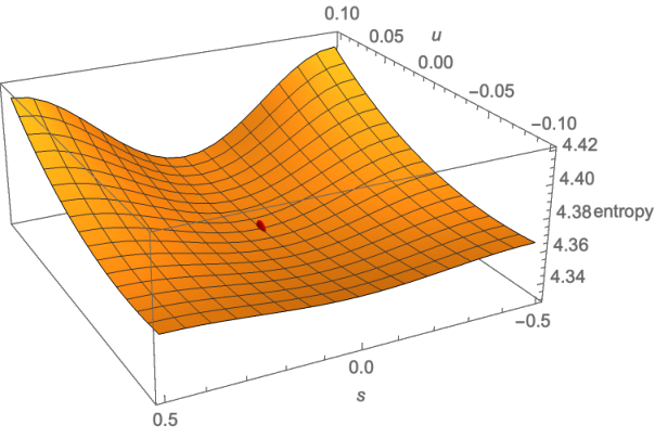
In Figure 2 we have plotted an approximation²² 2 This plot was obtained using the method for approximating the entropy of surfaces in the orbit of $X_{0}$ derived in Section 8. to the entropy of the surfaces.

and indicated the point above $X_{1}=X_{2}$. We confirm empirically that the entropy is locally minimized at $X_{1}=X_{2}$. A simple symmetry argument confirms that $X_{0}$ is also a critical point.

If we homothetically scale any translation surface by a factor $c>0$ then the entropy scales by $1/c$, but the area scales by $c^{2}$. Therefore, it is appropriate to consider translation surfaces scaled to have unit area, say. Let $\mathcal{H}^{1}[k,n]$ denote a stratum of unit area surfaces with $n$ singularities, each with the same cone angle $2\pi(k+1)$, where $n,k\geqslant 1$. In light of Theorem 1.2 we conjecture³³ 3 This conjecture may be related to the “Universal Optimality Conjecture” (see Conjecture 9.4 in Section 9 of [5]). the following:

In Sections 2 and 3 we present some preliminary results on entropy. In Section 4 we will present some more examples of surfaces satisfying the hypotheses in (1). In Sections 5 and 6 we introduce the main technical ingredients in the proof: Montgomery’s and Bernstein’s Theorems, respectively. In Section 7 we complete the proof of Theorem 1.2. In Section 8 we derive a method for approximating the entropy of the types of surfaces we consider in this note. In the final section we collect together some final comments and questions.

Fix a translation surface $X$ with singularity set $\Sigma$. A saddle connection $s$ is a straight line on $X$ between two singularities (which does not contain a singularity in its interior).

The entropy can be defined in terms of the growth of saddle connection paths, which are geodesics joining singularities. Let $i(s)$ and $t(s)$ denote the initial and terminal singularity, respectively, of an oriented saddle connection $s$. Given a translation surface $X$, let $\underline{s}=s_{1}\ldots s_{n}$ denote an oriented saddle connection path of length $\ell(\underline{s})$ where consecutive oriented saddle connections $s_{i}$ and $s_{i+1}$ form a locally distance minimizing geodesic. In particular, the angle between $s_{i}$ and $s_{i+1}$, for $1\leqslant i\leqslant n-1$, should be greater than or equal to $\pi$ on both sides. We write $\ell(\underline{s})=\sum_{i=1}^{n}\ell(s_{i})$ where $\ell(s_{i})$ denotes the length of $s_{i}$. The following definition is easily seen to be equivalent to the definition from the introduction.

Whenever $\Sigma\neq\emptyset$ we have that $h(X)>0$.

There is a useful alternative formulation which we now present in the next lemma that follows from Definition 2.1 (see [11]).

We conclude this section by introducing a notational device for certain sequences of saddle connections that will be used in the proof of Lemma 3.2 in the next section.

Let $\underline{s}=s_{1}\dots s_{n}$ be a saddle connection path. Consecutive saddle connections in $\underline{s}$ will join at an angle allowed by the condition that $\underline{s}$ is a geodesic, and so typically it will not be a singular connection. However, exceptionally $\underline{s}$ may have substrings of saddle connections that form singular connections. Assuming that we only consider singular connections $e$ that are maximal with respect to $\underline{s}$ (i.e. there does not exist another substring $e^{\prime}$ of $\underline{s}$ such that $e$ is a substring of $e^{\prime}$ and $e^{\prime}$ is also a singular connection), then $\underline{s}$ has a unique decomposition of the form $\underline{s}=e_{1}\ldots e_{m}$, where the $e_{i}$ are singular connections, and for $1\leqslant i<m$, $e_{i}e_{i+1}$ is not a singular connection (i.e., the clockwise angle between them is greater than $\pi$).

Fix $X_{0}\in\mathcal{H}^{1}[k,n]$, a unit area square tiled surface with $n$ singularities with cone angle $2\pi(k+1)$ satisfying the conditions in (1) in the introduction. Note that $X_{0}$ will be tiled by $n(k+1)$ squares.

In order to study surfaces $AX_{0}$, where $A\in SL(2,\mathbb{R})$, we can denote by

the scaled standard lattice (minus the origin) and $A(\Lambda)=\{\left(A\left(\begin{smallmatrix}p\\ q\end{smallmatrix}\right)\right)^{T}\hbox{ : }(p,q)\in\Lambda\}$ its image under the linear action of $A$. We can then associate functions $f_{t}:SL(2,\mathbb{R})\to\mathbb{R}^{+}$ for each $t>0$ by

where $\|\underline{v}\|$ is the usual Euclidean length of $\underline{v}\in\mathbb{R}^{2}$.

We will relate the entropy $h(AX_{0})$ of $AX_{0}$ to $f_{t}(A)$ by taking advantage of the additional structure of the set of saddle connection paths on $AX_{0}$.

The functions $f_{t}(\cdot)$ have the following useful properties.

Lemma 3.2 gives a particularly useful characterization of the entropy. As a first application we have the following.

We are interested in square tiled surfaces where the vertex of each square is a singularity with a common cone angle. We note that any square tiled surface consisting of $N$ square tiles can be represented by a pair of permutations $(h,v)\in Sym(N)\times Sym(N)$, where $h,v$ represent the gluings of the horizontal and vertical edges of the squares, respectively (see [16]). We recall that for translation surfaces $X\in\mathcal{H}^{1}(k_{1},\ldots,k_{n})$ the genus $g$ satisfies $2g-2=\sum_{i=1}^{n}k_{i}$ [18]. We can consider a few simple examples.

We can next consider two different types of stair examples.

Finally, we can consider a well known example of Forni [7] and Herrlich-Schmithüsen [8].

In order to analyze $f_{t}(\cdot)$, and thus use Lemma 3.2 to study the entropy, it is convenient to first study a related function $F_{t}(L)$, where $L$ is a unimodular lattice, i.e., of the form $A(\Lambda)$ for some $A\in SL(2,\mathbb{R})$. Throughout we consider the lattices up to rotation. In particular, this will allow us to use a result of Montgomery.

We see that $F_{t}(L)$ is finite provided $t>0$. Moreover, on this domain the function $F_{t}(L)$ has a smooth dependence on $t$ and $L$. The next result describes lattices which minimize $F_{t}(L)$ [15] (see also [1], Appendix A). Let $L_{\Delta}$ denote the equilateral triangular lattice.

To proceed we need to relate $F_{t}(\cdot)$ and $f_{t}(\cdot)$. This requires a result of Bernstein on completely monotone functions.

We will be particularly interested in the following example.

The interest in completely monotone functions is that they are the Laplace transform of positive functions, as is shown in the following classical theorem [3].

An account appears, for example, in the book of Widder (see Chapter IV, §12 [17]).

We want to use use Proposition 6.3 to convert Proposition 5.2 for $F_{t}(\cdot)$ into the corresponding result for $f_{t}(\cdot)$, in Proposition 7.1 below.

For completeness we recall the elegant short proof of Bétermin.

We can now complete the proof of Theorem 1.2.

Let $A\in SL(2,\mathbb{R})$ be chosen so that $AX_{0}$ has a triangulation by equilateral triangles and let $B\in SL(2,\mathbb{R})$ be an element in the group which does not correspond to triangulation by equilateral triangles.

We can use the functions $f_{t}(A)$ and $f_{t}(B)$ to compare the entropies $h(A)$ and $h(B)$ of $AX_{0}$ and $BX_{0}$, respectively. By Proposition 7.1 we know that that $f_{t}(A)<f_{t}(B)$ for all $t>0$. By part 2 of Lemma 3.2 the entropy $h(A)$ for the surface $AX_{0}$ is the unique value such that $f_{h(A)}(A)=\frac{1}{k}$. However, by part 1 of Lemma 3.2 the function $t\mapsto f_{t}(B)$ is monotone decreasing so the solution $f_{h(B)}(B)=\frac{1}{k}$ implies that $h(B)>h(A)$.

Let $X_{0}$ denote a square tiled surface in $\mathcal{H}^{1}[k,n]$. In this section we present a method for finding arbitrarily good approximations to $h(A)$, for a given $A\in SL(2,\mathbb{R})$, and calculate the error terms of these approximations. We will then use this method to approximate $h(\Delta)$, the entropy of the equilateral surface in Example 1.3.

Let $N\in\mathbb{N}$ and define $\mathbb{Z}_{N}=\{n\in\mathbb{Z}:|n|\leqslant N\}$. We define the finite square lattice

Note that the first few derivatives of $f_{t}^{(N)}(A)$ also give approximations to the respective derivatives of $f_{t}(A)$. Finally, we note that the region

has area $\hbox{\rm Area}(P(A))=\frac{1}{n(k+1)}$ and its translates by $A\left(\frac{1}{\sqrt{n(k+1)}}\mathbb{Z}^{2}\right)$ tile the plane $\mathbb{R}^{2}$.

The following simple lemma allows us to bound the error in the approximations.

We will now use the $f_{t}^{N}(A)$ and the above lemma to approximate $h(\Delta)$, where $h(\Delta)$ denotes the entropy of the equilateral surface in Example 1.3 (the unique equilateral surface in $\mathcal{H}^{1}[2,1]$.

It follows from Lemma 3.2 that $h(\Delta)$ is the unique $t>0$ such that $f_{t}(\Delta)=1/2$.

References

- [1] L. Bétermin, Lattices energies and variational calculus, Ph.D. thesis, Université Paris-Est. (https://tel.archives-ouvertes.fr/tel-01227814/document).
- [2] L. Bétermin, Two dimensional theta functions and crystallization among Bravais lattices, Siam J. Math. Anal., 48 (2016) 3236–3269 .
- [3] S. N. Bernstein, Sur les fonctions absolument monotones, Acta Mathematica. 52 (1929) 1–66.
- [4] C. Boissy and S. Geninska, Systoles in translation surfaces, Bull. Soc. Math. France, 2 (2021) 417-438.
- [5] H. Cohn and A. Kumar, Universally optimal distribution of points on spheres, J. Amer. Math. Soc., 20 (2007) 99–148.
- [6] K. Dankwart, PhD thesis, Bonn, On the large-scale geometry of flat surfaces, 2014. (https://bib.math.uni-bonn.de/downloads/bms/BMS-401.pdf).
- [7] G. Forni, On the Lyapunov exponents of the Kontsevich–Zorich cocycle, Handbook of Dynamical Systems v. 1B, B. Hasselblatt and A. Katok, eds., Elsevier, (2006), 549–580.
- [8] F. Herrlich and G. Schmithüsen, An extraordinary origami curve, Mathematische Nachrichten 281, No. 2, (2008) 219 – 237.
- [9] A. Katok, G. Knieper, M. Pollicott, H. Weiss, Differentiability and analyticity of topological entropy for Anosov and geodesic flows, Inventiones Mathematicae, 98 (1989) 581–597.
- [10] A. Katok, Entropy and closed geodesies, Ergodic Theory and Dynamical Systems, 2 (1982) 339–365.
- [11] W. Kim and S. Lim, Notes on the values of volume entropy of graphs, Discrete and Continuous Dynamical Systems. Series A, 9 (2020) 5117–5129.
- [12] S. Lim, Minimal volume entropy for graphs, Transactions of the American Mathematical Society, 360 (2008), 5089–5100.
- [13] C. Matheus, Three lectures on square-tiled surfaces, 2018. (https://if-summer2018.sciencesconf.org/data/pages/origamis_Grenoble_matheus_3.pdf).
- [14] K. Miller and S. Samko, Completely monotonic functions. Integral Transform. Spec. Funct. 12 (2001) 389–402.
- [15] H. Montgomery, Minimal theta functions, Glasgow Mathematical Journal, 30 (1988) 75 – 85.
- [16] G. Schmithüsen, Veech groups of origamis, PhD Thesis, Karlsruhe, 2005. (https://www.math.kit.edu/iag3/˜schmithuesen/media/dr.pdf)
- [17] D. Widder, Laplace transform, Dover, New York, 2010.
- [18] A. Wright, Translation surfaces and their orbit closures: an introduction for a broad audience, EMS Surv. Math. Sci. 2 (2015), no. 1, 63–108.
- [19] A. Zorich, Flat surfaces, Frontiers in number theory, physics, and geometry I (2006), 437–583.