Adversarial Attack across Datasets
Abstract
Existing transfer attack methods commonly assume that the attacker knows the training set (e.g., the label set, the input size) of the black-box victim models, which is usually unrealistic because in some cases the attacker cannot know this information. In this paper, we define a Generalized Transferable Attack (GTA) problem where the attacker doesn’t know this information and is acquired to attack any randomly encountered images that may come from unknown datasets. To solve the GTA problem, we propose a novel Image Classification Eraser (ICE) that trains a particular attacker to erase classification information of any images from arbitrary datasets. Experiments on several datasets demonstrate that ICE greatly outperforms existing transfer attacks on GTA, and show that ICE uses similar texture-like noises to perturb different images from different datasets. Moreover, fast fourier transformation analysis indicates that the main components in each ICE noise are three sine waves for the R, G, and B image channels. Inspired by this interesting finding, we then design a novel Sine Attack (SA) method to optimize the three sine waves. Experiments show that SA performs comparably to ICE, indicating that the three sine waves are effective and enough to break DNNs under the GTA setting.
1 Introduction
The fast development of Deep neural networks (DNNs) has promoted many artificial intelligence fields ranging from image classificationhe2016deep to natural language translationzhang2019bridging and self-driving carsprakash2021multi. However, lots of studies szegedy2014intriguing; goodfellow2014explaining; carlini2017towards; lin2020nesterov demonstrated that by adding human imperceptible adversarial perturbations to clean input data, even well-trained DNNs can be fooled with high probabilities. This phenomenon indicates that DNNs are vulnerable to adversarial attacks and reveals their robustness issue.
To evaluate the robustness of trained DNNs, lots of adversarial attack generation methods were proposed in recent years. According to how many victim model information the attacker can access, existing adversarial attack methods can mainly be categorized into the following three main stream settings: white-box goodfellow2014explaining; moosavi2016deepfool, query-based black-box brendel2018decision-based; ilyas2018black; cheng2018query, and query-free black-box attack liu2016delving; papernot2017practical, which can be summarized in Table 1. In the white-box attack setting, the attacker can access all information of the victim model to generate adversarial attacks, which is often idealistic and impractical. Query-based black-box attack assumes that except for querying the output or prediction of the victim model, all the other information of the victim model is hidden from the attacker. Among the three settings, query-free black-box attack is the most challenging one because as Table 1 shows, even querying the victim model is also forbidden to the attacker.
| Attack Setting | Information of the target model that can be accessed | ||
|---|---|---|---|
| White-Box |
| ||
| Query-based Black-Box |
| ||
| Query-free Black-Box | Limited information (input-resolution, label-set) | ||
| Generalized Transferable Attack | Non information (/) |

Unfortunately, the victim model is still vulnerable due to the demonstrated transferability of adversarial examples wu2018understanding; wu2020boosting; naseer2019cross-domain; demontis2019why. The transferability-based adversarial attack methods (shorten as transfer attack in the rest of the paper) usually leverage one or a few surrogate white-box models to construct adversarial examples and transfer the obtained adversarial examples to attack the victim model without querying. Though previous works have demonstrated the effectiveness of transfer attacks papernot2017practical; guo2020backpropagating and methods have been developed to improve the transferability of adversarial examples li2020learning; wang2021enhancing, they usually implicitly assume that surrogate white-box models and the victim model are trained on the same dataset or are using the same label set, and their experimental results commonly depend on this assumption. This means the attacker actually knows some information (e.g., input resolution and label set) of the victim model under the query-free black-box attack setting. For example, when the victim model and the victim images are from Cifar-10 krizhevsky2009learning, they assume that the surrogate models are also trained on Cifar-10 rather than ImageNet deng2009imagenet. Despite the three main-stream attack settings, the authors of naseer2019cross-domain proposed a more challenging cross-domain attack setting where the surrogate models and the victim model are trained on different datasets, but they still implicitly assumed that the image resolutions of victim models and the victim model are consistent.
In practice, however, the victim image (and victim model) can randomly come from any dataset with arbitrary label and resolution, and the attacker won’t know which dataset is being used in advance. It is also impractical to retrain new surrogate models for each new dataset. Therefore, we need to assume the surrogate models and the victim model are trained on different datasets with different label sets and different image resolutions. We denote this more practical setting as generalized transferable attack (GTA) because the attacker needs to be generalized to attack images from unknown datasets and attack any unknown models predicting these images. Table 1 illustrates the difference between GTA and the previous attack settings.
In this paper, we aim to investigate the robustness of DNNs under the GTA setting, and explore what kind of attacks can break DNNs under this setting. Although most of the existing transfer attacks are not designed for attacking across datasets, with some careful modifications on the attack loss and rescaling techniques, it is possible to extend existing attacks dong2019evading; xie2019improving; dong2018boosting to this new setting (we will discuss these modifications in Sections 6.1.1 and Appendix). Unfortunately, as will be seen in the experimental results, even with these modifications the existing transfer attacks suffer from poor attack success rates due to the mis-match of label set and input size between source and target models. To tackle these challenges, we sequentially propose two novel methods where the second one is highly inspired by the phenomenons exhibited by the first one.
The first method is inspired by meta-learningfinn2017model; qin2020layer; SNAIL. It uses resources (i.e., some source datasets containing various label sets and input sizes, some white-box models trained on these source data) to meta-train finn2017model; SNAIL; meta-teacher; liu2019metapruning a universal surrogate model for the objective that classification information of each image from any category with any resolution can be erased by attacking the universal surrogate model. After meta-training the universal surrogate model, we use it to erase classification information of new images that are outside the label space and image resolution space of the source datasets. We call the first method Image Classification Eraser (ICE) and will describe the detail in Section 4.
The experimental results in Section 6 will demonstrate the effectiveness of the proposed ICE under the GTA setting. Despite the performance, here we want to emphasize an interesting observation shown by ICE. To save space, we only visualize a few ICE noise examples in Fig.1 and will visualize the noises generated by the other methods in Section 7. Fig. 1 clearly shows that ICE uses similar texture-like noise to perturb different images, even when the images are sampled from different datasets with different resolutions. Moreover, Section 6.5 will demonstrate that the ICE noise generated for each image can be directly used to attack other images from the same or different datasets. In other words, ICE can be viewed as a universal noise generator. Compared with existing universal adversarial attacksmoosavi2017universal; zhang2021data who commonly focus on constructing the adversarial noise that is universal only within a single dataset, ICE is more generalizable because the generated ICE noise is universal not only within a single dataset but also across datasets and resolutions.
As Fig.1 shows, we also analyze noises generated by ICE via fast fourier transformation (FFT) and find that the main components in each ICE noise are three sine waves for the input R, G, and B channels. Each sine wave is represented by the pair of the brightest points in each spectrum diagram. Inspired by this interesting insight, we design the second method Sine Attack (SA) which directly optimizes the three sine waves for the R, G, and B channels. Fig.2 shows the optimized sine signals when we using Cifar-10, Cifar-100, and TieredV56 as source datasets. The experiments in Section 6 demonstrate that SA performs comparably to ICE under the GTA setting, indicating that three particular sine signals are effective adversarial signals under the GTA setting.

The main contributions of our paper are as follows.
- •
To the best of our knowledge, we are the first to propose the challenging and practical generalized transfer attack (GTA) setting. Under GTA, the attacker is acquired to directly attack any images without knowing the image label, the dataset that the image belongs to, and the image resolution, in advance.
- •
To generate adversarial example under the GTA setting, we propose a novel meta-learning inspired method ICE. Throughout experiments in Section 6 demonstrate the effectiveness of the proposed ICE.
- •
Despite the excellent performance of ICE, we also analyze the noises generated by ICE via both experiments and FFT, and we find that ICE can be viewed as a generator for three universal sine signals for the GTA setting. Our finding may inspire researchers to analyze and improve the robustness of DNNs.
- •
Inspired by our finding, we propose another method SA to address the challenging GTA setting. Throughout experiments in Section 6 demonstrate that SA performs comparably to ICE under the GTA setting.
- •
Furthermore, the experiments in Sections 6.5 6.6, 6.7, and 6.9 demonstrate that the ICE noise and SA noise are universal perturbations across images, datasets, resolutions, and tasks. For example, Section 6.9 shows that the SA noise constructed by three sine waves can be directly used to effectively attack object detection models.
2 Background
2.1 Adversarial attack settings
Existing adversarial attack methods ganeshan2019fda; croce2020minimally; wu2020stronger; li2020practical; kaidi2019structured; maksym2020square; xiao2021graph; zhang2021data can mainly be categorized into white-box, query-based black-box, and query-free black-box attacks. Among the three kinds of attacks, white-box attack kurakin2016adversarial is the most effective one because all information of the target model can be leveraged to generate adversarial examples. Query-based black-box attack assumes that some information of the target model is hidden from users and the users can only query the target model and access the hard-label or soft-label predictions. Researchers have proposed many query-based black-box attack methods chen2017zoo; cheng2020signopt; huang2020black; gao2020patch and have shown that adversarial examples can still be effectively generated only based on predictions. The most recently developed query-based methods mainly focus on improving the querying efficiency and reducing the query counts cheng2019improving; li2020qeba; du2020query-efficient; wang2020spanning; yuan2021meta. The query-free black-box attack further assumes that the target model’s prediction is also hidden from users. In this challenging situation, researchers usually generate adversarial examples via attacking surrogate models dong2019evading; xie2019improving. Then, by leveraging the transferability of adversarial examples papernot2016transferability; tramer2017ensemble; nathan2020perturbing, we can directly use the adversarial examples to attack the target model without querying huang2019enhancing; zhou2018transferable; Lu_2020_CVPR. The level of information that the attacker can leverage reduces from white-box to query-free black-box attacks. However, the three most popularly used attack settings still need to know some information of the victim model, which is summarized in Table 1. For example, transfer-based attacks commonly assume the surrogate model and victim model are trained on the same dataset, which indicates that the attacker implicitly knows the dataset, input size, and label set of the victim model.
Beyond the three main stream settings, a few other attack settings have also been studied in recent works li2020practical; nathan2020perturbing; inkawhich2021can; zhang2021data; naseer2019cross-domain. For instance, in no-box attack li2020practical, the attacker can access neither a large scale training data nor pre-trained models on it. To attack a victim image, the no-box attacker needs firstly to collect a mini-training set that contains a small number of images and secondly to train a substitute model for generating adversarial noise on the victim image. Due to the two steps in attacking each victim image, no-box attack is costly to attack a large amount of diverse images in practice. The authors of inkawhich2021can studied the problem where the white-box model and victim model share no label. They firstly query the victim model by using the white-box dataset and obtain the mapping between white-box labels and black-box labels, and then use the white-box models and the resulting mapping to attack victim images. Though their study is interesting, their method is sometimes unrealistic since before attacking, they have to build the mapping via extensively querying the victim model. Universal adversarial perturbation (UAP) zhang2021data aims to obtain a universal perturbation pattern within an image distribution so that adding the perturbation pattern to any clean image sampled from the distribution can possibly produce an adversarial example. However, as will be demonstrated in our experiment, UAP performs not well enough to attack the images sampled from unknown distributions (datasets). The authors of naseer2019cross-domain proposed a cross-domain attack setting where the surrogate models and the victim model are trained on different datasets. However, they also implicitly assumed that the resolutions of victim models and the victim model are consistent, which is still unrealistic in some challenging cases. In this paper, we consider a novel and more challenging problem called generalized transferable attack (GTA) and will detail the GTA setting in Section 3.
2.2 Adversarial perturbation’s frequency characteristic
Some works geirhos2019imagenet-trained; ilyas2019adversarial; das2018shield tried to explain why adversarial perturbation exists from the perspective of frequency. It is demonstrated that DNNs’ predictions are simultaneously determined by image’s low-frequency and high-frequency (including human imperceptible) information, especially the high-frequencyyin2019fourier. For example, by using synthesized texture-shape cue conflict images, the work geirhos2019imagenet-trained demonstrated that ImageNet CNN models are usually more sensitive to image’s texture information than to shape information. Texture is high-frequency information while shape is low-frequency. Via experiments and analysis, the work yin2019fourier demonstrated that instance dependent adversarial perturbations are high frequency signals and used Auto-AugmentationCubuk_2019_CVPR to improve DNNs’ robustness towards high frequency perturbations. Similar high-frequency characteristic was also found in universal adversarial perturbations by zhang2021universal. Since DNNs commonly are sensitive to high-frequency information, their predictions will possibly be determined by adversarial perturbation containing rich high-frequency information rather than the original clean image. Though these previous works have demonstrated the high-frequency characteristic of adversarial perturbation, they didn’t analyze how high the frequency should be, especially under the challenging GTA setting. In this work, inspired by the observation shown in Fig.1, we propose a novel Sine Attack method which directly optimizes the parameters determining not only the frequency but also the sine wave direction and initial phase, for generating effective adversarial attacks under the GTA setting.
3 Generalized transferable attack
GTA can be described as the following attack scene. We have the resources of: 1) source image classification datasets denoted as , , …, . Different datasets have different label sets, with potentially different label sizes and image shapes. 2) trained models denoted as = { , , …, } for each source dataset . With these resources, we can prepare an adversarial attacker. Then, given a randomly intercepted image , we are required to directly leverage the resources or the prepared attacker to disturb the image and obtain an perturbed image so that any unknown target model that predicts this image will make wrong predictions for the disturbed image, which can be formulated as . Note that the target image is randomly intercepted so it is normal that the source datasets do not contain the image category of the target image. Further, the resolution of the target images and target models cannot be known in advance.
4 Image Classification Eraser
GTA is a great challenging setting because we cannot know any information of the victim image and the victim model in advance but are required to directly perturb the victim image. So how can we effectively perturb any possible victim images? Ensemble-based attackdong2018boosting; xie2019improving, which simply ensemble all source models and perturb the victim image by attacking all the source models with gradient-based methods (i.e., FGSM, PGD), is a popular direction for the transfer attack setting. However, since source models can have different input shapes and label spaces in the GTA setting, it is nontrivial to ensemble them into a single model. Furthermore, a naive ensemble may not optimize the performance for GTA.
We propose a novel meta-learning finn2017model; qin2020layer inspired framework called image classification eraser (ICE) to perturb images under the GTA setting. It firstly leverages the resources mentioned in Section 3 to meta-train a single model for the objective that classification information of any images sampled from any categories with any kinds of resolutions can be erased by confusing the model. This trained model can be understood as a universal surrogate model for victim target models trained on any datasets. The model will be denoted as in the rest of this paper, where is the model parameter. After meta-training the model , it is expected that by confusing with gradient ascent, we can obtain an effective adversarial example for any unknown intercepted image to fool an unknown target model . To meta-train the model for GTA, we need to consider the following issues:
1) We cannot predict the category of a randomly encountered image in advance, so no ground-truth information can be leveraged. This means the commonly used cross-entropy loss which needs the ground-truth label cannot be directly used in GTA. We therefore use entropy instead of cross-entropy for the attack. Eq. 1 shows the formulations of cross-entropy CE and entropy , where is a vector that denotes the prediction distribution and is the one-hot ground-truth label.
| (1) |
Entropy of any distribution denotes the degree of disorder, randomness, or uncertainty of the distribution. Therefore, by maximizing the entropy, we can obtain a perturbation that makes the input image hard to be classified without using the ground-truth label. Furthermore, the entropy loss also enables us to flexibly set the output dimension of model without knowing the number of categories of any dataset. In the experiments, we set the output dimension of to 1000 by default and investigate the impact of the output dimension on its performance in Appendix.
2) Randomly encountered images may have diverse shapes. For example, the image-shapes from different datasets (e.g., Cifar-10 and ImageNet) differ from each other. Therefore, the model must be capable of directly handling images with different shapes without resizing images. To guarantee this point, we set the network architecture of model to a fully convolutional network without flatten and fully-connected layers. All down-sampling operations are implemented by max-pooling and average-pooling. We will show details of the network architecture in Appendix.
4.1 Training the universal surrogate model

To optimize the model , we use all source models and images to simulate unknown victim models and unknown images, respectively, and develop a novel bi-level training framework finn2017model; liu2019metapruning; ren2018learning; liu2019darts. Each bi-level training iteration contains an inner-loop and an outer-loop optimization.
In the inner-loop, we perturb any simulated unknown images under the GTA setting and obtain the resulting perturbed images. Specifically, given any source dataset and any image , we simulate it as a randomly encountered unknown image and feed into and obtain the prediction . Then we generate adversarial example by maximizing the entropy of . To enable the gradient back-propagating in the bi-level optimization framework, we maximize the model ’s prediction entropy via one-step Customized PGD (Customized FGSM) qin2021training. The reason why we conduct one-step but not multi-step attack in the inner loop will be described in Appendix. Then, we can formulate as
| (2) |
where both and are set to 0.01 by default. determines the perturbation scale. is the entropy of , and is the gradient of the entropy w.r.t based on the current parameter . Clip is the function that clips each pixel value of the image into the range of .
input: Source datasets , Source models for each dataset .
output: Optimized weight .
1 : while not done do
2 : for each do
3 : Sample a mini data batch
4 : Obtain adversarial examples via Eq. 2
5 : for each do
6 : Obtain adversarial loss for via Eq. 3.
7 : end for
8 : end for
9 :
10: end while
11: return
In the outer-Loop, we evaluate the attack success rate of the adversarial examples generated under the GTA setting and optimize the success rate by optimizing the model . Specifically, we evaluate how the perturbed image generated in inner-loop fools each simulated unknown target model by calculating the adversarial loss
| (3) |
where ; is the groundtruth of ; CE is cross-entropy; is the target model’s prediction for . A larger adversarial loss indicates a higher possibility that the simulated unknown target model is fooled by . Note that the groundtruths of all simulated unknown images are accessible when we training the model , so we use cross-entropy instead of entropy used in inner-loop to calculate the loss in outer-loop.
To ensure that the classification information of each image can be erased by attacking model and to ensure that the perturbed image is confusing for the simulated unknown target model to predict, we optimize the model by maximizing the adversarial loss by the following SGD update:
| (4) |
where is the learning rate. is differentiable w.r.t because depends on and depends on . In our experiments, we optimize the model by simultaneously maximizing the adversarial losses on all source models in each iteration, which is summarized in Algorithm 1. This procedure will enforce having the property that for clean images from unknown datasets, the corresponding adversarial examples constructed by attacking are effective to fool unknown target models.
4.2 Inference and evaluation
Given any clean unknown image that will be fed into an unknown target model , we evaluate the proposed ICE with the following steps. 1) Directly feed the image into model and generate the adversarial example by maximizing the entropy for gradient ascent steps. The -th step is formulated as
| (5) |
where and is the perturbation generated in the -th step. is the perturbation scale in each step. 2) Generate the adversarial example by the formulation
| (6) |
We call this step ‘Sign-Projection’ (SP). The reason why we use SP is that it enlarges the average distortion of each pixel without amplifying the norm of the perturbation, which improves the GTA success rate. Ablation study in Section 6.8.1 will show that SP improves both ICE and the baselines introduced in Section 6.1.1. 3) Feed the adversarial example and the clean image into the unknown target model and get its predictions and . 4) The GTA process is successful if . The evaluation pipeline is also illustrated in Figure 3b, where the green arrows indicate the second step.
5 Sine Attack
Experiments in Section 6 will demonstrate that ICE significantly outperforms the baselines under the GTA setting. Despite the clearly improved GTA performance achieved by ICE, another great interesting phenomenon is that compared with the other methods, ICE generates similar texture-like noises for different images, even when the images are sampled from different categories and with different resolutions, as Fig.1 and Section 7 show. To further investigate ICE noise, we visualize some ICE noises in frequency domain via FFT. Fig 1 shows some spectrum diagram examples of ICE noise and Section 7 will show more spectrums. Obviously, each ICE noise contains several sine signals and the most important components are three sine waves with certain frequencies for the three R, G, B image channels, respectively.
Inspired by this interesting finding, we design another simple yet effective method called Sine Attack (SA) which uses the three sine signals to build an attacker and optimizes the attacker’s fooling rate under the GTA setting by optimizing the three sine waves. We formulate each sine wave as
| (7) |
where [R, G, B]. (, ) denote the coordinate of all pixels, as Fig. 4 shows. are three scalars of the sine wave in -channel. They together determine the sine wave frequency, direction, and initial phase. That is to say, SA optimizes the three sine waves by optimizing the nine scalars: , , , , , , , , . For simplicity, we use to represent the vector of the nine scalars in the rest of the paper and formulate the attacker constructed by the three sine waves as
| (8) |
5.1 Training of SA
We also optimize on the resources introduced in Section 3: source datasets and source models for each source dataset . Given any source dataset and any image , we simulate it as a randomly encountered image and use the following three steps to optimize .
First, we create the coordinate map (, ) for and use the noise to conduct a GTA process on to obtain the resulting adversarial image. We formulate this process as
| (9) |
Compared with ICE, the creation of adversarial images with SA is much simpler than that in ICE because SA crafts the adversarial image by directly adding the perturbation to the victim image without calculating gradient.
Second, we simulate each source model as an unknown victim model and evaluate how the perturbed image fools each simulated unknown victim model by calculating the adversarial loss
| (10) |
Third, the goal of SA is that the noise can effectively perturb the victim image so that the victim model can be fooled. Therefore we optimize the attacker by maximizing the above adversarial loss, which can be formulated as
| (11) | ||||
where is the learning rate. Eq.11 shows that when we optimize , we need to calculate the gradient , so we do not use sign function to discrete each pixel of to -1 or 1 in Eq.9. Note that in our experiments, we optimize by simultaneously maximizing the adversarial losses on all source models in each iteration, which is summarized in Algorithm 2.
input: Source datasets , Source models for each dataset .
output: Optimized perturbation parameter .
1 : while not done do
2 : for each do
3 : Sample a mini data batch
4 : Create (, ) for all image
5 : Obtain adversarial examples via Eq. 9
6 : for each do
7 : Obtain adversarial loss on via Eq. 10.
8 : end for
9 : end for
10:
11: end while
12: return
5.2 Inference and evaluation
Note that SA is a natural universal adversarial perturbation that use the optimized three sine waves to perturb all possible images. Therefore, compared with ICE which generates image-dependent perturbations, SA perturbs victim images simpler in inference. Given any clean image that will be fed into an unknown target model , we evaluate the proposed SA with the following steps. 1) Create the coordination map (, ) for . 2) Use the trained to generate three sine waves and construct the noise via Eq.8. 3) Generate the adversarial example by the formulation
| (12) |
4) Feed the adversarial example and the clean image into the unknown target model and get its predictions and . 5) The GTA process is successful if .
6 Experimental Results
In this section, we conduct several experiments to evaluate the proposed methods for conducting generalized transferable attacks. Four datasets Cifar-10 krizhevsky2009learning, Cifar-100, TieredV56, and TieredT84 are used to build the basic GTA testing scenes. More challenging GTA testing scenes on other datasets (e.g., ImageNet deng2009imagenet, CUB WahCUB_200_2011, MS-COCOlin2014microsoft) will be introduced in Sections 6.6, 6.7, and 6.9. Both Cifar-10 and Cifar-100 contain 60,000 images with the resolution of 3232. TieredV56 and TieredT84 are two sub-datasets of TieredImageNet ren2018meta. TieredImageNet is a subset sampled from ImageNet deng2009imagenet and contains 351, 97, and 160 image classes in training, validation, and testing, respectively. We split TieredImageNet into TieredV56 and TieredT84. TieredT84 contains all images from the training set of TieredImageNet and all the images are resized into 8484 resolution. TieredV56 contains all images from the validation and test sets of TieredImageNet and all the images are resized into 5656 resolution. There is no overlapping image category between TieredV56 and TieredT84. For either TieredT84 or TieredV56, we use the first 1200 images of each category to compose the training set and use the last 100 images to compose the testing set. More details of TieredT84, and TieredV56 will be shown in Appendix.

6.1 Baselines
GTA is a novel adversarial attack problem and few existing methods can be directly used as baselines. Considering that transfer attack is a similar problem to GTA, we deploy several transferable adversarial attack methods including MI dong2018boosting, DI xie2019improving, TI-DIM dong2019evading, AEG bose2020adversarial, IR wang2021unified, MTA qin2021training, and FDA+xentnathan2020perturbing on GTA as baselines for the proposed ICE and SA. Despite the transfer attack methods, we also consider some other methods as baselines, such as FGSM, PGD, UAPzhang2021data, and the cross domain adversarial attack method RAPnaseer2019cross-domain.
6.1.1 How to use baselines for GTA?
The baselines FGSM, PGD, MI, DI, and TI-DIM are default implemented on all our GTA experiments (including the adversarial attack to MS-COCO in Section 6.9) with the inference pipeline described below. More kinds of implementation pipelines (e.g., using KL-divergence, optimizing a single adversarial image) will be shown in Appendix. The detailed implementations of AEG, IR, MTA, FDA+xent, UAP, and RAP will also be introduced in Appendix.
1) Since the source models trained on different source datasets commonly have different input shapes, we firstly resize the victim image to the input shapes of all source models and then feed the resized images to the source models, respectively. Then the inference of on each source model can be formulated as , where . means the resolution of . 2) Because we cannot access the category of the image in advance, no ground-truth label can be leveraged to perturb the resized image. Therefore, for each source model, we generate adversarial perturbation by maximizing the entropy (as used in our ICE) for gradient ascent steps. The -th step is
| (13) |
where is the source model’s output and and are the adversarial example and the perturbation generated in the -th step, respectively. 3) We resize all the adversarial examples to the image ’s original shape and average fuse them to a single image following the formulation . 4) We generate adversarial example by the formulation , which is the SP step defined in Section 4.2. 5) We feed the adversarial example and the clean image into the unknown target model and get its predictions. 6) The GTA process is successful if . The evaluation of the PGD-based baselines is also illustrated in Fig. 5, where green arrows denote the third and fourth steps.
6.2 Experimental settings
1) Source and Target models. On each dataset, we train several models including VGG-16 simonyan2015very, ResNet-18 he2016deep, MobileNet-V3 howard2019searching, and DenseNet-26 huang2017densely. The last three models will be simplified as RN-18, MB-V3, and DN-26, respectively, in the rest of our paper. All these models will be used as the source and target models in GTA testing experiments. The training details and the architectures of these models will be introduced in Appendix.
2) Hyper-parameters in the training phase of ICE. In the training phase of ICE, we train for 50,000 iterations with batch size of 64 for each source dataset. Learning rate is set to 0.01. is set to 3000 and is periodically decayed by 0.9 for every 3000 iterations.
3) Hyper-parameters in the training phase of SA. We train for 10,000 iterations with batch size of 64 for each source dataset. Learning rate is set to 0.01.
4) Evaluation. In the inference phase, we set to 10 by default for ICE and other PGD-based baselines, and set to 15 for all methods. Section 6.8.2 will show the experimental results with , where ICE and SA still outperform the baselines with significant margins. Note that we use attack success rate to denote the GTA performance by default. Because attacking the images that are wrongly classified by the target model is meaningless, we only attack the images that are correctly classified by the target model.
6.3 Generalized transferable attack to Cifar-100
In this subsection, we perform GTA experiments on Cifar-100, i.e., perturbing Cifar-100 images, to fool the target victim models. The models MB-V3, VGG-16, RN-18, and DN-26 trained on Cifar-100 are used as victims to calculate the GTA success rate. Different settings of source models and datasets are evaluated and experimental results are reported in Table 2.
In the first experiment (the first row of Table 2), we use RN-18 and Cifar-10 as the source model and the source dataset, respectively, and conduct GTA on the testing images from Cifar-100. The proposed ICE and SA outperform all existing methods on the GTA problem. Compared with UAP, ICE and SA promote the average attack success rate on the four target models by about 1.1% and 16.6%, respectively. Moreover, SA outperforms ICE with clear margins, indicates that the optimized three sine waves are enough to perturb Cifar-100 images. We guess the reasons why SA outperforms ICE are 1) GTA is a much challenging setting where the attacker must be generalized enough to perturb any unknown images; 2) the optimized three sine waves in SA are the most crucial noises to solve GTA; 3) despite the three sine waves, ICE uses more complex noises to solve GTA which may improve ICE’s performance in training phase but damage the generalization. In other words, compared with ICE, SA which uses only three sine waves is more generalized to perturb unknown images.
| Resource | Method | MB-V3 | VGG-16 | RN-18 | DN-26 |
| Cifar-10 (Res-18) | FGSM | 47.7% | 64.2% | 59.1% | 73.1% |
| PGD | 37.3% | 50.9% | 43.2% | 61.5% | |
| DI | 39.3% | 54.9% | 47.2% | 64.7% | |
| MI | 45.4% | 62.3% | 56.3% | 72.1% | |
| TI-DIM | 51.0% | 45.6% | 48.0% | 55.3% | |
| IR | 48.3% | 62.1% | 60.5% | 73.7% | |
| AEG | 51.3% | 61.7% | 61.2% | 66.4% | |
| MTA | 42.3% | 49.5% | 45.0% | 60.0% | |
| UAP | 53.9% | 69.7% | 71.2% | 79.5% | |
| RAP | 50.5% | 68.8% | 70.7% | 81.3% | |
| FDA+xent | 37.8% | 51.5% | 44.3% | 62.6% | |
| ICE | 54.9% | 67.3% | 71.5% | 83.5% | |
| SA | 78.3% | 77.8% | 79.6% | 84.2% | |
| Cifar-10 + TieredT84 (Res-18) | FGSM | 33.0% | 47.3% | 38.6% | 58.7% |
| PGD | 39.0% | 52.2% | 41.7% | 64.9% | |
| DI | 39.1% | 52.3% | 41.7% | 64.2% | |
| MI | 42.7% | 57.0% | 48.2% | 68.1% | |
| TI-DIM | 55.1% | 48.2% | 50.5% | 58.1% | |
| IR | 44.0% | 58.1% | 51.9% | 69.5% | |
| AEG | 50.9% | 64.6% | 58.2% | 70.3% | |
| MTA | 43.6% | 56.7% | 47.5% | 68.0% | |
| UAP | 51.1% | 73.7% | 74.2% | 81.5% | |
| RAP | 46.2% | 70.3% | 67.0% | 78.6% | |
| FDA+xent | 38.8% | 52.0% | 42.6% | 65.2% | |
| ICE | 57.0% | 76.2% | 77.5% | 83.3% | |
| SA | 68.8% | 78.2% | 80.7% | 85.2% | |
| Cifar-10 + TieredV56 (RN-18) | FGSM | 33.7% | 48.5% | 38.9% | 58.2% |
| PGD | 40.1% | 54.9% | 44.3% | 65.7% | |
| DI | 40.5% | 55.0% | 44.7% | 65.9% | |
| MI | 45.5% | 60.3% | 50.2% | 70.6% | |
| TI-DIM | 51.4% | 48.0% | 49.4% | 58.9% | |
| IR | 44.7% | 59.2% | 54.0% | 70.1% | |
| AEG | 51.5% | 62.3% | 58.9% | 68.3% | |
| MTA | 43.3% | 60.8% | 50.0% | 70.2% | |
| UAP | 51.2% | 71.8% | 69.7% | 80.6% | |
| RAP | 46.5% | 69.7% | 67.5% | 77.2% | |
| FDA+xent | 39.6% | 52.3% | 42.9% | 65.6% | |
| ICE | 52.7% | 76.9% | 79.8% | 84.9% | |
| SA | 65.9% | 77.3% | 82.6% | 86.0% | |
| Cifar-10 + TieredT84 + TieredV56 (RN-18) | FGSM | 45.3% | 59.6% | 49.9% | 70.0% |
| PGD | 40.6% | 54.7% | 42.8% | 65.8% | |
| DI | 40.6% | 54.9% | 42.9% | 66.0% | |
| MI | 45.0% | 58.9% | 48.1% | 69.2% | |
| TI-DIM | 54.3% | 48.7% | 50.1% | 58.7% | |
| IR | 48.9% | 57.5% | 51.2% | 70.1% | |
| AEG | 47.7% | 63.8% | 56.0% | 71.7% | |
| MTA | 40.6% | 61.3% | 49.2% | 69.7% | |
| UAP | 46.9% | 65.6% | 66.2% | 77.3% | |
| RAP | 47.2% | 62.7% | 56.1% | 70.8% | |
| FDA+xent | 43.3% | 53.8% | 45.0% | 66.2% | |
| ICE | 56.3% | 83.2% | 90.1% | 92.4% | |
| ICEA_I | 54.1% | 80.9% | 87.9% | 91.7% | |
| ICE | 57.8% | 78.3% | 84.9% | 90.1% | |
| ICE | 64.2% | 82.1% | 87.2% | 89.8% | |
| SA | 66.9% | 80.5% | 85.0% | 86.9% |
In the second experiment, we use Cifar-10 and TieredT84 as the source datasets, and use two RN-18 models respectively trained on source datasets as the source models. Interestingly, the baselines’ performances in this experiment are commonly worse than their performances in the first experiment. The possible reason for this result is that the resolution of the images from TieredT84 is 8484, which differs greatly from the resolution of the target dataset Cifar-100. In comparison, ICE’s performance in this experiment is much better than its performance in the first experiment, which indicates that ICE can efficiently make use of all the resources to improve its performance despite the difference among the source datasets. Moreover, UAP performs the best among all baselines and SA still outperforms ICE.
In the third experiment, we use two RN-18 models respectively trained on Cifar-10 and TieredT56 as the source models. It is observed that most of the baselines’ performances in this experiment are slightly better than their performances in the third experiment. For instance, compared with the performances in the third experiment, the performance of FGSM in this experiment is improved by about 1.7%. The possible reason for this result is that compared with the resolution of TieredT84, the resolution of TieredV56 is closer to the resolution of Cifar-100. Compared with UAP, the proposed ICE and SA promote the average attack success rate by about 7.7% and 14.1%, respectively.
In the fourth experiment, we use three RN-18 models respectively trained on Cifar-10, TieredT84 and TieredV56 as the source models. Compared with the best baseline UAP, ICE and SA promotes the average attack success rate by about 25.8% and 24.7%. The possible reason why ICE outperforms SA in this experiment are 1) this experiment contains more source datasets than the three previous experiments, and 2) ICE is more efficient than SA to leverage additional source datasets to improve its generalization. The results of ICEA_I, ICEC_T84, and ICEC_V56 will be discussed in Section 6.5.
| Resource | Method | MN-V3 | VGG-16 | RN-18 | DN-26 |
| -Cifar-10 (RN-18) | FGSM | 21.3% | 28.3% | 33.0% | 47.9% |
| MI | 20.6% | 28.7% | 33.2% | 47.8% | |
| IR | 19.8% | 28.3% | 32.3% | 47.9% | |
| AEG | 24.4% | 38.5% | 41.2% | 52.1% | |
| UAP | 22.6% | 37.9% | 49.2% | 54.9% | |
| RAP | 23.0% | 38.2% | 40.9% | 52.2% | |
| ICE | 36.3% | 45.5% | 61.0% | 65.5% | |
| SA | 23.2% | 52.5% | 68.8% | 70.9% | |
| -TieredT84 (RN-18) | FGSM | 56.5% | 62.1% | 83.5% | 88.7% |
| MI | 58.2% | 61.8% | 82.6% | 88.3% | |
| IR | 52.5% | 56.8% | 79.3% | 87.5% | |
| AEG | 47.8% | 45.6% | 56.0% | 64.5% | |
| UAP | 57.3% | 63.3% | 82.8% | 88.0% | |
| RAP | 47.7% | 49.6% | 58.3% | 64.6% | |
| ICE | 52.3% | 73.0% | 90.8% | 93.5% | |
| SA | 63.5% | 87.2% | 97.5% | 97.7% | |
| -TieredV56 (RN-18) | FGSM | 65.7% | 69.8% | 78.1% | 86.9% |
| MI | 64.6% | 68.0% | 76.2% | 86.5% | |
| IR | 59.7% | 67.1% | 74.3% | 83.5% | |
| AEG | 57.0% | 67.2% | 72.7% | 78.6% | |
| UAP | 70.9% | 65.7% | 72.3% | 82.3% | |
| RAP | 57.1% | 67.3% | 72.2% | 78.7% | |
| ICE | 72.0% | 83.5% | 91.7% | 93.3% | |
| ICEA_I | 79.7% | 90.7% | 95.3% | 96.0% | |
| ICEC_T84 | 69.8% | 88.3% | 96.5% | 98.1% | |
| SA | 71.3% | 77.0% | 91.2% | 92.5% |
6.4 Generalized transferable attack to Cifar-10, TieredT84, and TieredV56
Now we show ICE and SA still outperform baselines when using other datasets as target images. Table 3 reports the experimental results. There are four datasets in total (Cifar-10, Cifar-100, TieredT84, and TieredV56), and each row (denoted as -target) shows the experiment where we conduct GTA on the target dataset by using RN-18 trained on the other three datasets as source models. For example, the ‘-Cifar10’ row denotes the experiment where we use the other three datasets and the three respectively trained RN-18 models as resources to conduct GTA to Cifar-10 images. Table 3 does not show the ‘-Cifar100’ row because the corresponding results have been shown in the last row of Table 2. Note that to save space, Table 3 ignores some unimportant baselines used in Table 2. It is clear that given three datasets and the models trained on the three datasets, ICE and SA outperform the baselines to attack unknown images from other datasets. The results of ICEA_I and ICEC_T84 will be discussed in Section 6.5.
6.5 Universal perturbation across images, datasets, and resolutions
We have experienced with the transfer-ability of ICE and SA under the standard GTA experiments. Fig.1 shows that ICE generates similar texture-like noises for different images, even when the images are sampled from different datasets with different resolutions. Inspired by this phenomenon, here we perform an experiment to study whether the ICE noise generated for each image can lead to universal perturbation across images, datasets, and resolutions.
To evaluate whether the ICE noise generated for each image is universal within the target dataset, we randomly sample 1000 testing images from the target dataset, and transfer the ICE noise generated for each sampled image to other 999 sampled images. We conduct this experiment on Cifar-100 and TieredV56 and denote this experiment as ICEA_I. Table 2’s fourth raw and Table 3’s third raw show the experimental results, where ICEA_I performs comparable to ICE, demonstrating that ICE noise generated for each image is universal to perturb other images within the same dataset. Note that for each image, we transfer its ICE noise to the other 999 images, so there are 1000999 attack results on each unknown target model, and the reported result on each model is the average of the 1000999 results.
We conduct cross-dataset experiments to evaluate whether the ICE noise generated for each image is universal to directly attack images from other datasets with different resolutions. Let’s use and to denote the two datasets in each cross-dataset experiment scene. Because each original dataset in our paper contains at least 10,000 testing images, using all testing images to run the cross-dataset experiments is expensive. So for each original dataset, we sample 1000 testing images to construct a sub-dataset. Therefore we can obtain two sub-datasets and . In the cross-dataset experiment, we transfer the ICE noise of each image to each image with the formulation , where is the ICE noise generated for image . We denote the ICE noise transferred to as ICE. The experimental results shown in Table 2’s fourth raw and Table 3’s third raw demonstrate that ICE noise generated for each image is universal across datasets and resolutions. Note that the image resolution of should be no smaller than that of . Either or contains 1000 sampled testing images, so there are 10001000 cross-dataset testing results on each unknown target model, and the reported result on each model is the average of the 10001000 results.
| Resource | Method | VGG-16 | RN-18 | DN-26 |
|---|---|---|---|---|
| Cifar-10 (RN-18) | FGSM | 14.4% | 22.7% | 32.6% |
| DI | 31.8% | 49.2% | 72.5% | |
| MI | 13.6% | 22.0% | 30.7% | |
| TI-DIM | 40.9% | 62.8% | 73.4% | |
| MTA | 42.6% | 51.3% | 62.3% | |
| UAP | 18.2% | 31.0% | 47.5% | |
| RAP | 45.9% | 60.5% | 72.6% | |
| ICE | 47.9% | 66.8% | 87.3% | |
| SA | 50.3% | 92.5% | 95.2% |
6.6 Attacking Fine-Grained classification models
We evaluate whether the proposed ICE and SA can be directly transferred to disturb the images from fine-grained classification datasets. In this experiment, the source dataset and source model are Cifar-10 and RN-18 respectively, and the target dataset is CUB WahCUB_200_2011, a fine-grained bird classification dataset that differs greatly from Cifar-10. The target models are VGG-16, RN-18, and DN-26 trained on CUB. The three target models use a consistent input resolution of 112112 and achieve approximately 49.2%, 54.9%, and 48.3% testing accuracies. The attack success rates on the three target models are reported in Table 4. Obviously, SA outperforms ICE, and ICE outperforms the other methods.
6.7 Attacking ImageNet models
Here we transfer the proposed ICE and SA to perturb victim images from the 392 ImageNet categories that do not belonging to TieredImageNet. In this experiment, we use three RN-18 models respectively trained on Cifar-10, TieredT84 and TieredV56 as the source models, and use the publicly trained11 1 https://github.com/tensorflow/models/tree/r1.12.0/research/slim ResNet-101, DenseNet-161, Inception-V1, and Inception-V3 as the target models. The four models will be shortened as RN-101, DN-161, Inc-V1, and Inc-V3, respectively. Table 5 reports the experimental results and demonstrates that the proposed ICE and SA still outperform the baselines in perturbing images that are sampled from novel categories and are using much larger resolutions (224224, 299299) than the source datasets.
| Resource | Method | RN-101 | DN-161 | Inc-V1 | Inc-V3 |
|---|---|---|---|---|---|
| Cifar-10 + TieredT84 + TieredV56 (RN-18) | FGSM | 8.9% | 6.6% | 8.5% | 6.7% |
| DI | 8.0% | 6.5% | 6.9% | 5.8% | |
| MI | 9.3% | 7.6% | 9.4% | 7.9% | |
| TI-DIM | 21.9% | 18.7% | 22.0% | 16.9% | |
| MTA | 19.6% | 16.3% | 22.5% | 17.2% | |
| RAP | 23.9% | 19.5% | 23.0% | 18.3% | |
| UAP | 21.2% | 15.8% | 17.1% | 17.8% | |
| ICE | 30.8% | 30.5% | 35.0% | 38.3% | |
| SA | 30.6% | 23.8% | 43.3% | 42.5% |
| Setting | Method | MN-V3 | VGG-16 | RN-18 | DN-26 |
|---|---|---|---|---|---|
| w/o SP | PGD | 7.0% | 13.9% | 12.3% | 19.1% |
| DI | 6.9% | 13.0% | 11.7% | 18.5% | |
| MI | 33.8% | 50.9% | 45.3% | 60.7% | |
| TI-DIM | 10.0% | 8.0% | 8.5% | 12.1% | |
| ICE | 21.9% | 23.6% | 23.3% | 35.1% | |
| Default | PGD | 37.3% | 50.9% | 43.2% | 61.5% |
| DI | 39.3% | 54.9% | 47.2% | 64.7% | |
| MI | 45.4% | 62.3% | 56.3% | 72.1% | |
| TI-DIM | 51.0% | 45.6% | 48.0% | 55.3% | |
| ICE | 54.9% | 67.3% | 71.5% | 83.5% |
6.8 Ablation Study
We verify the effect of each setting or component in our work via ablation experiments. Note that the target dataset is Cifar-100 in all ablation experiments.
6.8.1 The effect of SP
When evaluating ICE and baselines on the GTA problem, we use the SP trick (the third step in Section 4.2) to improve their performances. Here we validate the effectiveness of SP by removing it, which means for ICE, we directly use the adversarial example generated in the second step in Section 4.2 to attack the target models. Similarly, for the PGD-based baselines, we directly use generated in the third step in Section 6.1.1 to attack the target models. Table 6 reports the experimental results. The source model and source dataset are RN-18 and Cifar-10, respectively. It is clear that without SP, the performances of all methods are damaged. The reason is that SP enlarges the average perturbation scale of each pixel, which possibly is an important factor for GTA performance.
6.8.2 Smaller perturbation
Here we test whether the proposed ICE and SA are sensitive to the perturbation scale by changing from the default 15 to 8. The source datasets are Cifar-10, TieredT84, and TieredT56. The source models are three RN-18 models respectively trained on the three source datasets. Table 7 shows the experimental results. Both ICE and SA outperform baselines with significant margins. In lots of cases, ICE and SA double the performances achieved by baselines, which further indicates the effectiveness of the proposed ICE and SA.
6.9 Attacking object detection images
We conduct an experiment to test whether the proposed ICE and SA can be directly used to perturb object detection images. In this experiment, the target dataset is MS-COCOlin2014microsoft, a popularly used object detection dataset, and the victim models are RetinaNetlin2017focal, Faster-RCNNren2015faster, and Mask-RCNNhe2017mask. All the victim models use ResNet-50he2016deep as backbone. The source datasets are Cifar-10, TieredT84, and TieredV56, and the source models are three RN-18 models respectively trained on the three source datasets. is also set to 15. Note that for each method (include baselines), we still perturb MS-COCO images with the same pipelines as we do in Sections 6.3, 6.4, 6.6, and 6.7 without any special modification (i.e., just treat MS-COCO images as classification images). For each MS-COCO image and each attack method, we create the adversarial image by the following steps: 1) resize the clean image to 512512; 2) use the attack method to perturb the resized MS-COCO image; 3) resize the perturbed MS-COCO image back into the original shape. The metric is average precision of predicted bounding boxes (APbbox). Table 8 reports the experimental results. Among all methods, SA performs the best to perturb MS-COCO images. For instance, from RetinaNet’s clean APbbox 36.6%, SA decreases APbbox to 19.3% while UAP can only decrease APbbox to 22.5%. We will visualize the perturbed MS-COCO images and the detection results in Appendix.
| Resource | Method | MN-V3 | VGG-16 | RN-18 | DN-26 |
|---|---|---|---|---|---|
| Cifar-10 + TieredT84 + TieredV56 (RN-18) | FGSM | 18.3% | 29.9% | 22.3% | 39.7% |
| MI | 17.5% | 28.5% | 21.6% | 39.5% | |
| AEG | 21.1% | 29.7% | 23.5% | 38.0% | |
| MTA | 17.2% | 26.5% | 21.0% | 35.3% | |
| UAP | 20.9% | 37.5% | 34.0% | 48.3% | |
| RAP | 15.2% | 31.9% | 24.5% | 41.0% | |
| ICE | 26.9% | 49.9% | 62.4% | 72.2% | |
| SA | 36.0% | 45.3% | 53.9% | 58.6% |
| Resource | Method | RetinaNet | Faster-RCNN | Mask-RCNN |
|---|---|---|---|---|
| Cifar-10 + TieredT84 + TieredV56 (RN-18) | Clean | 36.6% | 37.4% | 38.0% |
| FGSM | 34.0%(2.6%) | 34.7%(2.7%) | 35.7%(2.3%) | |
| MI | 34.2%(2.4%) | 34.9%(2.5%) | 35.5%(2.5%) | |
| TI-DIM | 22.9%(13.7%) | 23.0%(14.4%) | 23.7%(14.3%) | |
| MTA | 26.0%(10.6%) | 26.8%(10.6%) | 27.5%(10.5%) | |
| UAP | 22.5%(14.1%) | 23.2%(14.2%) | 23.8%(14.2%) | |
| RAP | 24.6%(12.0%) | 25.1%(12.3%) | 25.9%(12.1%) | |
| ICE | 27.7%(8.9%) | 28.2%(8.8%) | 28.8%(9.2%) | |
| SA | 19.3%(17.3%) | 19.7%(17.7%) | 20.3%(17.7%) |
7 Visualization
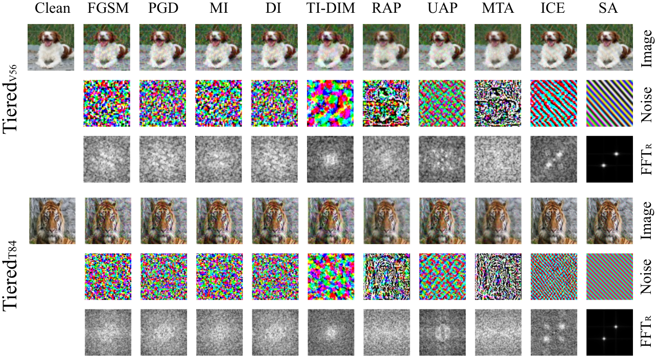
We visualize generated adversarial examples, the noise maps, and spectrum diagrams in Fig.6. To save space, we only sample two clean images from TieredT84 and TieredV56, respectively, for visualization, and will show more visualizations in Appendix. When attacking the sampled TieredT84 image, we use Cifar-10, Cifar-100, and TieredV56 as the source datasets, and use three RN-18 respectively trained on the source datasets as the source models. When attacking the sampled TieredV56 image, we use Cifar-10, Cifar-100, and TieredT84 as the source datasets. The raw FFTR denotes the spectrum of the noise map’s R channel and Appendix will visualize FFTG and FFTB.
By analyzing both Figs.1 and 6, we conclude that the perturbation noise generated by ICE differs greatly from those generated by the other methods. Compared with other methods which use irregular noise patterns to perturb different images, ICE uses regular similar texture-like noises to perturb images from different datasets. More visualizations in Appendix will also support this phenomenon. The possible reason for this phenomenon is that ICE needs to disturb the input image without knowing any information in advance, which forces ICE to learn the perturbation pattern that correlates little with ground-truth information. In our opinion, learning a generalizable perturbation pattern may be a straightforward way for ICE to solve GTA.
The spectrum diagrams demonstrate that the main components in each ICE noise are three sine waves for R, G, and B channels. The proposed SA directly optimizes the three sine waves. The visualization shows that the optimized sine waves use similar frequencies and directions with the three sine waves in ICE noise.
8 Conclusion and future work
In this paper, we propose the Generalized Transfer Attack (GTA) setting which is more challenging and more realistic than existing adversarial attack settings. We show that although existing attacks can be modified to solve this problem, they often perform poorly when the target dataset/model is different from sources. We then propose a novel Image Classification Eraser (ICE) method and show that ICE outperforms all the baselines in generalized transfer attack. More importantly, visualization and fast fourier transform analysis demonstrate that ICE uses similar texture-like noise pattern to perturb all images and the main components in each ICE noise are three sine waves. Inspired by this finding, we propose another novel method Sine Attack which directly optimizes three sine waves to solve the GTA problem. Experiments also demonstrate that SA outperforms comparably to ICE. Our work indicates that the three sine waves are enough and effective to perturb unknown images under the GTA setting.
References
- (1) Avishek Joey Bose, Gauthier Gidel, Hugo Berrard, Andre Cianflone, Pascal Vincent, Simon Lacoste-Julien, and William L Hamilton. Adversarial example games. Advances in neural information processing systems, 2020.
- (2) Wieland Brendel, Jonas Rauber, and Matthias Bethge. Decision-based adversarial attacks: Reliable attacks against black-box machine learning models. international conference on learning representations, 2018.
- (3) Nicholas Carlini and David Wagner. Towards evaluating the robustness of neural networks. In 2017 ieee symposium on security and privacy (sp), pages 39–57. IEEE, 2017.
- (4) Pin-Yu Chen, Huan Zhang, Yash Sharma, Jinfeng Yi, and Cho-Jui Hsieh. Zoo: Zeroth order optimization based black-box attacks to deep neural networks without training substitute models. In Proceedings of the 10th ACM workshop on artificial intelligence and security, pages 15–26, 2017.
- (5) Minhao Cheng, Thong Le, Pin-Yu Chen, Jinfeng Yi, Huan Zhang, and Cho-Jui Hsieh. Query-efficient hard-label black-box attack: An optimization-based approach. arXiv preprint arXiv:1807.04457, 2018.
- (6) Minhao Cheng, Simranjit Singh, Patrick H. Chen, Pin-Yu Chen, Sijia Liu, and Cho-Jui Hsieh. Sign-opt: A query-efficient hard-label adversarial attack. In international conference on learning representations, 2020.
- (7) Shuyu Cheng, Yinpeng Dong, Tianyu Pang, Hang Su, and Jun Zhu. Improving black-box adversarial attacks with a transfer-based prior. pages 10932–10942, 2019.
- (8) Francesco Croce and Matthias Hein. Minimally distorted adversarial examples with a fast adaptive boundary attack. In International Conference on Machine Learning, pages 2196–2205. PMLR, 2020.
- (9) Ekin D. Cubuk, Barret Zoph, Dandelion Mane, Vijay Vasudevan, and Quoc V. Le. Autoaugment: Learning augmentation strategies from data. In Proceedings of the IEEE/CVF Conference on Computer Vision and Pattern Recognition (CVPR), June 2019.
- (10) Nilaksh Das, Madhuri Shanbhogue, Shang-Tse Chen, Fred Hohman, Siwei Li, Li Chen, Michael E Kounavis, and Duen Horng Chau. Shield: Fast, practical defense and vaccination for deep learning using jpeg compression. In Proceedings of the 24th ACM SIGKDD International Conference on Knowledge Discovery & Data Mining, pages 196–204, 2018.
- (11) Ambra Demontis, Marco Melis, Maura Pintor, Matthew Jagielski, Battista Biggio, Alina Oprea, Cristina Nita-Rotaru, and Fabio Roli. Why do adversarial attacks transfer? explaining transferability of evasion and poisoning attacks. USENIX Security Symposium, pages 321–338, 2019.
- (12) Jia Deng, Wei Dong, Richard Socher, Li-Jia Li, Kai Li, and Li Fei-Fei. Imagenet: A large-scale hierarchical image database. In IEEE conference on computer vision and pattern recognition, pages 248–255. Ieee, 2009.
- (13) Yinpeng Dong, Fangzhou Liao, Tianyu Pang, Hang Su, Jun Zhu, Xiaolin Hu, and Jianguo Li. Boosting adversarial attacks with momentum. In Proceedings of the IEEE conference on computer vision and pattern recognition, 2018.
- (14) Yinpeng Dong, Tianyu Pang, Hang Su, and Jun Zhu. Evading defenses to transferable adversarial examples by translation-invariant attacks. In Proceedings of the IEEE/CVF Conference on Computer Vision and Pattern Recognition, pages 4312–4321, 2019.
- (15) Jiawei Du, Hu Zhang, Tianyi Joey Zhou, Yi Yang, and Jiashi Feng. Query-efficient meta attack to deep neural networks. International Conference on Learning Representations, 2020.
- (16) Chelsea Finn, Pieter Abbeel, and Sergey Levine. Model-agnostic meta-learning for fast adaptation of deep networks. In International Conference on Machine Learning, pages 1126–1135. PMLR, 2017.
- (17) Aditya Ganeshan, Vivek BS, and R Venkatesh Babu. Fda: Feature disruptive attack. In Proceedings of the IEEE/CVF International Conference on Computer Vision, pages 8069–8079, 2019.
- (18) Lianli Gao, Qilong Zhang, Jingkuan Song, Xianglong Liu, and Heng Tao Shen. Patch-wise attack for fooling deep neural network. In European Conference on Computer Vision, pages 307–322. Springer, 2020.
- (19) Robert Geirhos, Patricia Rubisch, Claudio Michaelis, Matthias Bethge, A. Felix Wichmann, and Wieland Brendel. Imagenet-trained cnns are biased towards texture; increasing shape bias improves accuracy and robustness. In ICLR, 2019.
- (20) Ian J Goodfellow, Jonathon Shlens, and Christian Szegedy. Explaining and harnessing adversarial examples. international conference on learning representations, 2014.
- (21) Yiwen Guo, Qizhang Li, and Hao Chen. Backpropagating linearly improves transferability of adversarial examples. In Advances in neural information processing systems 33 (NIPS 2020), 2020.
- (22) Kaiming He, Georgia Gkioxari, Piotr Dollár, and Ross Girshick. Mask r-cnn. In Proceedings of the IEEE international conference on computer vision, pages 2961–2969, 2017.
- (23) Kaiming He, Xiangyu Zhang, Shaoqing Ren, and Jian Sun. Deep residual learning for image recognition. In Proceedings of the IEEE conference on computer vision and pattern recognition, pages 770–778, 2016.
- (24) Andrew Howard, Mark Sandler, Grace Chu, Liang-Chieh Chen, Bo Chen, Mingxing Tan, Weijun Wang, Yukun Zhu, Ruoming Pang, Vijay Vasudevan, et al. Searching for mobilenetv3. In Proceedings of the IEEE/CVF International Conference on Computer Vision, pages 1314–1324, 2019.
- (25) Gao Huang, Zhuang Liu, Laurens Van Der Maaten, and Kilian Q Weinberger. Densely connected convolutional networks. In Proceedings of the IEEE conference on computer vision and pattern recognition, pages 4700–4708, 2017.
- (26) Qian Huang, Isay Katsman, Horace He, Zeqi Gu, Serge Belongie, and Ser-Nam Lim. Enhancing adversarial example transferability with an intermediate level attack. In Proceedings of the IEEE/CVF International Conference on Computer Vision, pages 4733–4742, 2019.
- (27) Zhichao Huang and Tong Zhang. Black-box adversarial attack with transferable model-based embedding. International Conference on Learning Representations, 2020.
- (28) Andrew Ilyas, Logan Engstrom, Anish Athalye, and Jessy Lin. Black-box adversarial attacks with limited queries and information. In International Conference on Machine Learning, pages 2137–2146. PMLR, 2018.
- (29) Andrew Ilyas, Shibani Santurkar, Dimitris Tsipras, Logan Engstrom, Brandon Tran, and Aleksander Madry. Adversarial examples are not bugs, they are features. arXiv preprint arXiv:1905.02175, 2019.
- (30) Nathan Inkawhich, Kevin J Liang, Jingyang Zhang, Huanrui Yang, Hai Li, and Yiran Chen. Can targeted adversarial examples transfer when the source and target models have no label space overlap? arXiv preprint arXiv:2103.09916, 2021.
- (31) Xu Kaidi, Liu Sijia, Zhao Pu, Chen Pin-Yu, Zhang Huan, Fan Quanfu, Erdogmus Deniz, Wang Yanzhi, and Lin Xue. Structured adversarial attack: Towards general implementation and better interpretability. International Conference on Learning Representations, 2019.
- (32) Alex Krizhevsky, Geoffrey Hinton, et al. Learning multiple layers of features from tiny images. 2009.
- (33) Alexey Kurakin, Ian Goodfellow, Samy Bengio, et al. Adversarial examples in the physical world, 2016.
- (34) Huichen Li, Xiaojun Xu, Xiaolu Zhang, Shuang Yang, and Bo Li. Qeba: Query-efficient boundary-based blackbox attack. In Proceedings of the IEEE/CVF Conference on Computer Vision and Pattern Recognition, pages 1221–1230, 2020.
- (35) Qizhang Li, Yiwen Guo, and Hao Chen. Practical no-box adversarial attacks against dnns. Advances In Neural Information Processing Systems 2020, 2020.
- (36) Yingwei Li, Song Bai, Yuyin Zhou, Cihang Xie, Zhishuai Zhang, and Alan Yuille. Learning transferable adversarial examples via ghost networks. AAAI, pages 11458–11465, 2020.
- (37) Jiadong Lin, Chuanbiao Song, Kun He, Liwei Wang, and John E Hopcroft. Nesterov accelerated gradient and scale invariance for adversarial attacks. International Conference on Learning Representations, 2020.
- (38) Tsung-Yi Lin, Priya Goyal, Ross Girshick, Kaiming He, and Piotr Dollár. Focal loss for dense object detection. In Proceedings of the IEEE international conference on computer vision, pages 2980–2988, 2017.
- (39) Tsung-Yi Lin, Michael Maire, Serge Belongie, James Hays, Pietro Perona, Deva Ramanan, Piotr Dollár, and C Lawrence Zitnick. Microsoft coco: Common objects in context. In European conference on computer vision, pages 740–755. Springer, 2014.
- (40) Hanxiao Liu, Karen Simonyan, and Yiming Yang. Darts: Differentiable architecture search. In international conference on learning representations, 2019.
- (41) Yanpei Liu, Xinyun Chen, Chang Liu, and Dawn Song. Delving into transferable adversarial examples and black-box attacks. international conference on learning representations, 2017.
- (42) Zechun Liu, Haoyuan Mu, Xiangyu Zhang, Zichao Guo, Xin Yang, Kwang-Ting Cheng, and Jian Sun. Metapruning: Meta learning for automatic neural network channel pruning. In Proceedings of the IEEE/CVF International Conference on Computer Vision, pages 3296–3305, 2019.
- (43) Yantao Lu, Yunhan Jia, Jianyu Wang, Bai Li, Weiheng Chai, Lawrence Carin, and Senem Velipasalar. Enhancing cross-task black-box transferability of adversarial examples with dispersion reduction. In Proceedings of the IEEE/CVF Conference on Computer Vision and Pattern Recognition (CVPR), June 2020.
- (44) Andriushchenko Maksym, Croce Francesco, Flammarion Nicolas, and Hein Matthias. Square attack: a query-efficient black-box adversarial attack via random search. european conference on computer vision, pages 484–501, 2020.
- (45) Nikhil Mishra, Mostafa Rohaninejad, Xi Chen, and Pieter Abbeel. A simple neural attentive meta-learner. international conference on learning representations, 2018.
- (46) Seyed-Mohsen Moosavi-Dezfooli, Alhussein Fawzi, Omar Fawzi, and Pascal Frossard. Universal adversarial perturbations. In Proceedings of the IEEE conference on computer vision and pattern recognition, 2017.
- (47) Seyed-Mohsen Moosavi-Dezfooli, Alhussein Fawzi, and Pascal Frossard. Deepfool: a simple and accurate method to fool deep neural networks. In Proceedings of the IEEE conference on computer vision and pattern recognition, pages 2574–2582, 2016.
- (48) Muhammad Muzammal Naseer, Salman H Khan, Muhammad Haris Khan, Fahad Shahbaz Khan, and Fatih Porikli. Cross-domain transferability of adversarial perturbations. Advances in Neural Information Processing Systems, 32:12905–12915, 2019.
- (49) Inkawhich Nathan, Kevin Liang J, Wang Binghui, Inkawhich Matthew, Carin Lawrence, and Chen Yiran. Perturbing across the feature hierarchy to improve standard and strict blackbox attack transferability. In NIPS, 2020.
- (50) Nicolas Papernot, Patrick McDaniel, and Ian Goodfellow. Transferability in machine learning: from phenomena to black-box attacks using adversarial samples. arXiv preprint arXiv:1605.07277, 2016.
- (51) Nicolas Papernot, Patrick McDaniel, Ian Goodfellow, Somesh Jha, Z Berkay Celik, and Ananthram Swami. Practical black-box attacks against machine learning. In Proceedings of the 2017 ACM on Asia conference on computer and communications security, pages 506–519, 2017.
- (52) Aditya Prakash, Kashyap Chitta, and Andreas Geiger. Multi-modal fusion transformer for end-to-end autonomous driving. In Proceedings of the IEEE/CVF Conference on Computer Vision and Pattern Recognition, pages 7077–7087, 2021.
- (53) Yunxiao Qin, Yuanhao Xiong, Jinfeng Yi, and Cho-Jui Hsieh. Training meta-surrogate model for transferable adversarial attack. arXiv preprint arXiv:2109.01983, 2021.
- (54) Yunxiao Qin, Zitong Yu, Longbin Yan, Zezheng Wang, Chenxu Zhao, and Zhen Lei. Meta-teacher for face anti-spoofing. IEEE Transactions on Pattern Analysis and Machine Intelligence, pages 1–1, 2021.
- (55) Yunxiao Qin, Weiguo Zhang, Zezheng Wang, Chenxu Zhao, and Jingping Shi. Layer-wise adaptive updating for few-shot image classification. IEEE Signal Processing Letters, 27:2044–2048, 2020.
- (56) Mengye Ren, Eleni Triantafillou, Sachin Ravi, Jake Snell, Kevin Swersky, Joshua B Tenenbaum, Hugo Larochelle, and Richard S Zemel. Meta-learning for semi-supervised few-shot classification. International Conference on Learning Representations, 2018.
- (57) Mengye Ren, Wenyuan Zeng, Bin Yang, and Raquel Urtasun. Learning to reweight examples for robust deep learning. In International Conference on Machine Learning, pages 4334–4343. PMLR, 2018.
- (58) Shaoqing Ren, Kaiming He, Ross Girshick, and Jian Sun. Faster r-cnn: towards real-time object detection with region proposal networks. IEEE transactions on pattern analysis and machine intelligence, 39(6):1137–1149, 2016.
- (59) Karen Simonyan and Andrew Zisserman. Very deep convolutional networks for large-scale image recognition. International Conference on Learning Representations, 2015.
- (60) Christian Szegedy, Wojciech Zaremba, Ilya Sutskever, Joan Bruna, Dumitru Erhan, J. Ian Goodfellow, and Rob Fergus. Intriguing properties of neural networks. international conference on learning representations, 2014.
- (61) Florian Tramèr, Alexey Kurakin, Nicolas Papernot, Ian Goodfellow, Dan Boneh, and Patrick McDaniel. Ensemble adversarial training: Attacks and defenses. arXiv preprint arXiv:1705.07204, 2017.
- (62) C. Wah, S. Branson, P. Welinder, P. Perona, and S. Belongie. The Caltech-UCSD Birds-200-2011 Dataset. Technical Report CNS-TR-2011-001, California Institute of Technology, 2011.
- (63) Lu Wang, Huan Zhang, Jinfeng Yi, Cho-Jui Hsieh, and Yuan Jiang. Spanning attack: reinforce black-box attacks with unlabeled data. Machine Learning, 109(12):2349–2368, 2020.
- (64) Xiaosen Wang and Kun He. Enhancing the transferability of adversarial attacks through variance tuning. In Proceedings of the IEEE/CVF Conference on Computer Vision and Pattern Recognition, pages 1924–1933, 2021.
- (65) Xin Wang, Jie Ren, Shuyun Lin, Xiangming Zhu, Yisen Wang, and Quanshi Zhang. A unified approach to interpreting and boosting adversarial transferability. International Conference on Learning Representations, 2021.
- (66) Dongxian Wu, Yisen Wang, Shu-Tao Xia, James Bailey, and Xingjun Ma. Skip connections matter: On the transferability of adversarial examples generated with resnets. international conference on learning representations, 2020.
- (67) Kaiwen Wu, Allen Wang, and Yaoliang Yu. Stronger and faster wasserstein adversarial attacks. International Conference on Machine Learning, pages 10377–10387, 2020.
- (68) Lei Wu, Zhanxing Zhu, Cheng Tai, et al. Understanding and enhancing the transferability of adversarial examples. arXiv preprint arXiv:1802.09707, 2018.
- (69) Weibin Wu, Yuxin Su, Xixian Chen, Shenglin Zhao, Irwin King, R. Michael Lyu, and Yu-Wing Tai. Boosting the transferability of adversarial samples via attention. In Proceedings of the IEEE/CVF Conference on Computer Vision and Pattern Recognition, pages 1158–1167, 2020.
- (70) Zang Xiao, Xie Yi, Chen Jie, and Yuan Bo. Graph universal adversarial attacks - a few bad actors ruin graph learning models. International Joint Conference on Artificial Intelligence, pages 3328–3334, 2021.
- (71) Cihang Xie, Zhishuai Zhang, Yuyin Zhou, Song Bai, Jianyu Wang, Zhou Ren, and Alan L Yuille. Improving transferability of adversarial examples with input diversity. In Proceedings of the IEEE/CVF Conference on Computer Vision and Pattern Recognition, pages 2730–2739, 2019.
- (72) Dong Yin, Raphael Gontijo Lopes, Jon Shlens, Ekin Dogus Cubuk, and Justin Gilmer. A fourier perspective on model robustness in computer vision. In Advances in Neural Information Processing Systems, volume 32, 2019.
- (73) Zheng Yuan, Jie Zhang, Yunpei Jia, Chuanqi Tan, Tao Xue, and Shiguang Shan. Meta gradient adversarial attack. In Proceedings of the IEEE/CVF International Conference on Computer Vision, 2021.
- (74) Chaoning Zhang, Philipp Benz, Adil Karjauv, and In So Kweon. Data-free universal adversarial perturbation and black-box attack. In Proceedings of the IEEE/CVF International Conference on Computer Vision, pages 7868–7877, 2021.
- (75) Chaoning Zhang, Philipp Benz, Adil Karjauv, and In So Kweon. Universal adversarial perturbations through the lens of deep steganography: Towards a fourier perspective. In Proceedings of the AAAI Conference on Artificial Intelligence, volume 35, pages 3296–3304, 2021.
- (76) Wen Zhang, Yang Feng, Fandong Meng, Di You, and Qun Liu. Bridging the gap between training and inference for neural machine translation. In 57th annual meeting of the association for computational linguistics (ACL 2019), pages 4334–4343, 2019.
- (77) Wen Zhou, Xin Hou, Yongjun Chen, Mengyun Tang, Xiangqi Huang, Xiang Gan, and Yong Yang. Transferable adversarial perturbations. In Proceedings of the European Conference on Computer Vision (ECCV), pages 452–467, 2018.
Appendix A Network architecture of ICE
As mentioned in Section 4 of the main body, the proposed ICE should be able to handle images with different resolutions because we cannot know the image shape in advance. Therefore, we build a fully convolutional neural network shown in Figure 7 as the backbone of ICE. The parameters , , , and are set to 32, 64, 128, and 256, respectively.
Appendix B More details of TieredT84 and TieredV56
For either TieredT84 or TieredV56, we use the image ID to rank all images of each category and use the first 1200 images of each category to compose the training set and use the last 100 images to compose the testing set. For example, the IDs of the two images ‘n01530575_5.JPEG’ and ‘n01530575_23.JPEG’ from the ‘n01530575’ category are 5 and 23.
Appendix C Training details of source and target models
On each of the datasets Cifar-10, Cifar-100, TieredT84, and TieredV56, we train the four models RN-18, VGG-16, MB-V3, and DN-26. The network architectures of all the four models are defined in the public GitHub repository22 2 https://github.com/yxlijun/cifar-tensorflow. We use consistent hyper-parameters to train all the models for 80,000 iterations without data augmentation. The learning rate, L2 weight decay, and batch size are set to 0.01, 1e-5, and 128, respectively. Table 9 shows the four models’ accuracies on the four datasets.
| Dataset | MB-V3 | VGG-16 | RN-18 | DN-26 |
|---|---|---|---|---|
| Cifar-10 | 80.0% | 92.9% | 91.8% | 91.2% |
| Cifar-100 | 43.9% | 68.5% | 68.0% | 64.6% |
| TieredT84 | 35.3% | 46.9% | 47.0% | 44.6% |
| TieredV56 | 32.1% | 46.3% | 45.9% | 46.0% |
Appendix D Additional experiments
D.1 Output dimension of ICE
We set the output dimension of ICE as 1,000 by default. Here we show how the output dimension affects the results in Figure 8(a). We can see that the average attack success rates on the four target models will rise when the output dimension is increased from 30 to 300, and will become stable when the output dimension 300.
D.2 Customized FGSM or Customized PGD?
Eq.2 in the main body shows that we use Customized FGSM to perturb the input image in the inner-loop. We conduct an experiment to show why we use Customized FGSM instead of Customized PGD qin2021training. Customized PGD is a multi-step Customized FGSM. In this experiment, we increase the number of gradient ascent steps from 1 to 5. Figure 8(b) shows the experimental results. It is clear that the performance of ICE will be damaged by the increase of the number of gradient ascent steps. The possible reason for this phenomenon is that multi-step gradient ascent in the inner-loop makes the model hard to be optimized in the outer-loop.
D.3 Attacking robust models
Here we conduct generalized transfer attack on robust models. In this experiment, we use RN-18 and Cifar-10 as the source model and the source dataset, and disturb the images from Cifar-100. The target models are adversarially trained RN-18 and RN-34 on Cifar-100, which can be denoted as RN-18adv and RN-34adv, respectively. To obtain RN-18adv, we firstly use the normally trained RN-18 to generate adversarial examples for all training examples with FGSM (=15), and then retrain RN-18 on all the clean training images and the adversarial images. We obtain RN-34adv in a similar way. The two models finally achieve approximately 46.9% and 47.3% testing accuracies on Cifar-100. The generalized transfer attack results on RN-18adv and RN-34adv are reported in Table 10. Obviously, though all the methods perform not well to attack adversarially trained models, ICE and SA still show their advantages in this experiment.
D.4 Re-implement PGD-based baselines with KL divergence
In the main body, the PGD-based baselines disturb input images by maximizing the entropy loss of source models. Here we re-implement PGD-based baselines with KL divergence, which means the baselines disturb the input images by maximizing the KL divergence between the predicted distribution and , where is the predicted distribution for the original clean image . Then the perturbation generated in each gradient ascent step can be reformulated as . In this experiment, we use RN-18 and Cifar-10 as the source model and source dataset, and use Cifar-100 as the target dataset. The generalized transfer attack results on MB-V3, VGG-16, RN-18, and DN-26 are reported in Table 11. The comparison between the results here and those in Table 2 demonstrates that the KL divergence cannot improve PGD-based baselines.
| Resource | Method | RN-18adv | RN-34adv |
|---|---|---|---|
| Cifar-10 (RN-18) | FGSM | 11.1% | 12.9% |
| PGD | 9.7% | 10.1% | |
| DI | 11.0% | 11.6% | |
| MI | 10.8% | 11.8% | |
| TI-DIM | 16.7% | 15.9% | |
| IR | 13.8% | 13.1% | |
| UAP | 11.2% | 11.8% | |
| RAP | 14.9% | 16.0% | |
| ICE | 17.3% | 17.8% | |
| SA | 16.0% | 18.8% |
| Resource | Method | MB-V3 | VGG-16 | RN-18 | DN-26 |
|---|---|---|---|---|---|
| Cifar-10 (RN-18) | FGSM | 49.3% | 63.3% | 57.9% | 72.5% |
| PGD | 39.6% | 52.5% | 45.0% | 62.7% | |
| DI | 41.2% | 54.6% | 46.5% | 64.2% | |
| MI | 47.3% | 62.6% | 56.9% | 72.4% | |
| TI-DIM | 50.6% | 43.1% | 45.6% | 52.4% |
| Resource | Method | MB-V3 | VGG-16 | RN-18 | DN-26 |
|---|---|---|---|---|---|
| Cifar-10 + TieredT84 + TieredV56 (RN-18) | FGSM | 47.5% | 63.2% | 56.3% | 72.6% |
| PGD | 38.8% | 53.6% | 43.1% | 64.6% | |
| DI | 38.6% | 53.9% | 43.3% | 64.7% | |
| MI | 46.2% | 62.8% | 53.8% | 71.9% | |
| TI-DIM | 47.9% | 43.8% | 44.9% | 54.0% |
D.5 Optimizing a single adversarial image
In our previous experiments, we implement PGD-based baselines with the pipeline introduced in Section 6.1, where we firstly optimize the adversarial example for each source model respectively and then obtain the final adversarial example by fusing all the adversarial examples. Here we re-implement PGD-based baselines with a new pipeline, where we directly optimize a single adversarial image for all source models. The new pipeline uses gradient ascent iterations to disturb the input image, and the -th iteration contains the following three steps.
1) Suppose is the perturbed image generated in the iteration and . We resize the image to the input shapes of all source models and then feed the resized images to the source models, respectively. Then the inference of on one source model can be formulated as , where is the resized image for the source model .
2) We calculate the prediction losses of all the source models with the formulation , where is entropy.
3) We disturb the input image with the formulation , where .
After iterations, we obtain the disturbed image , and generate the final adversarial image by . Then we feed both and the clean image into the unknown target model and get the predictions. The GTA process is successful if .
We conduct an experiment to evaluate how the re-implemented PGD-based baselines perform on GTA. In this experiment, Cifar-10, TieredT84, and TieredV56 are used as source datasets, and three RN-18 respectively trained on the three datasets are used as the source models. The experimental results on the target models MB-V3, VGG-16, RN-18, and DN-26 are reported in Table 12. Compared with the results in the last row of Table 2, optimizing a single image improves FGSM and MI, but damages DI and TI-DIM.
The possible reason for this result is that there still exists implicit resizing operations when we optimize a single adversarial image (the gradient propagates through resizing layers) at each gradient ascent step.
Suppose there are three source models respectively trained on TieredT84, TieredV56, and Cifar-10. With the three source datasets, each gradient ascent step needs 3 explicit and 3 implicit resizing operations in the forward and backward paths, respectively. Optimizing a single adversarial image needs to fuse the gradients from all the three source models at each gradient ascent step. This may result in the single adversarial example obtained in the step being not optima and accurate to attack each source model due to the implicit resizing operations, and further influences the following gradient ascent steps. As introduced in Section 6.1, the default implementation of baselines explicitly resizes the adversarial images only before the first and only after the last gradient ascent steps. For example, when using the Cifar-10 model to generate the perturbation, we explicitly resize the image to the resolution of Cifar-10 model only before the first gradient ascent step, and explicitly resize the adversarial example on the Cifar-10 model back into the original resolution of only after the last gradient ascent step. Therefore, between the first and the last step, there are no resizing operations to influence the adversarial effectiveness of the adversarial examples generated on the Cifar-10, TieredT84, and TieredV56 models, respectively.
The experiment shows that FGSM can be improved by optimizing a single adversarial image, which may prove the above reason. FGSM contains a single gradient ascent step, which means the first and the last gradient ascent steps is the same. When optimizing a single adversarial image, FGSM has 3 implicit and 3 explicit resizing operations, while when using the default implementation introduced in Section 6.1, FGSM contains 32=6 explicit resizing operations. In our opinion, gradient fusing through implicit resizing operations is more accurate than through explicit resizing operations, and this is the reason why FGSM can be improved by optimizing a single adversarial image.
The experiment also shows that PGD can be damaged by optimizing a single adversarial image. PGD contains 10 gradient ascent steps in our work. When optimizing a single adversarial image, PGD has 310=30 implicit and 310=30 explicit resizing operations, while when using the default implementation introduced in Section 4.1, PGD contains only 32=6 explicit resizing operations. In our opinion, the more the number of explicit resizing operations, the worse the GTA performance, and this is the reason why optimizing a single adversarial image at each gradient ascent step damages PGD.
D.6 Using Knowledge distillation to train a single model
In this experiment, we use Cifar-10, TieredT84, and TieredV56 as source datasets, and use three RN-18 respectively trained on the source datasets as source models. First, we build another model that has three heads that correspond to the three source datasets. The backbone of is the same with that of the proposed ICE. The first head that has 10 output nodes is used to classify Cifar-10 images. The second head which has 351 output nodes is used to classify TieredT84 images. The third head which has 257 output nodes is used to classify TieredV56 images. Second, we use the three source models and three datasets to train a student model with offline knowledge distillation. The student model obtain test accuracies of 97.5%, 61.7%, and 70.3% on Cifar-10, TieredT84, and TieredV56, respectively. Finally, we use the student model to disturb the images from Cifar-100. The GTA success rates on the target models MB-V3, VGG-16, RN-18, and DN-26 are reported in Table 13. The comparison between the results in Table 13 with those in the last row of Table 2 (in the main body) indicates that attacking a single student model cannot improve the GTA performances.
| Method | MB-V3 | VGG-16 | RN-18 | DN-26 |
|---|---|---|---|---|
| FGSM | 46.4% | 59.6% | 51.0% | 70.6% |
| PGD | 36.9% | 49.6% | 40.3% | 61.3% |
| MI | 43.9% | 56.6% | 47.6% | 68.4% |
Appendix E Computational cost
We conduct all experiments on Tesla P40 GPU. The training cost of the proposed ICE is determined by the backbone, the used source datasets, the source models, and etc.. The number of parameters of ICE is determined by the backbone. The backbone which contains about 7.7M parameters is shown in Figure 7. With the source datasets Cifar-10, TieredT84, and Tiered56, and with the three corresponding RN-18 source models, training the model costs about 1.3T FLOPs per iteration when batch size=64.
In inference, the cost of ICE is determined by the backbone, the size of the testing image, and the number of gradient ascent step , which is set to 10 in our work. The inference costs of PGD-based baselines depend on the size of the testing image, the source models, and the number of gradient ascent steps . When the testing image comes from Cifar-100, ICE costs approximately 1.2G FLOPs per gradient ascent step per image, while the PGD-based baseline MI, DI, or TI-DIM costs approximately 10.2G FLOPs, which indicates that ICE is much more efficient than PGD-based baselines in inference.
The training cost of the proposed SA is determined by the used source datasets, the source models, and etc.. With the source datasets Cifar-10, TieredT84, and Tiered56, and with the three corresponding RN-18 source models, training the parameter costs about 0.77T FLOPs per iteration when batch size=64.
In inference, the cost of SA is almost zero because SA perturb the clean image by directly adding the noise to the clean image. As a comparison, the baselines RAP and AEG need to firstly generate the adversarial perturbation via generators before adding the perturbation to the clean image. Similarly, the baseline UAP needs resizing the trained universal perturbation before adding the resized perturbation to the clean image.
In conclusion, in terms of GTA performance, the proposed ICE and SA perform almost comparable and both of them greatly outperform the baselines, and in terms of efficiency, the proposed SA performs the best among all methods because its inference cost is almost zero.
Appendix F More analysis about SP
The ablation study shown in Section 6.8 demonstrates that the trick SP in this paper is important for ICE and PGD-based baselines to achieve better generalized transferable attack success rates. It is also observed that without SP, MI performs the best among ICE and all PGD-based baselines. This is because MI utilizes gradient momentum to improve the attack success rate, and the momentum will enlarge the average perturbation scale of each pixel while keeping the of the perturbation map unchanged, which plays a similar role to SP. For instance, without SP, the average perturbation scale of each pixel of the adversarial examples generated via MI is approximately 11. As a comparison, for the other PGD-based methods and ICE, the average perturbation scale of each pixel of the generated adversarial examples is no more than 9.
Appendix G More visualizations of noises and spectrum diagrams
In Fig.9, we visualize more generated adversarial examples, the corresponding noise maps, and spectrum diagrams. Four datasets Cifar-10, Cifar-100, TieredV56, and TieredT84 are used for the visualization. For each dataset, we randomly sample a clean image for visualization and use the other three datasets as the source datasets. For example, when we sample the clean image from TieredT84 for visualization, the source datasets are Cifar-10, Cifar-100, and TieredV56, and the source models are three RN-18 respectively trained on the source datasets. Each raw FFTx, where [R, G, B], denotes the spectrum diagram of the noise map’s channel. All the visualizations support the phenomenon that compared with the other methods, ICE noise is more regular, and the main components in ICE noise are three sine functions. We propose the SA method to directly optimize the three sine waves and further demonstrate that the three sine functions are enough and effective to break DNNs under the GTA setting. The frequency of each sine wave is , and the wave direction is arctan(). In experiments, we found that the frequencies of the three optimized sine waves are commonly around 0.18HZ, and the directions of the three sine waves are commonly around .
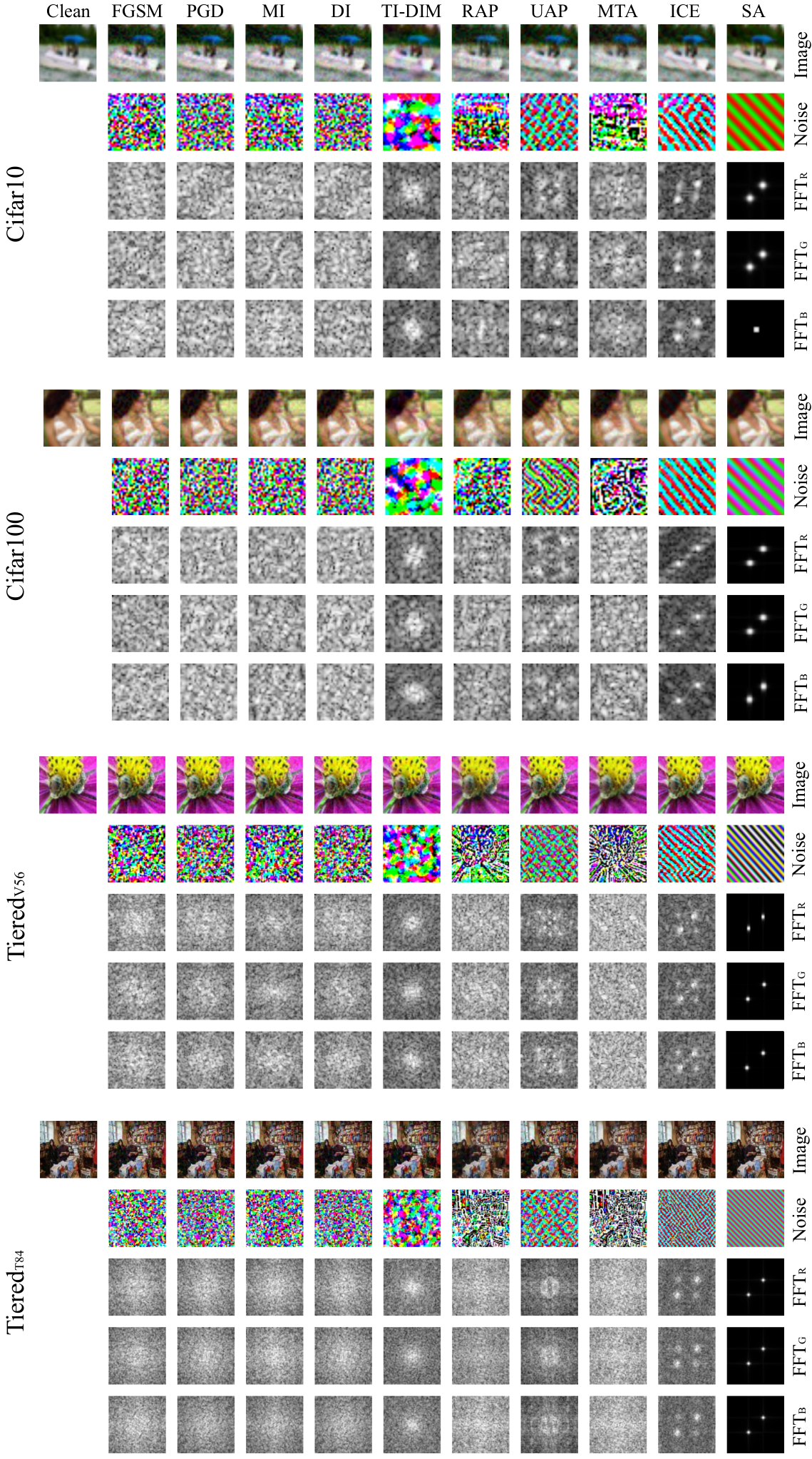
Appendix H Visualization of perturbed MS-COCO images
Here we visualize a clean MS-COCO image and the corresponding adversarial images generated by PGD, DI, TI-DIM, UAP, RAP, MTA, ICE, and SA, in Fig.10. The bounding boxes predicted by Faster-RCNN are also visualized for readers to better understand how Faster-RCNN predicts the adversarial examples. is set to 15. The source datasets are Cifar-10, TieredT84, and TieredV56, and the source models are three ResNet-18 models respectively trained on the three source datasets. Obviously, among all methods, SA performs the best to perturb MS-COCO images because Faster-RCNN can only detect three objects on the adversarial image generated by SA but can detect more objects on the other adversarial images.

Appendix I Additional implementation details of baselines
Some implementation details of baselines have been introduced in Section 6.1 of the main body. Here we introduce additional implementation details of baselines.
MI: Parameter of MI dong2018boosting is set to 1.
DI:. We use the code33 3 https://github.com/cihangxie/DI-2-FGSM to implement DI xie2019improving in all our experiments. We set ’FLAGS.image_resize’ to 36, 64, or 96, when the resolution of the input image is 32, 56, or 84, respectively. The input diverse possibility is set to 1.0.
TI-DIM:. We use the code44 4 https://github.com/dongyp13/Translation-Invariant-Attacks to implement TI-DIM dong2019evading in all our experiments.
IR:. We use the code55 5 https://github.com/xherdan76/A-Unified-Approach-to-Interpreting-and-Boosting-Adversarial-Transferability to implement IR wu2020skip in all our experiments. The hyper-parameter ‘args.grid_scale’ and ‘args.sample_grid_num’ are set to 1 and 16, respectively, for all experiments.
FDA+xent:. We refer to the FDA+xent paper nathan2020perturbing to implement it on the generalized transferable attack problem. Given the RN-18 source model, we train auxiliary binary classifiers based on the third block feature. is the number of classes of the RN-18 model. Each auxiliary classifier contains two hidden layers with each layer containing 100 neurons. Then, we use the FDA+xent optimizing objective to disturb the auxiliary classifiers and the middle-layer features, and generate perturbation noises for input images following the pipeline introduced in Section 6.1.1.
AEG. We implement AEG bose2020adversarial in our experiment by referring to the code66 6 https://github.com/joeybose/Adversarial-Example-Games. Given each source dataset and the corresponding source models trained on it, we adversarially train a perturbation generator together with a critic. The generator can be denoted as . For example, for the experiment scene ‘-Cifar-10’, we train three generators on the three source datasets Cifar-100, TieredT84 and TieredV56, and denote them as , , , respectively. The architecture of all generators is the encoder-decoder defined in Tab.7 of AEG’s paper. Note that considering ground-truth label is unavailable in GTA’s inference phase, we do not use the label as the additional input signal for the decoder when training the generators. Each generator’s input-size is the same with the image-shape of the corresponding training dataset. On either Cifar-10 or Cifar-100, we train the generator and the critic for 500 epochs with the learning rate of 0.001. On either TieredT84 or TieredV56, we train the generator and the critic for 120 epochs with the learning rate of 0.001.
In the inference phase, we use the following steps to evaluate AEG on generalized transferable attack. 1) For each generator , we resize the testing clean image to the input shapes of the generator, which can be formulated as , and then feed the resized image to the generator . 2) Obtain the perturbation generated by each generator, which can be formulated as . 3) Average fuse all the perturbations generated by all generators with the formulation , where is the number of generators. 4) Obtain the adversarial example , where is default set to 15. 5) Feed and into the unknown target model , and get the predictions. 6) The generalized transferable attack is successful if .
MTA. We refer to the MTA paper qin2021training to implement it on the generalized transferable attack problem. Given each source dataset and the corresponding source models trained on it, we train a meta-surrogate model, which can be denoted as . Each meta-surrogate model’s input-size is the same with the image-shape of the training dataset. We train the meta-surrogate models on all the source datasets with the following settings. On either Cifar-10 or Cifar-100, we train the meta-surrogate model for 50,000 iterations with the parameter and number of attack steps (in Customized PGD) set to 1600 and 7, respectively. On either TieredT84 or TieredV56, we train the meta-surrogate model for 70,000 iterations with the parameter and number of attack steps set to 2100 and 4, respectively. On each training dataset, is exponentially decayed by 0.9 for every 4000 iterations. The learning rate and the batch size are set to 0.001 and 64, respectively.
We use the following steps to evaluate MTA on generalized transferable attack. 1) For each meta-surrogate model , we resize the testing clean image to the input shape of , which can be formulated as . 2) We then feed the resized image to the meta-surrogate model . Because we cannot access the category of the image in advance, no ground-truth label can be leveraged to perturb the resized image . Therefore, for each meta-surrogate model , we generate adversarial example for by maximizing the entropy (as used in our ICE) for gradient ascent steps. The -th step can be formulated as
| (14) |
where is the meta-surrogate model’s output. and are the adversarial example and the perturbation generated in the -th step, respectively. 3) Resize the adversarial example generated by the meta-surrogate model to the original shape of the image , which can be formulated as . 4) Average fuse the adversarial examples generated by all meta-surrogate models to one image following the formulation , where is the number of meta-surrogate models. 5) Generate adversarial example by the formulation , which is the SP step defined in Section 4.2 of the main-body. 6) Feed the adversarial example and the clean image into the unknown target model and get the predictions. 7) The GTA process is successful if .
UAP. The original UAP zhang2021data constructs a universal perturbation within a single dataset. However, the GTA setting requires the perturbation to be generalized to unknown dataset. So we re-implement UAP under the GTA setting by Algorithm 3. We set the initial resolution of the UAP to 100100, and before using it to attack each victim image, we resize it to the resolution of the victim image (See Resize in line 4 of Algorithm 3). The obtained adversarial examples are denoted as . , the batch size, and the learning rate are set to 15, 128, and 0.01, respectively. We train UAP for totally 40,000 iterations.
Given any clean image that will be fed into an unknown target model , we evaluate the trained UAP with the following steps. 1) Resize to the resolution of . 2) Generate the adversarial example by the formulation
| (15) |
3) Feed the adversarial example and the clean image into the unknown target model and get its predictions and . 4) The GTA process is successful if .
input: Source datasets , Source models for each dataset , Initial perturbation with size of 100100.
output: Optimized perturbation .
1 : while not done do
2 : for each do
3 : Sample a mini data batch
4 :
5 : for each do
6 : Obtain loss on via Eq.10 of main-body.
7 : end for
8 : end for
9 :
10: end while
11: return
RAP. We implement RAP naseer2019cross-domain in our work by referring to the official paper and code77 7 https://github.com/Muzammal-Naseer/Cross-Domain-Perturbations. Given each source dataset and the corresponding source models trained on it, we train a perturbation generator following Algorithm 1 in RAP’s official paper. The generator can be denoted as . For example, for the experiment scene ‘-Cifar-10’, we train three generators on the three source datasets Cifar-100, TieredT84 and TieredV56, and denote them as , , , respectively. The architecture of all generators is the encoder-decoder defined in RAP’s official code (‘generators.py’ file). Each generator’s input-size is the same with the image-shape of the corresponding training dataset. After training the generators, we use the evaluation pipeline of AEG to evaluate RAP under the GTA setting.