A data-driven model reduction method for parabolic inverse source problems and its convergence analysis
Abstract
In this paper, we propose a data-driven model reduction method to solve parabolic inverse source problems efficiently. Our method consists of offline and online stages. In the off-line stage, we explore the low-dimensional structures in the solution space of the parabolic partial differential equations (PDEs) in the forward problem with a given class of source functions and construct a small number of proper orthogonal decomposition (POD) basis functions to achieve significant dimension reduction. Equipped with the POD basis functions, we can solve the forward problem extremely fast in the online stage. Thus, we develop a fast algorithm to solve the optimization problem in the parabolic inverse source problems, which is referred to as the POD algorithm in this paper. Under a weak regularity assumption on the solution of the parabolic PDEs, we prove the convergence of the POD algorithm in solving the forward parabolic PDEs. In addition, we obtain the error estimate of the POD algorithm for parabolic inverse source problems. Finally, we present numerical examples to demonstrate the accuracy and efficiency of the proposed method. Our numerical results show that the POD algorithm provides considerable computational savings over the finite element method.
AMS subject classification: 35R30, 65J20, 65M12, 65N21, 78M34.
Keywords: Parabolic inverse source problems; regularization method; data-driven model reduction; proper orthogonal decomposition (POD); stochastic error estimate; optimal regularization parameter.
1 Introduction
This paper presents a data-driven model reduction method to solve parabolic inverse source problems and studies the convergence analysis of the proposed method. Inverse problems are very important in physics, engineering, and bioengineering. The inverse source problems, which seeks reconstruction of source from final time observation, have attached much attention of the researchers over the past decades, see an introduction and references in [21]. They have been widely studied in the literature, applied to many physical and engineering source identification problems, e.g. migration of groundwater, groundwater pollution detection, control of pollution source and environmental protection [8, 12, 15, 11, 20] and references therein. The accurate recovery pollutant source is crucial to environmental safeguard in cities with high populations [9]. The estimation of the strength of acoustic sources from measurements can be found in e.g. [20, 13, 27]. The inverse source problems that arise from PDEs are ill-posed in the sense of Isakov and Hadamard [20, 17], since the eigenvalues of the elliptic operators decay exponentially fast, especially the lack of stability with respect to the uncertainty in the measurement data is the most difficult challenge for numerical inversions. Namely, a small change in the data may lead to a significant difference in the reconstructed source strength. Due to the important applications of inverse source problems, numerical methods have been widely explored [8, 7, 26, 14, 15] and references can be found therein.
In this paper, we will work on a very practically physical scenario, assuming that the observational measurement is collected point-wisely over a set of distributed sensors located at over the physical domain [11, 20, 25, 28]. At each sensor, independently additional noise or random error will be considered due to the uncertainty of natural noise, measurement errors, and the other uncertainty of the model itself. We will take one of the realistic approaches for such inverse problems, i.e. optimizing the mean-square error with a proper Tikhonov type regularizations [7, 15, 35]. Classical methods such as regression methods [15], linear and nonlinear programming methods [15], linear and nonlinear conjugate gradient methods [1, 35], Newton-type methods, etc. can be applied during optimization. For the inverse parabolic source problem, one usually uses iteration optimization methods to find the true source term [7, 10, 22]. In each iteration, one has to solve the forward parabolic equation one or two times. However, as the sizes of discrete problems grow (e.g. finite element method (FEM) or finite difference method (FDM)), the computation time will grow rapidly, especially for such evolution problems. As a consequence, the computation of the forward equation will cost the most time throughout the whole procedure. This motivates us to develop efficient model reduction methods to address this issue.
One of the successful model reduction ideas in solving evolution problems is the proper orthogonal decomposition (POD) method [31, 5]. The POD method uses the data from an accurate numerical simulation and extracts the most energetic modes in the system by using the singular value decomposition. This approach generates low-dimensional structures that can approximate the solutions of the evolution problems with high accuracy. The POD method has been used to solve many types of PDEs, including linear parabolic equations [34], Navier‐Stokes equations [23], viscous G-equations [16], Hamilton–Jacobi–Bellman (HJB) equations [24], and optimal control problem [2]. The interested reader is referred to [29, 3, 18] for a comprehensive introduction of the model reduction methods.
Since the POD method can significantly accelerate the computation of the forward problem compared with the traditional methods, e.g. FEM and FDM, we apply the POD method to solve parabolic inverse source problems with scattered measured data at the final time. The key idea is to exploit (model-based) and construct (data-based) the intrinsic approximate low-dimensional structures of the underlying problem that consists of two components. First, we have a training component that computes a set of data-driven basis functions (i.e. the POD basis functions) to achieve significant dimension reduction in the solution space. Following up, there is a fast-solving component that solves the optimization problem using the constructed POD basis functions in each iteration. Hence we achieve an effective data-driven model reduction method in solving the parabolic inverse source problems and overcome the typical computational bottleneck in the traditional methods, e.g. FEM and FDM.
Then, we study the convergence analysis of the proposed method. In [7], a general theory of the stochastic convergence of numerical method has been established for a certain type of inverse problem. Based on this framework, we explore the convergence theory in the POD settings. Specifically, we will prove a relatively weaker convergence of the POD method when the source term only belongs to , where is the computational domain. Unlike the traditional analysis of the POD method [23] or FEM convergence, we do not assume the higher regularity for parabolic PDE solution , i.e. to be bounded in , which is quite strict in many cases. Based on our analysis, we derive the stochastic convergence when applying the POD method to the parabolic inverse source problem with uncertain data. Our analysis in Theorem 4.3 shows that the optimal error of the Tikhonov type least-square optimization problem depends on the noise level, the number of sensors, and without any higher source regularization but the norm of the source term. A self-consistent algorithm to get the optimal smoothing parameter is also established using the POD method to solve the inverse parabolic source problem, motivated by the recent study in [6, 7]. Finally, we conduct numerical experiments to demonstrate the accuracy and efficiency of the proposed method. Several kinds of source functions are involved. Comparing to original optimization with FEM basis functions, the proposed POD method significantly reduces the computational cost and maintains the same accuracy as the FEM.
The rest of the paper is organized as follows. In Section 2, we introduce the setting of the parabolic inverse source problems. In Section 3, we develop the data-driven model reduction method for solving parabolic inverse source problems. In Section 4, we provide the error estimate for the proposed method. In Section 5, we present numerical results to demonstrate the accuracy of our method. Finally, concluding remarks are made in Section 6.
2 Parabolic inverse source problems
To start with, we consider a parabolic equation,
| (2.1) |
where is a bounded domain with boundary or a convex domain satisfying the uniform cone condition, is a second-order elliptic operator given by , and is the initial value. We assume the elliptic operator is uniform elliptic, i.e. there exist , such that for all . Moreover, we assume , and .
Let be the solution of the parabolic equation (2.1). We define the forward operator by . The forward problem is to compute the solution for with known source term and known initial condition .
In the parabolic inverse source problem, is an unknown source term that we want to reconstruct based on the final time measurement . To be specific, we will focus on a very practically physical scenario, where we assume that the observational measurement is collected point-wisely over a set of distributed sensors located at over the physical domain (see e.g.[11, 20, 25, 28]). We also assume the measurement data is always blurred by noise and takes the form , , where is the true source term and are independent and identically distributed (i.i.d.) random variables on a proper probability space (. From [7] and the analysis therein, we know that . According to the embedding theorem of Sobolev spaces, we know that is continuously embedded into so that is well defined point-wisely for all . Without loss of generality, we assume that the scattered locations are uniformly distributed in , i.e., there exists a constant such that , where and are defined by
| (2.2) |
We denote the inner product between the measurement data and any function by . Moreover, we denote the inner product between two functions by for any and the empirical norm for any .
Equipped with these definitions, we can define the parabolic inverse source problem as to recover the unknown source term from the noisy final time measurement data , . We will use the regularization method to solve this parabolic inverse source problem. Specifically, we will look for an approximate solution of the true source term by solving the following least-squares regularized minimization problem:
| (2.3) |
where is the regularization parameter.
We first recall an existing work [7], where the optimal stochastic convergence of regularized solutions and finite element solutions to time-dependent parabolic inverse source problems (2.1) have been studied. The following result represents the stochastic convergences corresponding to the random variables with bounded variance.
Proposition 2.1 (Theorem 3.4 in [7])
Suppose are independent random variables satisfying and . Let be the solution of the least-squares regularized minimization problem (2.3). Then there exist constants and such that the following estimates hold for any :
| (2.4) | |||
| (2.5) | |||
| (2.6) |
A stronger stochastic convergence when are independent Gaussian random with variance can also be found in [7]. Our convergence analysis below also applies to this case. From Proposition 2.1, we have an optimal choice of the regularization parameter in (2.3) as follows:
| (2.7) |
It is an a priori estimate with knowing the noise level and the knowledge of the true source term , yet it is our goal to recover the true source term with unknown . The noise level is difficult to measure in many circumstances. In [7], the authors proposed a self-consistent algorithm to compute the optimal without any knowledge of the noise level and the true source term . Apply the POD method to this algorithm, we will also successfully determine the optimal parameter iteratively. We find the proposed POD method maintains the same accuracy as the FEM. Details can be found at the end of Section 5.1.
An effective way to approximate the optimal control problem (2.3) with a proper regularization parameter is the iteration method. For each iteration, one has to solve the forward problem (2.1) and its adjoint problem for at least one time. In [7], the FEM was used to approximate (2.3) and the optimal second-order convergence with respect to space has been proved. But as the DOF grows for a discrete method such as FEM and FDM, the iteration method will cost too much computational time. Therefore, we need to design numerical methods that allow us to efficiently and accurately solve (2.3).
3 The data-driven model reduction method
In this section, we will use the POD method to accelerate the inverse problem computation. We first construct the POD basis functions from the snapshot solutions of the parabolic equation (2.1) with some known type of source function. Then, we solve the optimization problem in the inverse problems with the constructed POD basis.
3.1 Construction of the POD basis functions
Assume that is the solution to the following weak formulation of the parabolic equation (2.1)
| (3.1) |
where and is a bilinear form on that is defined according to the elliptic operator . Given a set of solutions at different time instances where with , we first get the solution snapshopts , where , , and , with , .
Then, the POD basis functions are built from the solution snapshopts by minimizing the following error:
| (3.2) |
subject to the constraints that , , where if , otherwise .
Using the method of snapshot proposed by Sirovich [32], we know that the optimization problem (3.2) can be reduced to an eigenvalue problem:
| (3.3) |
where the correlation matrix is computed from the solution snapshots with entries , , and is symmetric and semi-positive definite. We sort the eigenvalues in a decreasing order as and the corresponding eigenvectors are denoted by , . It can be shown that if the POD basis functions are constructed by
| (3.4) |
where is the -th component of the eigenvector , they will minimize the error (3.2). This result as well as the error formula were proved in [19].
In practice, we shall make use of the decay property of eigenvalues in and choose the first dominant eigenvalues such that the ratio is small enough to achieve an expected accuracy, for instance . One would prefer the eigenvalues decays as fast as possible so that one can ensure high accuracy with few POD basis functions.
3.2 A Fast algorithm for solving parabolic inverse source problems
We now propose the fast algorithm for solving parabolic inverse source problems based on some given discretization, including our proposed POD method. We first define the functional to be
| (3.6) |
Then, the least-squares regularized minimization problem (2.3) becomes to solve the following misfit functional:
| (3.7) |
Lemma 3.2
The misfit functional is Frchet-differentiable.
Proof. From the definition of Frchet-differentiable, we need to compute
| (3.8) |
where . In (3.2), the second equality is easily to get from the quadratic form of the misfit functional and is the adjoint operator of in the third equality. Thus, one can directly obtain that
| (3.9) |
The formula (3.9) in Lemma 3.2 allows us to apply the gradient descent method to minimize the discrepancy functional . Let be the initial guess and denote the the solution of the least-squares regularized minimization problem (2.3) at the -th iteration step, we update the iterative solution by
| (3.10) |
where is the step size.
Given a fully discrete scheme with solution space , we define an approximate forward operator : , such that, given any source function , gives the numerical solution at final time. In such discrete setting, we turn to solve the following misfit functional:
| (3.11) |
where the functional . We can compute the Frchet derivative of and obtain the following iterative scheme:
| (3.12) |
where is the step size, , and is some initial guess.
The iterative scheme (3.12) works with both FEM-based Galerkin method and POD-based Galerkin method. However, we emphasize that the DOF of the POD basis functions is much smaller than that of the FEM space. Thus, the POD-based Galerkin method can provide significant computational savings in solving the parabolic equation (2.1) than the FEM, which allows us to quickly compute the iterative scheme (3.12). Therefore, we obtain a fast algorithm in solving parabolic inverse source problem.
3.3 Complete algorithm
Due to the nature of the inverse source problem, the source term is unknown. We assume it to be a sample from some random space. Such random space may not have a closed form or a finite-dimensional parameterization, so we further assume that we have realizations, of the source term. In other words, are some possible ground truth source function in the inverse problem. Hence, deviating from the classic POD algorithm in solving parabolic equation introduced in Section 3.1, we include snapshots from each proposed source function into the minimization (3.2). Estimation in (3.5) still holds as it is only an algebraic result.
Finally, we summarize the proposed data-driven model reduction method for solving parabolic inverse source problems in Algorithm 1, where the notations have been defined before.
for do 1
end for 2
compute covariance matrix where ;
compute the SVD of and denote the eigenvalues in a decreasing order as and the corresponding eigenvectors are denoted by ;
find minimal such that ;
construct POD basis by ;
construct Galerkin type solver for forward problem on POD basis as ;
Set as an initial guess .
while do 3
4 Convergence analysis
In this section, we will first present the general discrete approximation to the optimization problem (2.3). Recall that be the discrete function space with dimension and be the discrete approximation of the operator . We make the following assumptions on the discrete function space and the discretized operator .
Assumption 4.1
(1) There exists an error estimate term such that the discrete operator satisfies
| (4.1) |
(2) For any , there exists such that,
| (4.2) |
In the general discrete approximation of the problem (2.3), we will solve the least-squares regularized minimization problem:
| (4.3) |
The following proposition gives the convergence analysis for the discretized optimization schemes in solving the parabolic inverse source problems, which is proved in [7].
Proposition 4.2 (Theorem 3.10 in [7])
Let are independent random variables satisfying and for and be the solution of (4.3). Then there exist constants and , such that for any the following estimates hold true:
| (4.4) |
| (4.5) |
and
| (4.6) |
Now we study the error analysis of the proposed method in solving the parabolic inverse source problem, where we used the backward Euler scheme to discretize the temporal derivative. Let be the solution to (3.1) and is the solution computed by semi-discrete scheme based on FEM basis functions. We also assume the POD basis functions are constructed by snapshots of and their temporal finite differences. The FEM space and POD space are denoted by and , respectively. The fully discrete scheme is constructed on and the solution is denoted by for with . To be precise, we seek such that
| (4.7) |
Now we denote the solution operator from source term to the final time solution as , such that .
Theorem 4.3
Let be the solution of (4.3), then there exist constants and , such that for any the following estimates hold true:
| (4.8) |
| (4.9) |
and
| (4.10) |
where
| (4.11) |
Proof. To simplify the notation in the proof, let denote the norm in , unless otherwise specified. For , we consider the decomposition as follows:
| (4.12) |
where , , and denotes the Ritz-projection to under the bilinear form . The projection error can be bounded by (3.5). In addition, by applying classic result of parabolic equation, i.e., , and , , we know that,
| (4.13) |
Now we only need to estimate the term . According to (4.7), we have
| (4.14) |
where
We define and . Substituting into (4.14), we derive that
| (4.15) |
and therefore,
| (4.16) |
where is the minimum of the coefficient in the elliptic operator and is a constant such that
| (4.17) |
Taking , we have
| (4.18) |
As , so (4.18) is taken into two parts.
| (4.19) |
where denotes . Using the facts that and , we can obtain that
| (4.20) |
By Corollary 4 in [23], we have that , which implies that
| (4.21) |
Now we turn to estimate the term . By definition,
| (4.22) |
By the analytic semigroup theory [30] or Lemma 3.6 in [7], we have the following regularity estimate,
| (4.23) |
which implies,
| (4.24) |
When ,
| (4.25) |
and when ,
| (4.26) |
Therefore, we obtain that
| (4.27) |
Summing up (4.21), (4.27) and using the classic parabolic FEM theory (e.g. Theorem 1.2 in [33]), we have that
| (4.28) |
Therefore, we can prove that
| (4.29) |
Finally, we apply the Proposition 4.2 by taking as and as , and prove the estimates in the Theorem 4.3. Clearly, .
Remark 4.4
Theorem 4.3 suggests that the optimal smoothing parameter in Eq.(2.7) may still apply. In particular, if and , we have
| (4.30) |
| (4.31) |
and
| (4.32) |
Note that depends on the number of POD basis functions, , and quickly decreases to zero when increasing . Assumptions above are achievable by taking and to be small and to be small with respect to the DOF of the FEM.
5 Numerical examples
In this section, we present numerical examples to investigate the performance of the proposed POD method in solving parabolic inverse source problems. Two types of source functions, i.e., letters and circles at different locations, will be studied. In the example of letters, we verify the convergence introduced in Theorem 4.3 and apply the iterative method to find optimal smoothing parameters. In the second example, we mainly study the approximation property of our POD basis functions.
5.1 Recovering Letters
General Settings
For the first example, we apply the POD method to recover the source term in form of discontinuous patterns. To be precise, is an indicator function, with the maximum value , of a set in domain whose shape is decided by a capital letter. For each observation data, we first apply the FEM with and time step to get the solution of the forward problem with exact source term at final time . We interpolate the FEM solution to locations of evenly distributed sensor and add a Gaussian unbiased noise with stand derivation to each observation. It corresponds to a noise level. Initial value in (2.1).
To construct the POD basis functions, we generate the snapshots source term decided by letters from to . The snapshots are generated by solving the forward problem with each source term via FEM (space mesh size , time step ). Under such settings, POD basis functions are constructed to resolve the snapshots of the forward problem with accuracy. In other words, the POD basis functions cover of eigenspace from the snapshots with respect to the norm. To solve the inverse problem, is set to be and we will discuss how to find the optimal later.
Computational Cost
In Figure 1, we show some of the letters recovered. The computational cost of the POD method includes two parts. First, we will construct the POD basis functions for all the letters, which will take about seconds on a desktop computer (3.1GHz, 6-core, i5, Matlab). Then, for each letter, it will take about seconds to solve the optimization problem via gradient descend (relative threshold ) using the POD basis functions. As a comparison, with the FEM basis functions, it takes seconds to recover similar patterns with the same configuration during optimization. In the case of recovering one single letter, the POD method has increased the speed by , and in the case of recovering all letters, it achieves about speed-up.


We also compare the POD method with the FEM in the case when . We construct the POD basis from snapshots of the forward problem with . basis functions are constructed to achieve accuracy. As the DOF during the optimization procedure stays near, the computational cost with POD basis functions is similar between different ’s (i.e., seconds in constructing basis functions and seconds in solving optimization problems). While with the FEM basis functions, the computation cost drops near quadratically against the DOF. It takes seconds for case, which corresponds to DOF. In Figure 2 we show the comparison between the FEM and POD method with different ’s. The observation noise is the same under the same . Generally speaking, the restoration by the POD method is less affected by the noise than the FEM. This is due to the fact that the noise is perpendicular to the space of the POD basis functions. For a convincing outcome, the POD method is significantly faster than the FEM.


Error Investigation
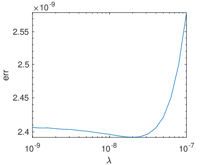
According to the convergence analysis studied in Theorem 4.3, there are three factors that affect the accuracy of our algorithm, i.e., mesh size of FEM basis, regularization factor, and approximation property of the POD basis functions. As such, we set up three experiments when recovering the letter ’A’. Under each experiment, we generate set of observation ’s and solve the optimization with the pre-computed POD basis functions. The standard derivation of the noise is still . It corresponds to a noise level. We compute the mean of the error in each set of parameters and show them in Figure 3.
Dependence on the mesh size
In Figure 3(a) we verify that given when the mesh size of the FEM basis functions goes down, the error of will first decrease and then converged to a limit that is greater than zero. In the first stage, the order of convergence against mesh size is . The limit in the second stage depends on and the dependence is non-monotone. The number of POD basis functions does not change remarkably (also see in the previous example that compares the POD method with FEM) under different mesh sizes. Along with the monotonic decreasing of the error against , it indicates all sets of POD basis functions all approximate some fixed continuous function space.
Dependence on the regularization factor
To further investigate the limiting error, in 3(b), we keep fixed and use different regularization factor ’s. We find that the optimal for with the noise level is between and . The error is a V-shape function near the optimal .
Dependence on the number of POD basis functions
The last experiment is to study how the number of POD basis functions affects the error. In 3(c), we show the mean square error with sets of random generated observation. The error goes down as we increase the number of POD basis functions. The fitted slope in the loglog plot is , which indicates the errors exponentially decay with a coefficient . The p-value for the fitted slope is smaller than .


Iterative algorithm for finding the optimal
As analyzed in Eq.(2.7), the optimal relies on . While in the setting of inverse problems, the norm of input is unknown. A natural choice is to find the optimal by using a fixed-point iteration. To be precise, we start from an initial guess like and solve for with the POD basis functions. After solving the -th step, we update as,
| (5.1) |
We will stop the iteration of until converges. As shown in Figure 4 such iterative algorithms, with either POD or FEM basis, finds the correct scale of with a similar pattern. It implies that the POD method captures the whole solution subspace with given known source function and is robust in iteration. To be noted, in Eq.(2.7), constant is not so the fixed-point iteration Eq.(5.1) only finds the correct scale of comparing with Figure 3(b), in which the error due to is computed with the knowledge of the ground truth solution .


5.2 Recovering Moving Circles
In addition to letter examples, we also applied the POD method to recover a ball pattern that moves on some given trajectories in two-dimensional space. Similar to recovering letters, we construct the POD basis functions from snapshots that are generated by solving forward problems with classic FEM, where the mesh size and time step . is set to be and which corresponds to a noise level.
Moving along a horizontal line
In such case, the source term is given by indicator function of set . When constructing the POD basis functions, we use values of that are equally distributed between interval including two terminal points. basis functions are extracted for accuracy calculated by eigenvalues. In 5 we use the constructed basis on detecting circles with the same size. We find that the performance of the POD method is still acceptable even the centers of the circle do not coincide with the ones when we construct the POD basis functions.
Moving along a ring
In addition, as shown in 6 we recover the same pattern whose center are on a circle. To be specific, the source term is given by indicator function of set . basis are extracted for accuracy. Even with a higher DOF, the POD method still yields acceleration comparing with FEM ( seconds vs seconds).


6 Conclusion
We have developed a data-driven and model-based approach for solving parabolic inverse source problems. The key idea is to exploit (model-based) and construct (data-based) the intrinsic approximate low-dimensional structure of the underlying parabolic PDEs that consists of two components – a training component that constructs a small number of POD basis functions to achieve significant dimension reduction in the solution space, and a fast algorithm that computes the optimization problem in inverse source problem by using the constructed POD basis functions. Hence, we achieve an effective data and model-based approach for the inverse source problems and overcome the typical computational bottleneck of FEM in solving such problems.
Under a weak assumption on the regularity of the solution, we provide the convergence analysis of our POD algorithm in solving the forward parabolic PDEs and thus obtain the error estimate of the POD algorithm for the parabolic inverse source problems. Finally, we carried out numerical experiments to demonstrate the accuracy and efficiency of the proposed method. Through numerical results, we found that our POD algorithm yields as good approximations as the reference solution obtained by the FEM. But our algorithm can be much cheaper. We expect an even better performance of efficiency can be obtained in 3D problems, which is one of our future topics. We also studied other issues of the POD algorithm, such as the dependence of the error on the mesh size, on the regularization parameter in the least-squares regularized minimization problems, and on the number of POD basis functions.
Acknowledgement
The research of W. Zhang is supported by the National Natural Science Foundation of China No. 11901282 and the Shenzhen Sci-Tech Fund No. RCBS20200714114941241. The research of Z. Zhang is supported by Hong Kong RGC grant projects 17300318 and 17307921, National Natural Science Foundation of China No. 12171406, Seed Funding Programme for Basic Research (HKU), and Basic Research Programme (JCYJ20180307151603959) of The Science, Technology and Innovation Commission of Shenzhen Municipality.
References
- [1] V. Akçelik, G. Biros, A. Draganescu, J. Hill, O. Ghattas, and B. Waanders. Dynamic data-driven inversion for terascale simulations: real-time identification of airborne contaminants. In SC’05: Proceedings of the 2005 ACM/IEEE Conference on Supercomputing, pages 43–43. IEEE, 2005.
- [2] A. Alla and M. Falcone. A time-adaptive POD method for optimal control problems. IFAC Proceedings Volumes, 46(26):245–250, 2013.
- [3] P. Benner, S. Gugercin, and K. Willcox. A survey of projection-based model reduction methods for parametric dynamical systems. SIAM Review, 57(4):483–531, 2015.
- [4] P. Benner, S. Gugercin, and K. Willcox. A survey of projection-based model reduction methods for parametric dynamical systems. SIAM Review, 57(4):483–531, 2015.
- [5] G. Berkooz, P. Holmes, and J. Lumley. The proper orthogonal decomposition in the analysis of turbulent flows. Annual review of fluid mechanics, 25(1):539–575, 1993.
- [6] Z. Chen, R. Tuo, and W. Zhang. Stochastic convergence of a nonconforming finite element method for the thin plate spline smoother for observational data. SIAM Journal on Numerical Analysis, 56(2):635–659, 2018.
- [7] Z. Chen, W. Zhang, and J. Zou. Stochastic convergence of regularized solutions and their finite element approximations to inverse source problems. arXiv:2104.02352, 2021.
- [8] Jin Cheng and Jijun Liu. An inverse source problem for parabolic equations with local measurements. Applied Mathematics Letters, 103:106213, 2020.
- [9] Wei Cheng, Ling-Ling Zhao, and Chu-Li Fu. Source term identification for an axisymmetric inverse heat conduction problem. Computers & Mathematics with Applications, 59(1):142–148, 2010.
- [10] S. D’haeyer, B. Johansson, and M. Slodička. Reconstruction of a spacewise-dependent heat source in a time-dependent heat diffusion process. IMA Journal of Applied Mathematics, 79(1):33–53, 2014.
- [11] A. El Badia, A. El Hajj, M. Jazar, and H. Moustafa. Lipschitz stability estimates for an inverse source problem in an elliptic equation from interior measurements. Applicable Analysis, 95(9):1873–1890, 2016.
- [12] A. El Badia, T. Ha Duong, and F. Moutazaim. Numerical solution for the identification of source terms from boundary measurements. Inverse Problems in Engineering, 8(4):345–364, 2000.
- [13] A. El Badia and T. Nara. An inverse source problem for Helmholtz’s equation from the Cauchy data with a single wave number. Inverse Problems, 27(10):105001, 2011.
- [14] G. Garcia, A. Osses, and M. Tapia. A heat source reconstruction formula from single internal measurements using a family of null controls. Journal of Inverse and Ill-posed Problems, 21(6):755–779, 2013.
- [15] S. Gorelick, B. Evans, and I. Remson. Identifying sources of groundwater pollution: an optimization approach. Water Resources Research, 19(3):779–790, 1983.
- [16] H. Gu, J. Xin, and Z. Zhang. Error estimates for a POD method for solving viscous G-equations in incompressible cellular flows. SIAM Journal on Scientific Computing, 43(1):A636–A662, 2021.
- [17] J. Hadamard. Lectures on Cauchy’s problem in linear partial differential equations. Courier Corporation, 2003.
- [18] J. Hesthaven, G. Rozza, and B. Stamm. Certified reduced basis methods for parametrized partial differential equations. Springer, 2016.
- [19] P. Holmes, J. Lumley, and G. Berkooz. Turbulence, coherent structures, dynamical systems and symmetry. Cambridge University Press, 1998.
- [20] V. Isakov. Inverse problems for partial differential equations, volume 127. Springer, 2006.
- [21] V. Isakov, S. Leung, and J. Qian. A three-dimensional inverse gravimetry problem for ice with snow caps. Inverse Problems & Imaging, 7(2):523, 2013.
- [22] T. Johansson and D. Lesnic. Determination of a spacewise dependent heat source. Journal of computational and Applied Mathematics, 209(1):66–80, 2007.
- [23] K. Kunisch and S. Volkwein. Galerkin proper orthogonal decomposition methods for parabolic problems. Numerische Mathematik, 90(1):117–148, 2001.
- [24] K. Kunisch, S. Volkwein, and L. Xie. HJB-POD-based feedback design for the optimal control of evolution problems. SIAM Journal on Applied Dynamical Systems, 3(4):701–722, 2004.
- [25] X. Liu. Identification of indoor airborne contaminant sources with probability-based inverse modeling methods. Boulder, CO: PhD dissertation. University of Colorado at Boulder, 2008.
- [26] X. Liu and Z. Zhai. Inverse modeling methods for indoor airborne pollutant tracking: literature review and fundamentals. Indoor air, 17(6):419–438, 2007.
- [27] P. Nelson and S. Yoon. Estimation of acoustic source strength by inverse methods: Part i, conditioning of the inverse problem. Journal of sound and vibration, 233(4):639–664, 2000.
- [28] G. Nunnari, A. Nucifora, and C. Randieri. The application of neural techniques to the modelling of time-series of atmospheric pollution data. Ecological Modelling, 111(2-3):187–205, 1998.
- [29] A. Quarteroni, A. Manzoni, and F. Negri. Reduced basis methods for partial differential equations: an introduction, volume 92. Springer, 2015.
- [30] M. Renardy and R. Rogers. An introduction to partial differential equations, volume 13. Springer Science & Business Media, 2006.
- [31] L. Sirovich. Turbulence and the dynamics of coherent structures. I. Coherent structures. Quarterly of applied mathematics, 45(3):561–571, 1987.
- [32] L. Sirovich. Turbulence and the dynamics of coherent structures. I. Coherent structures. Quarterly of applied mathematics, 45(3):561–571, 1987.
- [33] V. Thomée. The finite element method for parabolic problems. In Mathematical Theory of Finite and Boundary Element Methods, pages 135–218. Springer, 1990.
- [34] S. Volkwein. Proper orthogonal decomposition: Theory and reduced-order modelling. Lecture Notes, University of Konstanz, 4(4), 2013.
- [35] J. Wong and P. Yuan. A FE-based algorithm for the inverse natural convection problem. International Journal for numerical methods in fluids, 68(1):48–82, 2012.