Fitting three-dimensional Laguerre tessellations by hierarchical marked point process models
Abstract
We present a general statistical methodology for analysing a Laguerre tessellation data set viewed as a realization of a marked point process model. In the first step, for the point, we use a nested sequence of multiscale processes which constitute a flexible parametric class of pairwise interaction point process models. In the second step, for the marks/radii conditioned on the points, we consider various exponential family models where the canonical sufficient statistic is based on tessellation characteristics. For each step, parameter estimation based on maximum pseudolikelihood methods is tractable. For model selection, we consider maximized log pseudolikelihood functions for models of the radii conditioned on the points. Model checking is performed using global envelopes and corresponding tests in both steps and moreover by comparing observed and simulated tessellation characteristics in the second step. We apply our methodology for a 3D Laguerre tessellation data set representing the microstructure of a polycrystalline metallic material, where simulations under a fitted model may substitute expensive laboratory experiments.
Keywords:
exponential family model , global envelope test , multiscale process , polycrystalline microstructure , pseudolikelihood2010 MSC
60G551 Introduction
This paper develops new statistical methodology for analysing Laguerre tessellation data sets, where we illustrate how the methodology applies for an example of a 3D Laguerre tessellation data set representing a polycrystalline material.
1.1 Some background and motivation
In brief, a 3D Laguerre tessellation (also called a power diagram or a generalised Voronoi tessellation) is a flexible way of modelling a subdivision of 3D space (see Section 2 for the details). In practice the tessellation is described by a data set where is a finite point pattern and is an associated vector of positive numbers called marks, and we identify by the marked point pattern (see again Section 2 for the details). Such data sets appear in various contexts of material science. For example, in 3D X-ray diffraction microscopy of polycrystalline materials the volumes and centroids of grains are obtained, and representation of such measurements by a 3D Laguerre tessellation can be produced by various optimization methods [Lyckegaard et al. 2011, Spettl et al. 2016, Quey and Renversade 2018, Kuhn et al. 2020]. It is then useful to develop stochastic models for the tessellation since simulations can to some extent substitute expensive laboratory experiments. However, only a few papers [Spettl et al. 2015, Seitl et al. 2021, including] have been dealing with statistical methodology in the context of polycrystalline materials.
Inference for statistical models of Laguerre tessellation data sets is a difficult task unless follows a simple model such as a (marked) Poisson process which in practice is rarely a reasonable assumption. Often the points in exhibit regularity and different marked point process models for have been suggested: simple random models for packings of hard balls [Chiu et al. 2013] obtained by iterative procedures such as random sequential adsorption [Lautensack 2008, with applications to foam structures] or variants of collective-rearrangement algorithms [Spettl et al. 2015, with application to a polycrystalline microstructure]; and inspired by the work in Dereudre and Lavancier 2011 on Gibbsian models for 2D Voronoi tessellations, Seitl et al. 2021 introduced Gibbsian models for random 3D Laguerre tessellations. These Gibbs models were first thought to be tempting to use because they may incorporate properties of the Laguerre tessellation and interaction between its cells. However, the models are complicated to use for statistical inference and they are time-consuming to simulate.
1.2 Our contribution
In this paper we introduce hierarchical statistical models consisting of first a parametric Gibbs point process model for and second a parametric model for conditioned on . Specifically, we use in the first case a nested sequence of flexible pairwise interaction points processes called multiscale processes [Penttinen 1984] and in the second case various exponential family models where the canonical sufficient statistic is based on tessellation characteristics such as surface area or volume of cells or absolute difference in volumes of neighbouring cells. Apart from reducing the dimension from 4 (when viewing as a 4-dimensional point pattern) to 3 (when considering ), an advantage is that we specify two much simpler cases of models with parameters which do not depend on each other. Hence we can separate between how to simulate and estimate unknown parameters for and , respectively. The parameters are simply estimated by maximum pseudolikelihood methods and well-known MCMC algorithms are used for simulations. Thereby estimation and simulation become much faster than in Seitl et al. 2021 when fitting specific models given in Section 4 and used for analysing the data from Section 3 in Section 5.
A further advantage is that the model construction makes it possible to develop a rather straightforward model selection procedure: For , the procedure starts with the simplest case of a Poisson process and continues with constructing more and more complex multiscale processes until a satisfactory fit is obtained when considering global envelopes and tests [Myllymäki et al. 2017] based on various functional summary statistics. For conditioned on , more and more complex exponential models are developed, where we demonstrate how to compare fitted models of the same dimension by considering maximized log pseudolikelihood functions. Further, we evaluate selected fitted models by comparing moment properties of tessellation characteristics under simulations from the model with empirical moments, by considering plots of global envelopes, and by evaluating values of global envelope tests. This comparison is not only done by looking at those tessellation characteristics used for specifying the canonical sufficient statistic of the exponential model but also for various other tessellation characteristics. To the best of our knowledge, this is the first time that such a model selection procedure has been used when analysing polycrystalline materials, cf. Šedivý et al. 2018 and the references therein.
For the computations of Laguerre tessellations, we use the C++ library Voro++ [Rycroft 2009]. This open source library enables computation of single Laguerre cells which is an advantage for the estimation and MCMC simulation procedures we use. For the calculation of functional summary statistics (specifically , and ), we use the R-package spatstat [Baddeley et al. 2015], and for global envelopes and corresponding -values we use the R-package GET [Myllymäki and Mrkvička 2019]. We implemented a code for pseudolikelihood estimation and the MCMC algorithms used for simulation of the point process models and the models for the radii given the points. This code is available at https://github.com/VigoFierry/Lag_mod.
The paper is organised as follows. Section 2 provides details on Laguerre tessellation data sets. Section 3 describes a particular data set which in later sections is used to illustrate our statistical methodology. Section 4 specifies our hierarchical model construction and discusses how we used maximum pseudolikelihood estimation and simulated under fitted models for and . Section 5 details our model selection procedure and applies it on the Laguerre tessellation data set from Section 3. Finally, Section 6 contains concluding remarks. The paper is accompanied by supplementary material available in appendices A-E in this preprint.
2 Laguerre tessellation data sets
A Laguerre tessellation is defined as follows. Consider a marked point pattern where each is a spatial location with an associated mark and the index set is finite or countable. Define the corresponding point configuration and the associated (possibly infinite) vector of marks (using some arbitrary ordering of ). Interpret as a closed ball with center and radius , and define the power distance from a point to this ball by
where denotes Euclidean distance. Assuming that exists for every , the Laguerre cell with generator is
and the Laguerre tessellation generated by is the collection of all non-empty cells .
Notice that and are in one-to-one correspondence. We use this identification without any mentioning in the following. But it should be kept in mind when we abuse terminology by calling a marked point pattern, and when we abuse notation and write e.g. (which means that for some ).
We refer to Lautensack and Zuyev 2008 and the references therein for detailed studies of deterministic and random Laguerre tessellations. The reason why Laguerre tessellations are so useful for modelling purposes may be explained by a fundamental result due to Aurenhammer 1987 and extended by Lautensack and Zuyev 2008 to infinite cases: any 3D (or higher-dimensional) normal tessellation with convex cells is a Laguerre tessellation.
In Section 3 and later sections we consider the following setting. Let be a rectangular parallelepiped and a finite marked point pattern such that . Define a periodic extension of which is in accordance to , i.e., the infinite marked point pattern
| (1) |
where is the 3D integer lattice. Note that . Then we consider the Laguerre tessellation generated by and keep only those Laguerre cells which are non-empty and have . Let be the number of such cells and be the marked point pattern specifying the generators of these cells. Then is the Laguerre tessellation data set used for our statistical analysis.
This construction of is one way of how Laguerre tessellation data sets may be produced, and we will consider as a realisation of a finite marked point process [Chiu et al. 2013, for background material on marked point processes, see e.g.]. Note that the statistical methodology introduced in this paper can immediately be extended to other settings with a finite marked point pattern data set representing a Laguerre tessellation.
3 Application example
The Laguerre tessellation data set used throughout the text to illustrate our statistical methodology is related to a study in Sedmák et al. 2016 of a polycrystalline microstructure of a nickel titanium alloy. Using a notation as in Section 2, we deal with a finite marked point pattern extracted from a larger data set collected in Petrich et al. 2019 by the so-called cross-entropy method applied to 3D X-ray diffraction measurements. Specifically, consists of the 2009 points which are contained in a 3D rectangular observation window of size (the units being micrometers), where is a cut-off from the entire material specimen. Some of the cells in the Laguerre tessellation generated by are unbounded and hence not contained in the material specimen. To account for this and for computational reasons (i.e., the use of Voro++), we choose to apply a periodic extension thereby obtaining our Laguerre tessellation data set , cf. Section 2. Here , so by applying the periodic extension at most 44 cells are ‘lost’.
The left panel in Figure 1 below depicts together with and A and B show images of the observed Laguerre tessellation together with plots of the projections of onto the , and planes, respectively. None of these indicate spatial inhomogeneity of . So considering the periodic extension (defined as in (1) but with replaced by ), we find it reasonable to assume that the distribution underlying is invariant under translations in 3D space. Equivalently, we assume that the distribution underlying is invariant under shifts when is wrapped on a 3D torus. The right panel in Figure 1 shows the balls defined by . This indicates that the distribution underlying the radii conditioned on can be assumed to be homogeneous, i.e., we have invariance in this conditional distribution when making shifts of on the torus. This assumption is further supported by plots in B showing the radii distributions corresponding to a subdivision of into sets of equal size and shape. Moreover, Figure 2 below shows a histogram of the radii together with a kernel density estimate and the density of a beta distribution fitted by maximum pseuodolikelihood estimation as discussed later in Sections 4 and 5.

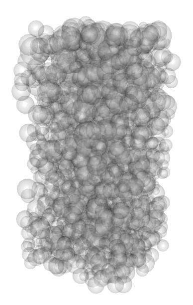
Figure 3 shows estimated/empirical functional summary statistics , and for the point pattern where we used the R-package spatstat [Baddeley et al. 2015] for the calculations. For definitions and interpretations of these empirical functions using edge correction factors, see e.g. Baddeley et al. 2015 (for we used Ripley’s isotropic edge correction factor and for and we used Kaplan-Meier edge correction factors). Figure 3 also shows a concatenated 95%-global envelope/confidence region (the grey region) under a homogeneous Poisson process (with the intensity estimated by divided by the volume of ), meaning that under this Poisson process all three empirical functions are expected to be within the envelope with probability 0.95. The envelopes were obtained using the R-package GET [Myllymäki and Mrkvička 2019] with 1999 simulations of the Poisson process (increasing this to 9999 simulations did not change the results). The plots show that the empirical functions are often outside the envelope, and the corresponding -value obtained by the global area rank envelope test [Myllymäki et al. 2017] is below 0.1% [Myllymäki and Mrkvička 2020, there are several possible choices of making an envelope test, but the area rank envelope test is recommended in]. The way the functions based on the data differ from the envelope indicates regularity in the point pattern .


Figure 4 depicts histograms of some cell characteristics: volume of a cell (abbreviated as ‘vol’); number of faces in a cell (‘nof’); sphericity of a cell (‘spher’) as defined by
where ‘surf’ means surface area of a cell; and absolute difference in volume ‘dvol’ for two neighbouring cells (i.e., they share a face). Note that with the value 1 corresponding to a sphere. Figure 4 shows that many cells are small, the distribution of nof is rather symmetric and ranges from 4 (the smallest possible value) to 35, many cells are rather spherical and many pairs of neighbouring cells have a range of differences in cell sizes in the same order as the cell size itself.


The upper right triangle in Table 1 shows the empirical correlations for the cell characteristics vol, surf, nof and spher together with a new cell characteristic, namely total edge length in a cell (‘tel’). The lower left triangle in the table shows the empirical correlations for dvol and three other face characteristics: area of a face (‘farea’), perimeter of a face (‘fper’) and number of edges in a face (‘fnoe’). We see that all correlations are high except for dvol which is nearly uncorrelated to any other face characteristic. In particular vol, surf and tel are highly correlated, and farea and fper are highly correlated (correlations ).
| vol | 0.971 | 0.938 | 0.841 | 0.680 |
| farea | surf | 0.974 | 0.874 | 0.737 |
| 0.923 | fper | tel | 0.941 | 0.793 |
| 0.751 | 0.751 | fnoe | nof | 0.754 |
| 0.074 | 0.062 | 0.025 | dvol | spher |
To see if there is dependence between and , we follow Stoyan et al. 2021 and consider the empirical mark correlation function. We perform a permutation test based on the global area rank envelope test, permuting 1000 times the marks/radii when is fixed and calculating the empirical mark correlation function each time. Figure 5 shows the function based on the data: it falls outside the 95%-global envelope on two intervals, and the corresponding -value obtained by the global area rank envelope test is 1.4%, so we reject the null hypothesis of independence between and .

4 Hierarchical model
This section details the two steps of our hierarchical model construction which was briefly discussed in Section 1. To avoid confusion, we reserve the notation for the data and use the notation when we consider arguments of densities where is a finite point configuration and are associated marks (if then is the empty point configuration and can be ignored).
4.1 Point process models for
When modelling the point pattern data set as a realization of a spatial point process on , we refer to Møller and Waagepetersen 2004 for background material on spatial point process models. In accordance to our observations in Section 3, we assume that the distribution of is invariant under shifts when wrapping on a 3D torus, and a model for should exhibit regularity. Pairwise interaction point processes constitute a flexible class model for regularity. Recall that is a pairwise interaction point process on with homogeneous interaction functions (with respect to shifts on wrapped on a 3D torus) if its distribution is given by a density with respect to the unit rate Poisson process on , where the density is of the form
for and every point configuration . Here is a parameter, denotes shortest distance on wrapped on a 3D torus, is a so-called interaction function and is a normalising constant which depends on and . In order to obtain a well-defined density, a further condition on the interaction function is needed; it suffices to assume that in which case .
As a parametric approximation of such a pairwise interaction point process we consider a multiscale process [Penttinen 1984]: for , let denote the model class given by densities of the form
| (2) |
where , , , and are unknown parameters. Here we have omitted the normalising constant (which depends on all parameters), denotes the indicator function and we set and . If we interpret the right hand side in (2) as . Note that is just a homogeneous Poisson process on with intensity and is just a Strauss process.
Simulation under the Poisson model is well-known (see e.g. Møller and Waagepetersen 2004) and for simulation of the models , , we used the birth-death-move Metropolis-Hastings algorithm [Geyer and Møller 1994, Møller and Waagepetersen 2004].
4.2 Exponential tessellation models for given
When modelling the observed radii as a realisation of an -dimensional vector, we condition on and consider a conditional probability density function (pdf) on . More precisely we assume is a random vector (of random length) which conditioned on has a conditional pdf which is zero whenever for some . Furthermore, in order to work with a well-defined conditional pdf in (3) below we assume a mark space so that if ; this is in accordance to our data, where and .
We now give a general exponential family form of the conditional pdf where is the dimension, denotes the canonical parameter and the canonical sufficient statistic: for ,
| (3) |
The idea is to let each depend on either the radii, or tessellation characteristics of the cells with or interactions between these cells (here is defined in a similar way as , i.e., in the right hand side of (1) is replaced by ). Specifically, in Section 5 we consider the following cases (a)–(e), using similar abbreviations as in Section 3, for short writing for and considering in (b)–(d) a sum over the cells , , and in (e) a sum over all unordered pairs of cells sharing a face:
- (a)
including both and (with ) somehow corresponds to a scaled beta distribution for the radii if no other terms are included in (3) – ‘somehow’ because it is not exactly a beta distribution since if for some ;
- (b)
is twice the total number of faces;
- (c)
is twice the total surface area of faces;
- (d)
is the sum of squared volumes of cells;
- (e)
is the sum of difference in volumes of two cells which share a face.
The density in (3) is then well-defined for all provided in case of (a) we have and ; this follows since the mark space is bounded. Moreover, for simulation under (3) we use a Metropolis within Gibbs algorithm where we alternate between updating from the conditional densities
| (4) |
using a Metropolis algorithm with a normal proposal.
4.3 Estimation
We assume that the unknown parameter in (3) varies independently of the parameters in (2). Then parameter estimation can be done in two steps and the results will not depend on each other.
To avoid calculating the intractable normalising constants appearing in (2) and (3), we use maximum pseudolikelihood methods [Besag 1974, Besag 1977, Besag et al. 1982] in both cases where a few remarks are in order: For the definition of pseudolikelihood function in connection to (2), we refer to Jensen and Møller 1991; see also D. For fixed , (2) is an exponential family model with canonical parameter and so the log pseudolikelihood function is a concave function of [Jensen and Møller 1991] and we can find a partial maximum pseudolikelihood estimate (MPLE) of using the Newton-Raphson algorithm. Hence we obtain a profile log pseudolikelihood which is maximised with respect to defined over a -dimensional grid, thereby providing the final MPLE. Furthermore, when considering (3) the pseudolikelihood for is defined by the product of the conditional densities of each given the with , cf. (4). Since (3) is also an exponential family, the log pseudolikelihood is concave and then again Newton-Raphson can be used for finding the MPLE. Finally, we calculate various integrals which appear in the pseudolikelihoods (in case of (2), see Jensen and Møller 1991; in case of (3), we consider the integral of the right hand side of (4) with respect to ) by numerical methods.
5 Model selection and final joint model
This section details the model selection procedure briefly described in Section 1.2 and which leads to our final joint model for and . The classical goodness of fit procedures are based on measures given by maximizing likelihood functions and accounting for model complexity by including a penalty in terms of the number of parameters (e.g. AIC and BIC criteria). In Šedivý et al. 2018 the Vapnik-Chervonenkis theory is used instead and a criterion based on residual sum of squares is developed for partially ordered sets of deterministic tessellation models. Since we deal with stochastic tessellation models but our likelihood functions are intractable to maximize, we present another approach that corresponds to modern trends in spatial statistics. It is based on how well geometrical tessellation characteristics are described when comparing fitted models, where we account for mutual correlations among the characteristics and we consider the maximum of pseudolikelihood functions when comparing models with the same number of parameters.
5.1 The fitted model for
For the point pattern and , we select the first model which provides a satisfactory fit when considering global envelopes and global area rank envelope test in the same way as in Section 3. As noticed in Section 3, the Poisson model is not providing a satisfactory fit and as discussed in C this is also the case for the Strauss model . The first model which is not significant at level 5% is : Figure 6 shows that the empirical functional summary statistics are within the 95%-global envelope produced in a similar way as in Figure 3 but using simulations under the fitted multiscale process with . The corresponding -value obtained by the global area rank envelope test is , and the maximum pseudolikelihood estimates (see Section 4.3) are , , , and .


5.2 The fitted model for conditioned on
Now, having fitted the model for it remains to obtain a model for conditioned on where we use a model selection procedure as follows. We consider a list of tessellation characteristics
| (5) |
when creating and evaluating more and more complex models as given by (3) and (a)–(e) in Section 4.2. When comparing fitted models of the same dimension , we select the one with the highest value of the maximized log pseudolikelihood function. The selected model is then evaluated by a global area rank envelope test based on kernel smoothed densities of the empirical distributions for the six tessellation characteristics in , using simulations of the joint model for and . Here we concatenate the six densities and use the R-package GET [Myllymäki and Mrkvička 2019], and we simulate from the joint model rather than from the conditional model of given , since our aim is to replace expensive laboratory experiments with simulations from the joint model. Therefore, in Table 2, we also evaluate our fitted models by comparing empirical (column ‘data’) and simulated means and standard deviations of the tessellation characteristics in , using 100 simulations of first and second under the different fitted models of conditioned on . The table also shows the (signed) difference between the empirical and the simulated values divided by the empirical values (the values given in percentages) – we refer to such a value as a deviation.
First, we consider the empirical distribution of the radii: As the histogram in Figure 2 looks like a beta distribution, we first propose in (3) only to include the terms in (a) so that , and – we refer to this model as ‘beta’. The column ‘beta’ in Table 2 shows that except for dvol the means match the data well, and the deviations of standard deviations vary by to percent. However, the fitted ‘beta’ model was highly significant when evaluated by the global area rank envelope test.
| models | data | ||||
|---|---|---|---|---|---|
| beta | |||||
| nof | mean | 14.82 | 14.87 | 14.95 | 14.98 |
| -1% | -1% | -1% | |||
| sd | 5.58 | 5.38 | 5.20 | 4.92 | |
| +13% | +9% | +6% | |||
| vol | mean | 70.65 | 70.65 | 70.65 | 69.21 |
| +2% | +2% | +2% | |||
| sd | 65.65 | 63.42 | 62.01 | 58.89 | |
| +12% | +8% | +5% | |||
| surf | mean | 91.14 | 91.53 | 93.58 | 92.46 |
| -1% | -1% | +1% | |||
| sd | 57.26 | 54.07 | 51.50 | 47.86 | |
| +20% | +13% | +8% | |||
| tel | mean | 66.16 | 66.12 | 67.69 | 67.92 |
| -3% | -3% | -1% | |||
| sd | 31.99 | 30.86 | 29.52 | 27.38 | |
| +17% | +13% | +8% | |||
| spher | mean | 0.76 | 0.76 | 0.77 | 0.78 |
| -3% | -3% | -1% | |||
| sd | 0.11 | 0.10 | 0.10 | 0.087 | |
| +24% | +19% | +16% | |||
| dvol | mean | 79.87 | 73.72 | 69.82 | 68.89 |
| +16% | +7% | +1% | |||
| sd | 72.75 | 68.57 | 62.78 | 65.04 | |
| +12% | +5% | -4% |
Second, we expand the model by including one of the terms , , or so that . Here, we do not include , since this is a constant; or , since the correlation coefficient between vol and tel for each cell is close to 1; or , since by definition spher is given by vol and surf for each cell. Table 3 shows that the model with has the largest maximized log pseudolikelihood function. For this model, comparing the columns ‘beta’ and ‘beta+dvol’ in Table 2 we obtain now better results for dvol. Moreover, all standard deviations are now reduced, and the -value based on global area rank envelope test is 9.8%.
Third, we investigate the effect of expanding the model ‘beta’ with any two of the four terms , , and so that . Table 3 shows that ‘beta+nof+dvol’ provides the best fit according to the maximized log pseudolikelihood function. For this model, the -value based on global area rank envelope test is 10.6% which is slightly larger than the -value of 9.8% for the model ‘beta+dvol’. Table 2 shows an improvement for both the mean values and the standard deviations when comparing ‘beta+nof+dvol’ with ‘beta+dvol’. Figure 7 shows empirical kernel estimates of the densities for the six characteristics in together with a -global envelope obtained when concatenating all six empirical densities. The empirical functions are completely covered by the envelope. Moreover, the maximum pseudolikehood estimates are , , and . Thus under this fitted model realisations become more likely as the total number of faces decreases or the sum of differences in volumes between neighbouring cells increases (when all other terms in (3) are fixed).
In a similar way, we also tried fitting models without including the terms in (a), thereby obtaining ‘nof+surf+dvol’ as the final model for and where the -value is 7.7%. A plot similar to Figure 7 but for the fitted ‘nof+surf+dvol’ model is given in E.
| model | PL |
|---|---|
| -2532.45 | |
| -2866.39 | |
| -2594.72 | |
| -2483.98 | |
| -2468.76 | |
| -2513.89 | |
| -2823.71 | |
| -2714.10 | |
| -2498.58 | |
| -2465.12 | |
| -2477.63 |

6 Concluding remarks
Our hierarchical model construction for Laguerre tessellation data sets, using a Gibbs model for the points and a conditional model for the radii given the points, may be useful in several other contexts, including 2D cases. As compared to the use of Gibbs models in Dereudre and Lavancier 2011 and Seitl et al. 2021, our hierarchical approach is less time demanding: To simulate a vast number of standard point process models is a routine task which is not too much time demanding. The more exhaustive part is to simulate the radii since Laguerre cells have to be recomputed, but still in comparison with Seitl et al. 2021 it becomes faster in our case since we condition on the points.
For the Gibbs point process model, we considered multiscale models which approximate the class of pairwise interaction point processes and lead to a natural model selection procedure by considering an increasing number of interaction parameters. We might consider point process models with higher order interactions such as Geyer’s triplet interaction process [Geyer 1999] or the area interaction process involving interactions of all orders [Baddeley and Van Lieshout 1995]. However, the computational complexity increases with more complex models.
For the conditional distribution of radii given points, we have demonstrated the usefulness of exponential family models with a canonical sufficient statistic based on tessellation characteristics. As there are several possibilities for selecting tessellation characteristics and there is no natural ordering (as there is in the case of the multiscale model), a model selection procedure is less straightforward. However, we demonstrated how to compare fitted models of the same dimension by considering maximized log pseudolikelihood functions and how to evaluate selected fitted models by partly comparing moment properties of tessellation characteristics under simulations from the model with empirical moments and partly by considering plots of global envelopes and by evaluating their corresponding -values.
When calculating pseudolikelihood functions, various integrals have to be evaluated, cf. Section 4.3. We used simple grid-based approximation methods for both the pseudolikelihood based on the points and that based on the radii given the points. A small simulation study indicated that this may cause some bias in the MPLEs (also for MPLEs of the Gibbs models in Dereudre and Lavancier 2011 and Seitl et al. 2021 some bias appeared). Baddeley and Turner 2014 noticed that bias of MPLEs for spatial point process models usually does not reflect weaknesses of the MPLE method, but is probably due to the effects of discretization of the observation window. For 2D spatial point process models, efficient numerical methods have been developed [Baddeley and Turner 2014, Baddeley et al. 2014] and spatstat provides useful software, but to the best of our knowledge it remains to make progress for in general 3D point processes and for the special case of our model. We leave this important and huge task for future research.
Acknowledgements
The research was supported by the Czech Science Foundation, project 19-04412S, and by The Danish Council for Independent Research —
Natural Sciences, grant DFF – 7014-00074 ‘Statistics for point processes in space and beyond’. We thank the referees for useful comments and suggestions.
Appendix A Visualization of the observed Laguerre tessellation
In order to visualize the Laguerre tessellation data set described in Section 3, Figure 8 shows four equidistant slices perpendicular to the axis.
Appendix B Homogeneity of points and radii
The key assumption of homogeneity of and conditioned on is investigated in this section. Figure 9 depicts together with the observation window and the projections of onto , and planes. The figure indicates spatial homogeneity of . In Figure 10, the left panel shows a kernel density estimate of the radii distribution and, for comparison purposes, the right panel shows eight kernel density estimates of the radii distributions corresponding to a subdivision of into the subsets obtained by dividing the three sides of the rectangular region into half sides. For the number of points per subset, the mean is , the minimum is and the maximum is . The similarity of the eight density estimates is in accordance with the assumption that the distribution of conditioned on is homogeneous.

.
Appendix C Strauss process
Figure 11 shows three empirical functional summary statistics together with -global envelopes obtained by simulations under the Strauss process model (the multiscale process with ) fitted by maximum pseudolikelihood. The corresponding -value obtained by the global area rank envelope test is .


Appendix D Pseudolikelihood functions
D.1 Pseudolikelihood for the points
As in the paper, consider a point process with a given realization in the observation window and modelled by a parametric density (with respect to the unit rate Poisson process) where is an unknown real parameter vector. Assume is hereditary, i.e., for we have whenever . Then the pseudolikelihood function for the points is
where is the Papangelou conditional intensity (setting ). Denoting the natural logarithm by , the log pseudolikelihood function in the case of the multiscale process (see (2) with ) becomes
where and .
D.2 Pseudolikelihood for the radii given the points
Denoting the conditional density (3) by , the pseudolikelihood function for the radii given the points is
where . Assume that is feasible, i.e., all Laguerre cells are nonempty; we denote this property by . Then the log pseudolikelihood function for the radii distribution given the points is
where .
Appendix E A model for the radii given the points where the ‘beta’ term does not appear
In order to see the effect of omitting the ‘beta’ term in the density (3) for the radii conditioned on the points, we fitted the model ‘nofsurfdvol’ corresponding to in (3). Since this is a three-dimensional model, we compare with the results for the fitted three-dimensional model ‘beta+dvol’ in the paper.
Figure 12 shows empirical kernel estimates of the densities for the six characteristics in (see (5)) together with a -global envelope obtained when concatenating all six empirical densities and using the R-package GET with simulations of the fitted joint model for and . The plots show that the functions based on the data are completely covered by the envelope. Moreover, the corresponding -value obtained by the global area rank envelope test is 7.7%, which is less than the -value 9.8% obtained for the fitted ‘beta+dvol’ model. Finally, the maximum pseudolikehood estimates are , and , and the value of the maximized log pseudolikelihood function is , which is smaller than the corresponding value of for the fitted ‘beta+dvol’ model.

References
- Aurenhammer [1987] Aurenhammer, F., 1987. A criterion for the affine equivalence of cell complexes in and convex polyhedra in . Discrete Computational Geometry 2, 49–64.
- Baddeley et al. [2014] Baddeley, A., Coeurjolly, J.F., Rubak, E., Waagepetersen, R., 2014. Logistic regression for spatial Gibbs point processes. Biometrika 101, 377–392.
- Baddeley et al. [2015] Baddeley, A., Rubak, E., Turner, R., 2015. Spatial Point Patterns: Methodology and Applications with R. Chapman & Hall/CRC, Boca Raton.
- Baddeley and Turner [2014] Baddeley, A., Turner, R., 2014. Bias correction for parameter estimates of spatial point process models. Journal of Statistical Computation and Simulation 84, 1621–1643.
- Baddeley and Van Lieshout [1995] Baddeley, A.J., Van Lieshout, M.N.M., 1995. Area-interaction point processes. Annals of the Institute of Statistical Mathematics 47, 601–619.
- Besag [1974] Besag, J.E., 1974. Spatial interaction and the statistical analysis of lattice systems (with discussion). Journal of the Royal Statistical Society Series B 36, 192–236.
- Besag [1977] Besag, J.E., 1977. Some methods of statistical analysis for spatial data. Bulletin of the International Statistical Institute 47, 77–92.
- Besag et al. [1982] Besag, J.E., Milne, R.K., Zachary, S., 1982. Point process limits of lattice processes. Journal of Applied Probability 19, 210–216.
- Chiu et al. [2013] Chiu, S.N., Stoyan, D., Kendall, W.S., Mecke, J., 2013. Stochastic Geometry and Its Applications. John Wiley & Sons, Chichester.
- Dereudre and Lavancier [2011] Dereudre, D., Lavancier, F., 2011. Practical simulation and estimation for Gibbs Delaunay–Voronoi tessellations with geometric hardcore interaction. Computational Statistics & Data Analysis 55, 498–519.
- Geyer [1999] Geyer, C.J., 1999. Likelihood inference for spatial point processes, in: Barndorff-Nielsen, O.E., Kendall, W.S., van Lieshout, M.N.M. (Eds.), Stochastic Geometry: Likelihood and Computation. Chapman & Hall/CRC, Boca Raton, pp. 141–172.
- Geyer and Møller [1994] Geyer, C.J., Møller, J., 1994. Simulation procedures and likelihood inference for spatial point processes. Scandinavian Journal of Statistics 21, 359–373.
- Jensen and Møller [1991] Jensen, J.L., Møller, J., 1991. Pseudolikelihood for exponential family models of spatial point processes. The Annals of Applied Probability 1, 445–461.
- Kuhn et al. [2020] Kuhn, J., Schneider, M., Sonnweber-Ribic, P., Boelke, T., 2020. Fast methods for computing centroidal Laguerre tessellations for prescribed volume fractions with applications to microstructure generation to polycrystalline materials. Computer Methods in Applied Mechanics and Engineering 369, 113–175.
- Lautensack [2008] Lautensack, C., 2008. Fitting three-dimensional Laguerre tessellations to foam structures. Journal of Applied Statistics 35, 985–995.
- Lautensack and Zuyev [2008] Lautensack, C., Zuyev, S., 2008. Random Laguerre tessellations. Advances in Applied Probability 40, 630–650.
- Lyckegaard et al. [2011] Lyckegaard, A., Lauridsen, E., Ludwig, W., Fonda, R., Poulsen, H., 2011. On the use of Laguerre tessellations for representations of 3D grain structures. Advanced Engineering Materials 13, 165–170.
- Møller and Waagepetersen [2004] Møller, J., Waagepetersen, R.P., 2004. Statistical Inference and Simulation for Spatial Point Processes. Chapman & Hall/CRC, Boca Raton.
- Myllymäki and Mrkvička [2019] Myllymäki, M., Mrkvička, T., 2019. GET: Global Envelopes in R. Avaliable at arXiv:1911.06583.
- Myllymäki and Mrkvička [2020] Myllymäki, M., Mrkvička, T., 2020. Comparison of non-parametric global envelopes. Avaliable at arXiv:2008.09650.
- Myllymäki et al. [2017] Myllymäki, M., Mrkvička, T., Seijo, H., Grabarnik, P., Hahn, U., 2017. Global envelope tests for spatial processes. Journal of the Royal Society of Statistics Series B 79, 381–404.
- Penttinen [1984] Penttinen, A., 1984. Modelling Interactions in Spatial Point Patterns: Parameter Estimation by the Maximum Likelihood Method. Number 7 in Jyväskylä Studies in Computer Science, Economics and Statistics, University of Jyväskylä.
- Petrich et al. [2019] Petrich, L., Staněk, J., Wang, M., Westhoff, D., Heller, L., Šittner, P., Krill, III, C., Beneš, V., Schmidt, V., 2019. Reconstruction of grains in polycrystalline materials from incomplete data using Laguerre tessellations. Microscopy and Microanalysis 25, 743–752.
- Quey and Renversade [2018] Quey, R., Renversade, L., 2018. Optimal polyhedral description of 3D polycrystals: Method and application to statistical and synchrotron X-ray diffraction data. Computational Methods in Applied Mechanical Enginering 330, 308–333.
- Rycroft [2009] Rycroft, C.H., 2009. A three-dimensional Voronoi cell library in C++. Chaos 19, 041111.
- Sedmák et al. [2016] Sedmák, P., Pilch, J., Heller, L., Kopeček, J., Wright, J., Sedlák, P., Frost, M., Šittner, P., 2016. Grain-resolved analysis of localized deformation in nickel-titanium wire under tensile load. Science 353, 559–562.
- Seitl et al. [2021] Seitl, F., Petrich, L., Staněk, J., Krill, C.E., Schmidt, V., Beneš, V., 2021. Exploration of Gibbs-Laguerre tessellations for three-dimensional stochastic modeling. Methodology and Computing in Applied Probability, 23, 669–693.
- Spettl et al. [2016] Spettl, A., Brereton, T., Duan, Q., Werz, T., Krill III, C.E., Kroese, D.P., Schmidt, V., 2016. Fitting Laguerre tessellation approximations to tomographic image data. Philosophical Magazine 96, 166–189.
- Spettl et al. [2015] Spettl, A., Wimmer, R., Werz, T., Heinze, M., Odenbach, S., Krill III, C.E., Schmidt, V., 2015. Stochastic 3D modeling of Ostwald ripening at ultra-high volume fractions of the coarsening phase. Modelling and Simulation in Materials Science and Engineering 23, 065001.
- Stoyan et al. [2021] Stoyan, D., Beneš, V., Seitl, F., 2021. Dependent radius marks of Laguerre tessellations: a case study. Australian & New Zealand Journal of Statistics 63, 19–32.
- Šedivý et al. [2018] Šedivý, O., Westhoff, D., Kopeček, J., Krill III, C.E., Schmidt, V., 2018. Data-driven selection of tessellation models describing polycrystalline microstructures. Journal of Statistical Physics 172, 1223–1246.