Spherical polar coordinate transformation for integration of singular functions on tetrahedra
Abstract
A method is presented for the evaluation of integrals on tetrahedra where the integrand has an integrable singularity at one vertex. The approach uses a transformation to spherical polar coordinates which explicitly eliminates the singularity and facilitates the evaluation of integration limits. The method is also implemented in an adaptive form which gives convergence to a required tolerance. Results from the method are compared to the output from an exact analytical method for one tetrahedron and show high accuracy. In particular, when the adaptive algorithm is used, highly accurate results are found for poorly conditioned tetrahedra which normally present difficulties for numerical quadrature techniques. The approach is also demonstrated for evaluation of the Biot-Savart integral on an unstructured mesh in combination with a fixed node quadrature rule and demonstrates good convergence and accuracy.
1 Introduction
The integration of functions with an integrable singularity over volume elements is a numerical operation which arises in a number of fields, in particular where a volume potential is to be computed, such as application of the Biot–Savart law in fluid dynamics and electromagnetism, or in crack mechanics. In these cases, the singularity in the integrand arises from the inverse distance appearing in the Green’s function for the problem, which has a dependence.
Owing to their importance in applications, a number of methods have been developed over the years to evaluate such integrals, including analytical [2, 3, 4, 5, 6, 7, 8], semi-analytical [9], and fully-numerical [10, 11, 12] approaches. In this paper we concentrate on the evaluation of volume integrals on tetrahedra, since these often arise in applications using a structured or unstructured mesh, and because they can be used to evaluate integrals on other volume elements. The motivation for the work presented is the evaluation of near-field terms in Fast Multipole Method (FMM) accelerated application of the Biot–Savart law on volume meshes, where far-field interactions can be handled using standard quadratures, but a singular integration scheme is needed to correct for near-field interactions, where the singularity is integrable, but is not well handled by standard quadrature rules.
Analytical approaches to the problem require an assumption about the variation of source terms on the element. In these cases, the source term is usually modelled as linear, as in methods which use the divergence theorem to reduce the volume integral to a series of line [7] or surface [9] integrals, but monomial source terms of arbitrary order can also be implemented [8]. For many purposes a fully numerical approach is preferable, and a variable transformation is often the most straightforward way to achieve this, as in the method of Khayat and Wilton [11] or the Duffy-type transformations presented by Lv et al. [12].
The singularity considered in this paper is an inverse distance term, which has been examined by various authors over many years. The approach taken is typically to transform the variables of integration so that the Jacobian of the transformation eliminates or smooths the singularity in the integrand and allows standard one-dimensional quadrature rules to be applied. The most straightforward of these is similar to the methods used in dealing with surface integrals, employing a transformation to cylindrical coordinates, accompanied by a decomposition of the element into a number of sub-elements of a form which facilitates the determination of integration limits. In the Duffy transformation [10], analyzed and extended in a recent paper [12], the tetrahedral element is mapped onto a cube, making the Duffy transformation a particular case of a “pyramidal transformation” [13], an affine mapping of the tetrahedron. In this case, the tetrahedron is decomposed into up to three sub-elements of a form which allow the determination of integration limits before application of the variable transformation.
In this paper, a method is presented which uses a transformation to spherical polar coordinates. This approach appears to be novel and has the advantage of explicitly eliminating the singularity without requiring further variable transformations as in the Duffy method [10, 12], and allowing the use of standard one-dimensional Gaussian quadrature rules. The only operation required is rotation of the tetrahedron to an orientation which facilitates the evaluation of the integration limits, Section 2.1, with the singularity in the radial term being immediately removed by the change of coordinate system. The second part of the method is the procedure for rotating the tetrahedron into this reference orientation, in which the integration limits can be easily calculated. This allows the method to be applied to general tetrahedra, without requiring decomposition into sub-elements, since the limits of integration are readily determined for any tetrahedron in the reference orientation.
An estimate is presented of the convergence rate of the quadrature method, which is confirmed by numerical testing using an analytical formulation for integration on a tetrahedron. Further tests are presented to demonstrate the performance of the adaptive method and of the quadrature scheme used in a volume integration of the type which appears in applications.
2 Integration on tetrahedra
The motivation for this paper is the evaluation of volume integrals on tetrahedral meshes. It is assumed that most of the integration is performed using standard fixed node quadrature rules on the elements. Such rules are accurate for evaluation points far from an element, but break down when the evaluation point lies on a tetrahedron. In this case, we deal with integrals of the form
| (1) |
on tetrahedra given by nodes , , with the singularity at node 0 so that
| (2) |
where is the element of volume. In the applications which motivate this work, the evaluation of volume potentials, . Other values such as arising in crack mechanics, can be handled by a suitable choice of quadrature rule, and results will also be presented for an irrational value of close to 3, the limiting case for the integral to be integrable.
2.1 Integration in the reference orientation
Integration is performed on the tetrahedron after transformation to a reference orientation which facilitates the evaluation of integration limits. In this orientation, the tetrahedron is defined by the singular point, taken as the origin, and three nodes , . A spherical polar coordinate system centred at the origin is used with
| (3) |
noting that .
In the reference orientation, and nodes and are given by
| (4) | ||||
| (5) |
that is, the tetrahedron has been transformed so that node 1 lies on the axis and nodes 2 and 3 lie in the vertical plane given by . The integral over the tetrahedron is then
| (6) | ||||
where is the value of at which the vertical plane with azimuthal angle intersects the line joining nodes 1 and 2, and likewise for . In order to handle non-integer values of , we introduce the notation , where is an integer and . Later, will be used to define the weighting function of a Gauss-Jacobi quadrature.
Integration over is performed between the fixed limits and ,
with the node coordinates determined by the transformation procedure of the next section.
The calculation of the limits in and requires two simple calculations for the intersection of a plane with a line, and for the intersection of two lines. Figure 1 shows the geometry of the system. At azimuthal angle , the integration limits in are determined by the intersection of the plane of constant with the edges 12 and 13, denoted A and B respectively. The intersection point is given by
| (7) | ||||
| (8) | ||||
In the spherical polar coordinate system, the limit is then given by
| (9) | ||||
| (10) | ||||
| (11) |
A similar calculation is performed to find the limit . Integration over is then performed for with and ordered so that .
For a given direction , the limit on is determined by the intersection of the ray through the origin with the line segment AB. The distance from the origin to this intersection is given by
| (12) |
Integration on the tetrahedron can then be performed by integrating over , evaluating the limits of the inner integrals at each point.
2.2 Transformation to reference orientation
In the previous section a simple method of evaluating the singular integral on a tetrahedron in a reference orientation was presented. Given a point on the tetrahedron, the integrand can be evaluated using the rotation matrix connecting the original and reference coordinate systems and a translation of the origin,
| (13) |
where is the rotation matrix.
The approach taken to transforming between coordinate systems is to construct the transformed tetrahedron and then solve for . Given the original tetrahedron nodes , , we define and set the first node of the transformed tetrahedron . Nodes 2 and 3 are positioned using the constraint that the angle between line 01 and the plane containing the triangle 023 must be the same in both coordinate systems. This is achieved by the following procedure. First, calculate the normal to the plane containing triangle 023, the projection of node 1 onto that plane, and construct a coordinate system centred at . Writing ,
| (14) | ||||
| (15) | ||||
| (16) | ||||
| (17) | ||||
| (18) |
This yields a coordinate system centred at point with unit vectors , , and , with the first two axes lying in the plane, and the third being the normal to it. The angle between the edge 01 and the plane 023 is then given by
| (19) |
To construct nodes 2 and 3 in the rotated coordinate system, we establish a corresponding set of axes for the 023 plane as follows,
| (20) | ||||
| (21) | ||||
| (22) | ||||
| (23) | ||||
| (24) |
This gives a coordinate system based on a plane with the correct orientation with respect to and allows the calculation of nodes 2 and 3 as,
| (25) |
The rotation matrix is then found by solving
| (26) |
for .
Algorithm 1 gives pseudocode for the evaluation of the integral on a tetrahedron defined by four nodes , , with the singularity at node 0. Required inputs are Gauss-Legendre quadrature rules , , for integration over and , respectively. Integration over is accomplished using a Gauss-Jacobi rule with weight function . For integer values of , and a Gauss-Legendre rule can be used. Rules are given as nodes and weights , etc, with .
2.3 Adaptive quadrature
The basic algorithm of the previous section is easily implemented and reliable for “well-shaped” tetrahedra. It does, however, have the drawback that it gives no indication of the accuracy of the result meaning that the user must either accept the possibility of uncontrolled errors in the calculated value of the integral, or use excessively high order quadrature rules with correspondingly excessive computational effort. In this section, we give a method for using the algorithm as the basis of an adaptive technique which can be used to find results correct to some stated tolerance and which allows the approach to be used with confidence on arbitrary tetrahedra.
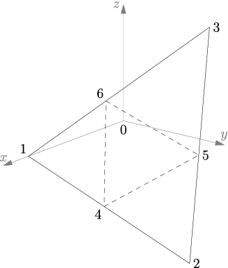
The procedure consists of splitting the face 123 into four new triangles by bisecting each edge, as shown in Figure 2, and integrating over the resulting sub-tetrahedra using the algorithm of the previous section. Given a tolerance , the convergence test is to check
| (27) |
where is the integral evaluated on the original tetrahedron, and , is the integral on each sub-tetrahedron. Sub-tetrahedra are 0146, 0425, 0536, and 0456. If the convergence criterion is not met, the sub-tetrahedra are split and the algorithm is applied recursively until the estimate of the total converges to the required tolerance. The effectiveness of this adaptive procedure will be demonstrated by numerical testing in Section 3.2.
2.4 Convergence
The error behaviour of the integration method can be investigated by considering an integral containing a polynomial source,
| (28) | ||||
which in the spherical coordinate system is
| (29) |
The error incurred by evaluating the integral numerically will depend on the geometry of the tetrahedron and on the details of the three quadrature rules used. To examine the error behaviour, we assume that can be integrated exactly. In this case, the error depends on the trigonometric integrals in and . We begin by developing an error estimate for the evaluation of
| (30) |
using an -point Gauss-Legendre quadrature. The quadrature rule integrates exactly the expansion of the integrand in Legendre polynomials up to order . Thus we derive an error estimate from the expansion of the integrand in Legendre polynomials,
| (31) | ||||
and is the Legendre polynomial. The first term neglected in the expansion of the integrand is and an upper bound on the error is . To estimate the coefficient , we write
| (32) | ||||
| (33) |
Use of tables [14, 7.324.2] gives
| (34) |
where is the Bessel function of the first kind. Using Equation 34, the coefficient is
| (35) |
To estimate the error bound, we use the large-order asymptotic form of the Bessel function [15, 10.19.1],
| (36) |
and hypothesize that for large the calculated integral should converge as
| (37) |
for some constant , which may depend on the geometry of the tetrahedron.
3 Results
Results are presented to demonstrate the performance of the quadrature algorithm in computing integrals over tetrahedra of various shapes. The first test integrals, which correspond to the evaluation of a volume potential such as the Biot–Savart law, are
| (38) |
computed for , with . The relative error is given as
| (39) |
where is the exact value found using an analytical method [8].
The geometries are chosen for comparison with previous work on a Duffy transformation method [12] and test the algorithms on tetrahedra whose geometries cause difficulties for numerical evaluation.
3.1 Basic algorithm
We first present results to assess the performance of the basic algorithm. The length of the Gauss-Legendre rules is varied, with in each calculation. For compatibility with previous work [12], three tetrahedra are considered. The first has nodes , , , and , with the height varied to examine the effect on the quadrature error. The second and third cases consider variations in the geometry of the base of the tetrahedron, Figure 3, to study possible effects of poorly-conditioned elements. In these cases, the node . In the second case, to study the influence of the vertex angle on the tetrahedron base. In the final test, the effect of the base aspect ratio is considered, by setting and varying .
Figure 4 shows integration error on different tetrahedra as a function of the number of quadrature points, including the convergence estimate, which is seen to fit the error very well.
As might be expected, in the case of a “well-conditioned” tetrahedron, in the upper plot, convergence is rapid and machine precision can be achieved. As is reduced, however, the method cannot achieve high accuracy with the number of quadrature points available and has quite poor results for . In the other two plots, the value of is held constant at 0.1 and the shape of the tetrahedron base is varied. Again, as the tetrahedron becomes more poorly conditioned, because of changes to the vertex angle or to the base aspect ratio, the quadrature scheme shows poor accuracy and unreliable convergence. The results of the next section will show how the adaptive version of the algorithm can overcome these defects and allow the method to converge to a required tolerance.
With regard to computational effort, Figure 5 shows the number of function evaluations for integration on tetrahedra of varying height, the same test case as in the first plot of Figure 4, using the spherical coordinate transformation and a Duffy transformation [12]. For a given quadrature rule length, the Duffy method has three times as many evaluation nodes as the spherical coordinate method, because of the decomposition of the tetrahedron in cylindrical coordinates [12, page 15], and this is accounted for in the operation count shown. For larger , i.e. better shaped tetrahedra, the spherical coordinate transformation gives more rapid convergence, with the Duffy method having better performance for , though the convergence rate is quite poor in both cases for small .
Comparison of all of the test case data with the corresponding data for a Duffy method [12, Figures 18–22] shows similar behaviour, though with slower convergence rates for the spherical coordinate method as the shape of the base triangle is changed. The convergence rate of the Duffy transform can be improved using further changes of variables [12]; in this paper we employ the adaptive approach of Section 2.3, tested in the next section. Overall, the computational effort for the Duffy-type methods is comparable to that of the method presented here, with the total number of integration points reaching values of the order of in order to achieve machine precision in some cases.
3.2 Adaptive algorithm
Results for the adaptive version of the algorithm are presented in Figure 6. In this case the tetrahedron nodes are , , , and with being changed to modify the conditioning of the tetrahedron. As before, an exact method is used to evaluate the integrals on the resulting tetrahedra. The adaptive algorithm is applied for three tolerances, and using Gaussian quadrature rules of length . Results presented are the total number of function evaluations required to reach the requested tolerance as a function of the tetrahedron conditioning represented by the height .
The results show the expected convergence behaviour. For , any of the quadrature rules gives a solution to the required tolerance, as for the basic algorithm evaluated in the previous section, but as is reduced and the tetrahedron becomes more poorly conditioned, the method needs a greater number of recursions to achieve convergence. At small values of and , this leads to a large number of function evaluations. In all cases, however, the requested tolerance is achieved, even when quite low-order Gaussian quadratures, , are used to integrate on sub-elements. Numerical tests for accuracy when the base shape is modified give similar results with convergence roughly independent of aspect ratio and vertex angle and are not presented here.
It is interesting to note that the low-order rules can require more function evaluations to achieve a given tolerance than higher order rules, in particular, for . This appears to happen because for the well-conditioned tetrahedron, the low-order rules can require more recursion levels to reach the convergence criterion.
We hypothesize that the adaptive algorithm achieves good convergence because the base splitting shown in Figure 2 has the effect of generating four tetrahedra which are better conditioned than the parent element by virtue of having smaller area bases with a constant height, in effect increasing with a corresponding improvement in the element conditioning.
3.3 Non-integer
The previous sections show how the proposed algorithm works for an integrand with integer , where a reference value can be evaluated exactly using analytical methods. This is an important case in many applications, but there are also problems where non-integer values appear. Here, we consider two cases, which arises in crack problems in solid mechanics, and an irrational value of which poses particular difficulties for coordinate transformation schemes.
In the first case, that of rational , a Duffy-type transformation [12] can eliminate the singularity and allow Gauss-Legendre rules to be used in the radial direction. Figure 7 shows the performance of the method compared to the evaluation of a reference integral using the Duffy-type method [12] with high order Gaussian quadratures. The integral is evaluated on a tetrahedron with nodes , , , and . The Duffy transformation was applied to the integral using high-order Gauss-Legendre rules to give a reference value, and the method of this paper was implemented using Gauss-Legendre rules in and and a Gauss-Jacobi rule for . In the non-adaptive case, the computational effort for the spherical coordinate method is about the same as for the Duffy transformation, though adaptive quadrature incurs a computational cost to ensure convergence to the required tolerance, as shown by the shift of the data points to the right.
Finally, we consider a case similar to that used in previous work [16], with an irrational value of which is close to the point where the integrand is not integrable. We set and integrate using a quadrature with . This integral cannot be evaluated using the Duffy-type coordinate transformation, since it requires a rational value of , so convergence is tested by evaluating
| (40) |
where is the integral evaluated using quadrature rules of length 20, or function evaluations, in the spherical coordinate method. Figure 8 shows against the total number of function evaluations for the same tetrahedron geometry as in Figure 7. In order to track the convergence of the integral, a single monomial source term is used, evaluating as defined in Equation 38.
3.4 Evaluation of Biot–Savart integral
The final numerical test evaluates the performance of the integration method in a realistic application, the evaluation of the Biot–Savart integral in three dimensions. This is an application which has motivated the development of a number of integration techniques [2, 7, 9, for example] because of its importance in fluid dynamics and electromagnetism. Here we evaluate the velocity field of a vortex ring, a basic component of many flows [17]. The velocity induced by a three-dimensional distribution of vorticity over a volume is given by [18, page 18]
| (41) | ||||
For an axisymmetric ring, we employ cylindrical coordinates ,
| (42) | ||||
| (43) |
In the axisymmetric case, vorticity has only an azimuthal component and the radial and axial velocity components are given by [18, page 21],
| (44a) | ||||
| (44b) | ||||
| (44c) | ||||
where and are complete elliptic integrals of the first and second kind respectively. Equations 44 can be used to evaluate a reference velocity for comparison with the evaluation of Equation 41. As a test case, we use a Gaussian-core ring with
| (45) | ||||
| (46) |
and .
For the three-dimensional evaluation, the vorticity is discretized on an unstructured tetrahedral mesh with , , , using the tetgen code [19], and the velocity field is evaluated at each node of the tetrahedralization. Integration over tetrahedra is performed using the high-order quadrature rules of Jaskowiec and Sukumar [20], except for tetrahedra which have an evaluation point as a vertex. In this case, the integral over the tetrahedron is evaluated using the method of Section 2. For comparison with the axisymmetric formulation, the velocity is evaluated at , , where . Figure 9 shows the radial and axial velocity evaluated using the axisymmetric formulation. The lower plot shows a zoom of the axial velocity evaluated using only fixed node quadratures [20] and the singular quadrature method of this paper. The difference between the two plots is clear and demonstrates the requirement for properly handling of the singular integrand.
Error in the calculation is controlled by the discretization of the domain, by the order of the fixed node quadrature rules, and by the order of the singular quadrature rules. The error measure used is
| (47) |
where is the axial velocity computed using Equations 44, and that computed using the three-dimensional integration over tetrahedra.
;
Summation over the fixed quadrature points was performed using a fast multipole method (FMM) based on the approach of Gumerov and Duraiswami [21, 22, 23]. Direct summation was used at a set of sample points to check that the truncation error of the FMM summation was at least an order of magnitude less than the difference between the computed and reference velocities.
The error in the evaluated velocity is given in Figure 10, which shows the error measure of Equation 47 against the number of singular integration points, as a function of the mesh discretization. For these results, the twelfth order symmetric quadrature rule [20] was used for the non-singular tetrahedron integration. As expected, meshes with a greater number of nodes achieve a smaller error, though they require more quadrature points to do so. The discretization error limit is reached for a smaller number of quadrature nodes for coarser meshes than for the more refined.
| 11 | 23 | 44 | 74 | 117 | |
|---|---|---|---|---|---|
| None | |||||
| 8 | |||||
| 27 | |||||
| 64 | |||||
| 125 | |||||
| 216 | |||||
| 343 | |||||
| 512 | |||||
| 729 | |||||
Table 1 gives the error in evaluation of the velocity on the finest mesh tested, as a function of the number of singular and fixed quadrature points. In this case, the accuracy is limited by the number of quadrature points The first row of the table shows the error when the singular quadrature is not used and only the non-singular method is applied. Lower rows show the effect of including increasingly high-order singular rules and show that the minimum error for a given non-singular quadrature is achieved when the number of singular nodes is 2–3 times the number of non-singular nodes .
4 Conclusions
A method has been presented for the evaluation of integrals on a tetrahedron with an integrable singularity at one vertex, motivated by the evaluation of volume integrals used in fluid dynamics and electromagnetism, and in fracture mechanics. The algorithm has been shown to be reliable for well-conditioned tetrahedra in its basic form. Extended to an adaptive form, it can compute the volume integral to a required tolerance, even when the tetrahedron is poorly conditioned. The method uses standard tools, such as one-dimensional Gauss quadratures and simple geometric transformations, and can be used without difficulty in production codes.
References
- [2] Urankar, L.K.: Vector potential and magnetic field of current-carrying finite arc segment in analytical form, part IV: General three-dimensional current density. IEEE Transactions on Magnetics 20(6), 2145–2150 (1984)
- [3] Weggel, C.F., Schwartz, D.P.: New analytical formulas for calculating magnetic field. IEEE Transactions on Magnetics 24(2), 1544–1547 (1988)
- [4] Onuki, T., Wakao, S.: Systematic evaluation for magnetic field and potential due to massive current coil. IEEE Transactions on Magnetics 31(3), 1476–1479 (1995)
- [5] Graglia, R.D.: Static and dynamic potentials for linearly varying source distributions in two- and three-dimensional problems. IEEE Transactions on Antennas and Propagation AP-35(6), 662–669 (1987)
- [6] Wilton, D.R., Rao, S.M., Glisson, A.W., Schaubert, D.H., Al-Bundak, O.M., Butler, C.M.: Potential integrals for uniform and linear source distributions on polygonal and polyhedral domains. IEEE Transactions on Antennas and Propagation AP-32(3), 276–281 (1984)
- [7] Suh, J.-C.: The evaluation of the Biot–Savart integral. Journal of Engineering Mathematics 37, 375–395 (2000). https://doi.org/10.1023/A:1004666000020
- [8] Carley, M., Angioni, S.: Exact integration of surface and volume potentials. Journal of Engineering Mathematics 104, 93–106 (2017). https://doi.org/10.1007/s10665-016-9875-5
- [9] Marshall, J.S., Grant, J.R., Gossler, A.A., Huyer, S.A.: Vorticity transport on a Lagrangian tetrahedral mesh. Journal of Computational Physics 161(1), 85–113 (2000). https://doi.org/10.1006/jcph.2000.6490
- [10] Duffy, M.G.: Quadrature over a pyramid or cube of integrands with a singularity at a vertex. SIAM Journal of Numerical Analysis 19(6), 1260–1262 (1982)
- [11] Khayat, M.A., Wilton, D.R.: Numerical evaluation of singular and near-singular potential integrals. IEEE Transactions on Antennas and Propagation 53(10), 3180–3190 (2005). https://doi.org/10.1109/TAP.2005.856342
- [12] Lv, J.-H., Jiao, Y.-Y., Feng, X.-T., Wriggers, P., Zhuang, X.-Y., Rabczuk, T.: A series of Duffy-distance transformation for integrating 2D and 3D vertex singularities. International Journal for Numerical Methods in Engineering 118, 38–60 (2019). https://doi.org/10.1002/nme.6016
- [13] Cano, A., Moreno, C.: Transformation methods for the numerical integration of three-dimensional singular functions. Journal of Scientific Computing (2017). https://doi.org/10.1007/s10915-016-0311-9
- [14] Gradshteyn, I., Ryzhik, I.M.: Table of Integrals, Series, and Products, 5th edn. Academic, London (1980)
- [15] National Institute of Standards and Technology: Digital Library of Mathematical Functions. http://dlmf.nist.gov/ (2010)
- [16] Chernov, A., von Petersdorff, T., Schwab, C.: Quadrature algorithms for high dimensional singular integrands on simplices. SIAM Journal of Numerical Analysis 70, 847–874 (2015). https://doi.org/10.1007/s11075-015-9977-6
- [17] Shariff, K., Leonard, A.: Vortex rings. Annual Review of Fluid Mechanics 24, 235–279 (1992)
- [18] Danaila, I., Kaplanski, F., Sazhin, S.S.: Vortex Ring Models. Springer, Cham, Switzerland (2021)
- [19] Si, H.: TetGen, a Delaunay-based quality tetrahedral mesh generator. ACM Transactions on Mathematical Software 41(2) (2015). https://doi.org/10.1145/2629697
- [20] Jaśkowiec, J., Sukumar, N.: High-order symmetric cubature rules for tetrahedra and pyramids. International Journal for Numerical Methods in Engineering 122, 148–171 (2021). https://doi.org/10.1002/nme.6528
- [21] Gumerov, N.A., Duraiswami, R.: Recursions for the computation of multipole translation and rotation coefficients for the 3-D Helmholtz equation. SIAM Journal on Scientific Computing 25(4), 1344–1381 (2003). https://doi.org/10.1137/S1064827501399705
- [22] Gumerov, N.A., Duraiswami, R.: Fast Multipole Methods for the Helmholtz Equation in Three Dimensions. Elsevier, Oxford (2004)
- [23] Gumerov, N.A., Duraiswami, R.: Comparison of the efficiency of translation operators used in the fast multipole method for the 3D Laplace equation. Technical Report CSTR 4701, UMIACS TR-2005-09, University of Maryland (2005)