Prestressed elasticity of amorphous solids
Abstract
Prestress in amorphous solids bears the memory of their formation, and plays a profound role in their mechanical properties, from stiffening or softening elastic moduli to shifting frequencies of vibrational modes, as well as directing yielding and solidification in the nonlinear regime. Here we develop a set of mathematical tools to investigate elasticity of prestressed discrete networks, which disentangles the effects from disorder in configuration and disorder in prestress. Applying these methods to prestressed triangular lattices and a computational model of amorphous solids, we demonstrate the importance of prestress on elasticity, and reveal a number of intriguing effects caused by prestress, including strong spatial heterogeneity in stress-response unique to prestressed solids, power-law distribution of minimal dipole stiffness, and a new criterion to classify floppy modes.
I Introduction
Almost all solid materials are stressed. Amorphous solids exhibit quenched residual stress from their preparation process, crystalline solids are stressed by defects and grain-boundaries, and living matter experiences active stress from biological processes. The ubiquity of stressed solids is encapsulated in the fact that the stress tensor , as a symmetrical matrix in dimensions, has independent degrees of freedom, but the force balance equation,
| (1) |
only poses constraints, leaving unconstrained components in the stress field. In absence of external load, all components have to vanish if the material, and the stress field, have to be homogeneous, but they can be nonzero at lengthscales over which heterogeneities or excess constraints are present (“geometric frustration”), giving rise to prestress, (also known as “residual stress”, “initial stress” or “eigenstress” in different contexts) Alexander 1998; Ulm and Coussy 2003.
In structural engineering, prestress is proactively used to modify both stability and load bearing capability of structures, from prestressed reinforced concrete to tensegrity architectures [Fig. 1 (a), (h) and (j)]. In materials, instead, prestresses can emerge spontaneously, as the direct consequence of out-of-equilibrium processes through which they solidify, or of the external load applied during processing. Prominent examples include isotropic compressive prestress in jammed packings Wyart et al. 2005 or gels Bouzid et al. 2017, shear prestress in shear jammed granular matter Bi et al. 2011 and shear thickened dense suspensions Sehgal et al. 2019, isotropic prestresses in glasses Ballauff et al. 2013, and rich varieties of anisotropic prestress fields in prestressed/tensegrity metamaterials Gei et al. 2009; Chen et al. 2012; Fraternali et al. 2014; Meeussen et al. 2020; Merrigan et al. 2021 and biological systems Armon et al. 2011; Wyczalkowski et al. 2012; Feng et al. 2018 [Fig.1 (b)-(g) and (i)]. Remarkably, very much in the same way as for buildings and large scale structures, microscopic residual stresses in amorphous solids may strongly affect their strength—stiffen or soften them, and direct how they fail Alexander 1998; Zhang et al. 2017; Ozawa et al. 2018; Vasisht et al. 2020; Barlow et al. 2020; Berthier et al. 2019. In addition, prestress stores elastic energy in materials, which then feature a different energy landscape when compared to stress-free materials Debenedetti and Stillinger 2001; Manning and Liu 2011; Ninarello et al. 2017; Vasisht et al. 2021; Bhaumik et al. 2021; Richard et al. 2020.

A deep understanding of the consequences of prestress is therefore key to predict elasticity and material properties in general, but microscopic prestresses can be very elusive, since it is difficult to directly access them in experiments and in most cases only their indirect consequences can be detected. It has been shown that, in jamming of frictionless particles, compressive prestress both stabilizes the packing by maintaining particle contacts, and destabilizes it by shifting frequencies of vibrational modes Wyart et al. 2005; DeGiuli et al. 2014, as well as control the response to external forces Ellenbroek et al. 2009. In biological systems such as biopolymer gels and epithelial cell sheets, tensile stress has been shown to provide stability Licup et al. 2015; Feng et al. 2015; Feng et al. 2016; Noll et al. 2017; Hardin et al. 2018; Yan and Bi 2019; Merkel et al. 2019; Liu et al. 2021a, and active stress generated by molecular motors has been shown to give rise to sophisticated effects on rigidity Alvarado et al. 2013 and mechanical signal transmission Ronceray et al. 2016.
However, a general theoretical framework to disentangle effects of microstructure and prestress, and map how external load is carried by prestressed amorphous solids, is still missing. Many studies of elasticity of amorphous solids have mainly focused on determining how the disorder in their microstructure affects elasticity Tanguy et al. 2002a; O’Hern et al. 2003; Zaccone and Scossa-Romano 2011; Liu and Nagel 2010, whereas the role of prestress is far less understood, so that there is a gap in the theoretical approaches that can rationalize the mechanics of amorphous solids when it comes to prestress. In a granular solid, the same configuration of particles and the same value of the stress at the boundary are compatible with multiple stress distributions, which correspond to the so-called “force network ensemble” Snoeijer et al. 2004; Tighe et al. 2008; Tighe et al. 2010; Bi et al. 2015 and is related to the broader concept of the “Edwards ensemble” Edwards and Oakeshott 1989 where both microscopic configuration and stress are allowed to vary for a given boundary stress. Statistical relations of prestress distributions in this type of ensembles have been recently discussed, and force-balance constraints [Eq. (1)] have been shown to produce intriguing long-range correlations Mao et al. 2007; Henkes and Chakraborty 2009; Mao et al. 2009; Lemaître 2017; Maier et al. 2017; DeGiuli 2018; Nampoothiri et al. 2020. Nevertheless, unraveling the role of disordered configurations and disordered prestress in the mechanical properties of amorphous solids has remained difficult both conceptually and computationally.
When considering the stress distributions in a mechanically stable structure, the concept of states of self stress (SSSs) Calladine 1978; Pellegrino and Calladine 1986 captures their eigenstates that leave all components of the solid structure in force balance. In discrete mechanical networks, SSSs originate from redundant constraints. SSSs were first introduced in mechanical engineering to describe load bearing abilities of structures, and more recently used by the condensed matter physics community for their role in characterizing mechanical topological edge states Sun et al. 2012; Kane and Lubensky 2014; Lubensky et al. 2015; Mao and Lubensky 2018. Because SSSs span the linear space of all possible ways a system can carry load, mapping out, and further programming, this SSSs linear space offers a convenient handle to control the mechanical response of materials. Interesting examples of this type include recent work on programming SSSs using topological mechanics to direct buckling and fracturing of metamaterials Paulose et al. 2015; Zhang and Mao 2018. Intriguingly, SSSs in jammed packings have been shown to exhibit rich spatial structures and a divergent length scale near jamming Sussman et al. 2016. Some of these findings suggest that SSSs may be the natural tool to rigorously quantify the effect of prestress distributions on material properties, but a direct connection remains to be built.
Here we present a systematic method to investigate how prestress affects the mechanical response of amorphous solids, based on the concept of SSSs, where the configuration and the prestress are allowed to change independently, while force-balance is always maintained. As we discuss below, prestress is a linear combination of the SSSs of the stress-free version of the mechanical network, and leads to a new set of SSSs, capturing the unique, prestress-controlled, mechanical response of the system. By applying this method to a prestressed triangular lattice model and a computational model of amorphous solids, we show that prestress greatly enlarges the linear space of stress-bearing states, and that a number of intriguing effects arise where prestress strongly controls the mechanical response, both at the local and the global level.
The general method we introduce here is applicable to a wide range of systems, ordered and disordered, where prestress affects elasticity. It provides an efficient computational algorithm for finding the stress distribution when the system is under any load, as well as offering a platform to develop a field-theoretic treatment of prestressed elasticity of amorphous solids. Because this method allows the microstructure and the prestress field to vary separately, it offers a pathway to investigate how amorphous solids evolve as well as develop memory under stress without changing their configuration. We demonstrate the method using a triangular lattice model with varying prestress, and test it in amorphous configurations of compressed repulsive particles, obtained through numerical simulations. In such model solids, we show how prestress determines their response to both macroscopic shear strain and local dipole forces, and show that they display qualitatively different behaviors from unstressed spring networks with the same geometry. Finally, for the model solids obtained through computer simulations, we use the new method to study the dependence of the stress-bearing ability on the preparation protocol, which changes the microscopic prestress distribution, as well as various signatures of the spatial evolution of the stress under a shear strain.
Overall, the new method proposed here is an ideal candidate to investigate the nature of rigidity transitions in prestressed systems, and furthermore, yielding and shear thickening/thinning systems such as granular matter or jammed packings and dense suspensions, to potentially shed new light on the dynamical interplay between stress and geometry in these complex materials.
The paper is organized as follows. In Sec. II we review the fundamental theories of prestressed mechanical networks. In Sec. III we introduce a new formulation of equilibrium and compatibility matrices in prestressed networks, and discuss how they control both zero modes and stress response. In Sec. IV we use a prestressed triangular lattice model to illustrate how prestress controls the vibrational modes and the stress response. In Sec. V we apply these methods to analyze the stress response of a computational model of prestressed amorphous solids, and Sec. VI contains a summary and outlook.
II Prestressed mechanics
In this section we briefly review mechanics of prestressed networks, their continuum elasticity limit, as well as how prestress affects rigidity of discrete networks in general.
II.1 Prestressed mechanical networks
We consider a discrete network of point-like particles connected by pairwise central-force potentials (bonds). When this network is deformed, particle , which was originally at in the reference state, undergoes a displacement to a new position
| (2) |
The change of the elastic energy associated with this deformation, of a bond connecting particles , is , where , are the vectors along the bond in the reference state and the deformed state respectively.
This change in energy can be expanded to quadratic order in [using Eq. (2)]
| (3) |
where the derivatives are taken at , and is the difference of displacement vectors of the two particles connected by bond , and
| (4) |
are its components parallel and perpendicular to the original bond direction , respectively.
The derivatives of this potential,
| (5) |
correspond to the spring constant and the pretension (tension of the bond in the reference state, where stands for “prestress”) of bond .
In a stress-free network, all bonds are at their rest length and thus , leaving only the term in Eq. (3). Vibrational modes of disordered networks of this type have been extensively studied, yielding a rich set of interesting phenomena including quasilocalized modes, anomalies of density of states at low frequencies, etc. Tanguy et al. 2002a; O’Hern et al. 2003; Wyart et al. 2005; Wyart et al. 2008; Liu and Nagel 2010; Chen et al. 2011; Lerner et al. 2012; Mosayebi et al. 2014; Stanifer et al. 2018.
When a network is prestressed, , and both terms contribute to the elastic energy, increasing the number of microscopic constraints, as we discuss in detail in Sec. III. Interestingly, in general the sign of can be either positive (tension) or negative (compression). In the case of , the prestress term contribute with another complete square term to the elastic energy, clearly stabilizing the system. In the case of , naively, the prestress term appears to be unstable. However, because are not variables independent of (of other bonds), the stability of the network needs to be analyzed in terms of the collective modes, which we discuss more in Sec. II.3.
Here we assumed that the network in the reference state is in force balance, i.e., the total force on each particle vanishes. As a result, there is no term in the expansion of the elastic energy. Note that the force-balance condition and the stress-free condition are two distinct conditions, where the later means on all bonds, and is a much more stringent requirement than the force-balance condition. We will revisit this distinction in continuum elasticity in Sec. II.2.
II.2 Continuum elasticity with prestress
The discrete theory discussed above can be rigorously linked to continuum elasticity using the relation between the discrete nonlinear strain of bond defined as Born et al. 1955; DiDonna and Lubensky 2005
| (6) |
and the (continuum) nonlinear right Cauchy-Green strain tensor (repeated indices are summed over)
| (7) |
where the relation reads
| (8) |
This follows from the definition of the nonlinear strain tensor, and we have taken the continuum limit by assuming that the spatial variation of the strain field is small over the scale of the particles and bonds, so that the deformation of bond is determined by the strain at its location .
By expanding the bond length in terms of , we can rewrite the expansion of the elastic energy of bond as
| (9) |
This is equivalent to the expansion in Eq. (3), by recognizing that
| (10) |
The combination of Eqs. (8) and (9) allows us to write the bond energy change in terms of the strain tensor.
The elastic energy of the whole system can be taken to the continuum limit by converting the sum over all bonds to an integral over space
| (11) |
where the space is Voronoi tessellated according to the particles, and is the volume of the Voronoi cell at , and the overall factor of comes from the fact that every bond is counted twice. The sum in the continuum limit represent the sum over the bonded neighbors of the particle at . Using this formulation, the elastic energy of the system can be written in the conventional form
| (12) |
where the local elastic-modulus tensor and prestress field are determined from the discrete network by
| (13) |
where the sum is over all connected neighbors of particle , which is at position , and . From this relation, it is clear that the prestress field in the continuum theory comes from pretensions on bonds which are not at their rest length in the discrete network, whereas the elastic-modulus tensor depends on both the spring constants and the tensions.
The body-force in this continuum theory
| (14) |
corresponds to the total force on each particle (normalized by the volume of the Voronoi cell) in the discrete network. Thus, the force-balance conditions in the discrete network and the continuum theory are indeed the same condition.
It is often useful to write this continuum theory in a quadratic expansion in terms of the displacement field ,
| (15) |
where we have used the symmetry of and the force balance condition which eliminates terms in this elastic energy.
II.3 Prestressed rigidity
The concept of “rigidity” has been a central theme in the discussion of mechanics of soft materials. In general, rigidity can be interpreted from two viewpoints, (i) a microscopic one, where rigidity is attributed to the vanishing of floppy modes (i.e. modes of deformation that cost no elastic energy) Maxwell 1864; Tay and Whiteley 1984, and (ii) a macroscopic one, where rigidity is defined as the emergence of a spanning rigid cluster that can transmit stress Jacobs and Thorpe 1995. Remarkably, these two rigidity criteria coincide for the jamming transition of frictionless repulsive particles Liu and Nagel 2010.
In this section we focus on the first viewpoint and discuss how prestress changes floppy modes. In Sec. III we discuss how prestress affects the ability of the system to carry additional loads (second point of view) with the help of the concept of SSSs.
Rigidity of stress-free discrete mechanical networks is often analyzed via the comparison between the numbers of constraints and degrees of freedom Maxwell 1864; Jacobs and Thorpe 1995. This is well summarized by the Maxwell-Callandine index theorem Calladine 1978; Sun et al. 2012. Rigorously speaking, when this theorem determines that the number of floppy modes of a system vanishes, it implies that the system is “first-order rigid”, where the energy increases quadratically for all deformations. By contrast, in a “second-order rigid” system the leading order expansion of the energy with respect to some deformations is of higher order such as cubic or quartic Connelly and Whiteley 1992; Connelly and Whiteley 1996.

How does prestress change this paradigm of rigidity? It was pointed out in Ref. Connelly and Whiteley 1992; Connelly and Whiteley 1996 that prestress can rigidify second-order rigid systems and make all their modes first-order rigid. Interestingly, this prestress stabilization effect can even take place in systems which are underconstrained according to the (stress-free) Maxwell counting. One simple example is the honeycomb lattice, which has coordination number and is thus significantly below the Maxwell point of ( being the spatial dimension) where degrees of freedom and constraints balance. When a honeycomb lattice is under tension, all modes are lifted to finite frequency (except for trivial translations). It is worth noting that this example does not violate the theorems in Ref. Connelly and Whiteley 1996: although underconstrained, floppy modes of the honeycomb lattice under periodic boundary conditions are in fact second order rigid. In Fig. 2 we show examples of how networks become rigid by prestress.
This effect has been studied in various disordered mechanical networks from polymer gels to jamming of particles and biological tissues Wyart et al. 2008; Licup et al. 2015; Feng et al. 2016; Vermeulen et al. 2017; Merkel et al. 2019; Damavandi et al. 2021. In these models, the underconstrained network typically exhibit an extensive number of floppy modes before the application of stress. When certain types of strain (tensile or shear) is applied to the network, a system spanning SSS emerges and becomes stressed, providing (macroscopic) rigidity and thus elastic moduli. This prestress also rigidifies floppy modes in the network, as the geometry of the network evolves and these modes become second order rigid.
Interestingly, by increasing the magnitude of the prestress, a stable network can also destabilize. This happens when the negative terms in Eq. (3), due to compressed bonds, compete with the positive terms and creates negative eigenvalues in the dynamical matrix. Some examples of this effect are also shown in Fig. 2. As we introduce our new mathematical tools in Sec. III, we discuss this effect in more detail.
III States of self-stress in stressed elasticity
Now we introduce a new (equilibrium and compatibility) decomposition for the mechanics of prestressed systems, that can be used to analyze their SSSs and zero modes (ZMs). We first briefly review this decomposition for stress-free systems, and then discuss the more general case of prestressed systems. We also develop a general formulation of these SSSs to compute mechanical response to an external load, including both macroscopic strain and local forces.
III.1 States of self-stress in stress-free systems
The elastic energy of a stress-free network of point-like particles connected by central-force springs in dimensions can be written to quadratic order in using the dynamical matrix as
| (16) |
where the inner product is taken in the dimensional space for particle displacements , and the superscript “” on the dynamical matrix signifies that this dynamical matrix describes a stress-free system where only enters the elastic energy. The more general form for prestressed systems will be discussed in Sec. III.2. This quadratic form can be decomposed into two steps using the equilibrium and compatibility matrices, defined as
| (17) | ||||
| (18) |
Here and represent the extension and tension of every bond, which are both dimensional vectors, and the superscript “” indicated that they are along the bond direction. and represent the displacement and total force on every site, which are both dimensional vectors. As a result, the equilibrium matrix has the dimension , and the compatibility matrix has the dimension . The two matrices are in fact transpose of one another, . Note we take the convention that denotes tension and denotes compression. This is consistent with the minus sign of Eq. (18), as is the force exerted by the bonds in the networkon the sites.
Using these relations in Eq. (16), it is straightforward to see that
| (19) |
where is a diagonal matrix that contains all the spring constants . In the sign convention we use here, Hookian’s law on the springs takes the form , as extension causes tension on the springs.
The null space of is the set of tensions, called SSSs, that produce no forces at any site,
| (20) |
The null space of is the set of site displacements, called ZMs, that produce no changes in bond lengths,
| (21) |
Floppy modes are a subset of ZMs excluding trivial rigid body motions of the whole system, and have been extensively studied in soft matter systems, due to their obvious significance as capturing deformations with no cost of elastic energy. SSSs have only recently been explored in soft matter, but also show great potential in characterizing stress-bearing structures in mechanical networks Lubensky et al. 2015; Sussman et al. 2016.
Applying rank-nullity theorem on matrices leads to the Maxwell-Calladine index theorem Calladine 1978; Sun et al. 2012
| (22) |
where are the numbers of ZMs and SSSs.
These concepts have found wide applications recently in the new field of topological mechanics, as and can become topologically protected modes in Maxwell lattices and networks Kane and Lubensky 2014; Lubensky et al. 2015; Rocklin et al. 2017; Zhang and Mao 2018; Zhou et al. 2018; Ma et al. 2018; Mao and Lubensky 2018; Zhou et al. 2019; Zhou et al. 2020; Sun and Mao 2020.
III.2 States of self-stress in prestressed systems
Prestress on a force-balanced mechanical network can always be viewed as “exciting” an existing SSS in the “stress-free version” of the same network (which is generated by turning off stress in the prestressed network but keeping exactly the same geometry—requiring to redefine the rest-length of the springs). Thus, the stress-free version of a prestressed network must exhibit a SSS in the first place.
With prestress, the elastic energy includes both and terms as analyzed in Eq. (3),
| (23) |
Similar to the stress-free case, using the fact that this elastic energy consists only of complete square terms, this dynamical matrix can also be decomposed into matrices,
| (24) |
where
| (25) |
defines the new matrix and . Here we have defined the new dimensional vector which contains one component from and from for each of the bonds. It is worth noting here that the compatibility matrix is now dimensional instead of dimensional, because this matrix maps the dimensional displacement vector of the network into and for each bond . At the same time, the equilibrium matrix is dimensional. The spring constant matrix is a diagonal matrix with spring constant for the terms and pre-stress for the terms,
| (26) |
where there are blocks of dimensional diagonal matrices (one longitudinal and transverse).
These new matrices describe the mapping between the ( dimensional) degrees of freedom space and the (now dimensional) constraint space. In parallel with Eq. (25) we have
| (27) |
Correspondingly, and are the parallel and perpendicular components of .

It might appear confusing how tension on a central-force spring can have a component perpendicular to the spring. This can be understood by realizing that the and components are defined with respect to the reference configuration, and denotes an increment of stress in addition to the prestress . In the prestressed reference state, is along bond in the reference configuration . In the state after the (infinitesimal) deformation, the total tension is along bond in the deformed configuration . These two bond directions, and , are not parallel in general. The field in Eq. (27) represents the increment from the pretension to the tension after the deformation, and thus has components parallel and perpendicular to the original bond direction. In other words, under an (infinitesimal) deformation, both bond (parallel) extension and bond rotation cause increment of stress [Eq. (III.2)], and the two components are and respectively.
SSSs in a prestressed system are thus defined as any vectors that satisfy
| (28) |
which represent respectively parallel and perpendicular change of bond tensions that leave all particles in force balance, for a prestressed network. In Fig. 3 we show two examples of mechanical networks where prestress introduces extra SSSs that involve components. This formulation characterizes the tensegrity phenomena Calladine 1978; Connelly and Whiteley 1992 where prestress generates new SSSs for the system to carry other types of load.
III.3 Zero modes in prestressed systems
Prestressed systems have two types of ZMs, type , which leave on all bonds, and type , which violate this relation but are still zero energy modes. In this section we discuss both types of ZMs.
Type ZMs in prestressed networks can be defined as modes that live in the null space of ,
| (29) |
The number of this type of ZMs satisfy the Maxwell-Calladine index theorem for a stressed network, which can be proven by applying the rank-nullity theorem on the new matrices,
| (30) |
Note that the last term is now for the prestressed network instead of in the stress-free case. More rigorously, if we also consider the possibility that not all bonds are stressed, this index theorem should be written as
| (31) |
where each unstressed bonds only provide one constraint.
Type ZMs in prestressed systems are not included in Eq. (29). Instead, they are ZMs due to the fact that some spring constants in are negative (from compressively prestressed bonds), and their contribution can cancel out the positive terms. They are “fine-tuning” ZMs which are only zero energy when the prestress satisfies certain conditions so that the positive and negative terms exactly cancel. This is also the point when varying the magnitude of the prestress starts to cause instability, as we discuss at the end of Sec. II.3. One example of such mode is shown in Fig. 2. Interestingly, because and , type ZMs lead to a set of SSSs . One trivial example of this type of ZMs is the rigid rotation of the network if the system is under open boundary conditions: the rotation causes and thus does not satisfy Eq. (29), but it is indeed a ZM of the dynamical matrix (this ZM does not require fine tuning of stress but all other type B ZMs do). A nontrivial example of such fine-tuning ZMs is shown in Fig. 2e where the sum of and terms in the elastic energy vanish. Type ZMs are not included in the Maxwell-Calladine index theorem for prestressed systems [Eq. (30)].
Remarkably, although ZMs in prestressed systems are more complicated as we discussed above, the definition of SSSs in Eq. (28) is robust as it relies only on force balance, and is not affected by the positive definiteness of . In our discussions below, we mainly focus on these SSSs and show how they form a linear space that efficiently characterizes how load is carried by a prestressed system.
III.4 Stress response to homogeneous load
One important property of SSSs is that they form a linear space containing all possible ways a network can carry stress while keeping all particles in force balance. Thus, when the network is under load, actual stress distributions must come from linear combinations of SSSs, and the linear space of SSSs characterizes the capability of a system to carry any external load. It is worth pointing out here that we refer to external loads that do not “introduce new constraints” to the system, and the meaning of this condition will become clear in the end of Sec. III.5.
Here we first illustrate this formulation using a simple shear on a stress-free network with all spring constants being 1. The bond tension in response to this shear can be decomposed in the SSSs linear space because this space form a complete basis for all force-balanced stress distributions, as we discussed above. The decomposition can be written as
| (32) |
where is the bond extension if the strain were affine (i.e., homogeneous shear strain). The sum runs in the dimensional linear space of all SSSs, . This relation is straightforward to prove as follows: when a strain is imposed on the system (e.g., via Lees-Edwards boundary conditions in a computational model, or in the bulk of a mechanical network strained from the boundary), in addition to affine bond extensions , the system responds by particle displacements (e.g., nonaffine deformations) to minimize the elastic energy while maintaining this macroscopic strain, so the resulting bond extensions are
| (33) |
If all spring constants are 1, we have . As we mentioned above, must belong to the SSSs linear space, and the linear combination coefficients are
| (34) |
The second term has to vanish because . This proves the decomposition in Eq. (32).
Three comments can be made from this result. First, if the shear strain has no overlap with any SSSs in the system, for all , the system can not carry the load. What would happen physically is that the system yields until a new SSS, able to carry that load, emerges. Second, the same approach can also be applied to other types of load, such as a hydrostatic pressure. It is important to note here that any component in the imposed strain that can be written in terms of will not cause stress—it corresponds to strain that will be relaxed by degrees of freedom available to the system. Third, a similar formulation can also be developed with loads applied via specifically controlled boundary displacements, where SSSs are defined as bond tensions leaving internal sites in force balance, and the strain can be applied from bonds connected to boundaries Zhang and Mao 2018.
The relation is slightly more complicated when the spring constants are different for each spring,
| (35) |
where is the inverse of the spring constant matrix projected to the SSS linear space (see detailed definition in App. A).
This relation can readily be generalized to the pre-stressed case, where
| (36) |
A detailed proof of this relation is included in App. A. It is worth noting that the response calculated here is the addition to the prestress in response to the load, so the total stress in the system is where only has longitudinal components and has both longitudinal and transverse components (with respect to the bond direction in the prestressed reference state).
III.5 Stress response to force dipoles
Similar projections can also be applied to compute the stress response of a prestressed system to local forces, such as a force dipole acting on a bond.

The main difference between this case of a force dipole and the external strain case discussed in Sec. III.4 is that the force-balance condition here needs to include the external forces,
| (37) |
where is the externally imposed force and is the tension response of the system, which causes . cancels with , leaving the system in force balance.
When the external forces take the form of a force dipole on a bond , they can be written as
| (38) |
where is a vector in the bond space with 1 on the bond where the dipole is imposed, and 0 on all other bonds. This sets the magnitude of the dipole force to be , the value of which is irrelevant for the linear theory. The sign convention of this equation follows from Eq. (27) where causes . Combining Eqs. (37) and (38) we have
| (39) |
indicating that the total tension field (sum of the external dipole and the network response) is a SSSs of the network. The response can then be derived using a similar method as discussed in Sec. III.4, and we have (as detailed in App. B)
| (40) |
In the simple case of (all springs having the same spring constant which only applies to stress-free networks), the second term on the right hand side of the equation reduces to the “quasi-localized SSSs” defined in the stress-free case, characterizing dipole responses Sussman et al. 2016; Lerner 2018. Here we extend this concept to prestressed networks, and our formulation can be used to not only compute dipoles with force along the bond, but also “transverse” or “tilted” dipoles where the force pair is perpendicular or in an arbitrary angle to the bond (see example in Fig. 4).
A “dipole stiffness” can then be defined to characterize this response
| (41) |
where serves the purpose of projecting the force and displacements to the direction of the external force dipole. A different version of (longitudinal only) dipole stiffness has been introduced in Ref. Rainone et al. 2020a where of the whole system is used instead of its projection to the dipole was used. In contrast, the dipole stiffness defined here treats the whole system as a black box, and only extracts the stiffness from the force-distance relation between the two particles where the dipole acts on. The simplicity of this definition allows it to be directly implemented in experiments via methods such as microrheology.
Using the SSSs linear space, the dipole stiffness to a local force dipole on bond is thus given by (details in App. B):
| (42) |
where is the spring stiffness for bond .
Another interesting case of force dipole is when the dipole acts on a pair of particles that are not connected in the network (which can be called “non-local dipoles”). The analysis of force-balance in this case can be done by considering the external force dipole as introducing an additional constraint into the network. Thus, the stress distribution is a SSS of the network with this additional “auxiliary bond”, instead of the original network. In App. B we also derive the dipole stiffness of this case. Examples of both types of dipoles are shown in Fig. 4.
IV Prestressed elasticity of triangular lattices
In this section we use prestressed triangular lattices to illustrate the mathematical tools for prestressed elasticity we discussed in Secs. II and III. Models of prestressed triangular lattices have been introduced in the literature of force network ensembles, as an example system where multiple internal stress distributions are compatible with given boundary stress Snoeijer et al. 2004; Tighe et al. 2008; Tighe et al. 2010. Here we discuss how our SSSs formulation can be applied to these lattices to both systematically generate all possible prestress distributions, and solve for vibrational modes and stress response to external load, revealing interesting prestress effects.
In the stress-free case, triangular lattices have a coordination number and thus the number of SSSs per site is . In fact, a localized SSS can be defined around each site as shown in Fig. 5a. These site-localized SSSs, together with the homogeneously state of self stress (all bonds carrying the same tension), form a complete basis to decompose any SSSs on the triangular lattice.
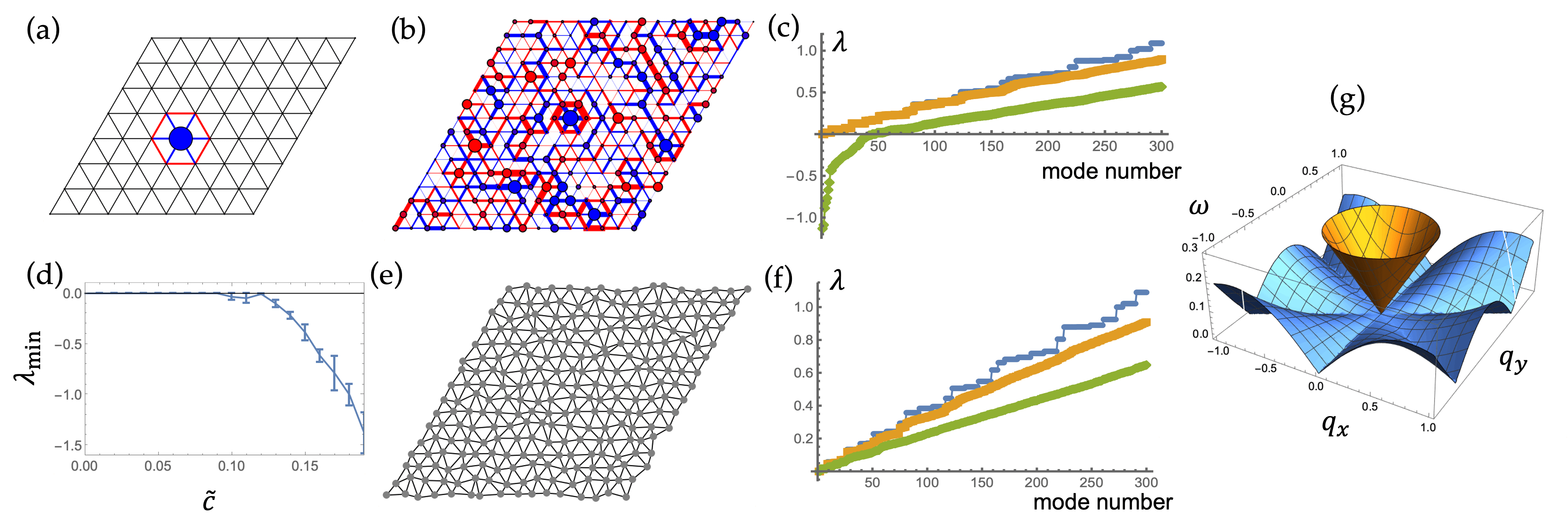
In particular, we can generate an ensemble of prestress on triangular lattices by taking an arbitrary coefficient for each site-localized SSS and sum them up. In Fig 5b we show an example of such a prestressed state.
These prestressed lattices can be physically constructed by choosing the rest length of each bond such that when they are at the length in the regular triangular lattice, the tension/compression they carry is exactly the value in the prescribed SSSs. Because the total force is balanced at each site for any SSS, all bonds will stay at the length in the regular lattice, and thus we obtain a triangular lattice with regular geometry and a prescribed SSS.
What are the mechanical properties of such prestressed triangular lattices? Here we study them from two perspectives: vibrational modes and load-bearing capabilities. The vibrational modes can be calculated based on the quadratic expansion in Eq. (3) for each bond, which leads to the dynamical matrix defined in Eq. (24).
In Fig. 5c we show eigenvalues of the dynamical matrix of the triangular lattice at three levels of prestress (by assigning from a Gaussian distribution with mean at and standard deviation at ). Prestress significantly affects the vibrational modes especially at low frequencies. In particular, negative eigenvalues start to appear when the fluctuations of the SSSs goes beyond a critical level, (Fig. 5c,d). This indicates that by increasing the fluctuation of prestress (where the mean remains 0), unstable modes appear, although the system remains in force balance. This is in alignment with our discussion on prestressed rigidity and type ZMs of prestressed systems in Sec. II.3.
To contrast this result, we also consider triangular lattices with positional disorder but no prestress (Fig. 5e). In this case, we move site by a random displacement , the components of which being generated from a Gaussian distribution with mean at and standard deviation at . We also plot the eigenvalues of the dynamical matrix of this case in Fig. 5f. Although positional disorder also affects the eigenvalues, it mostly smooths out the regular lattice eigenmodes, and does not lead to qualitative change at low frequencies and does not generate unstable modes. Note that to make a fair comparison we chose the same values for and , which represents the same level of disorder, under the simple convention we took where the bond length and spring constant on the triangular lattice both being unity.
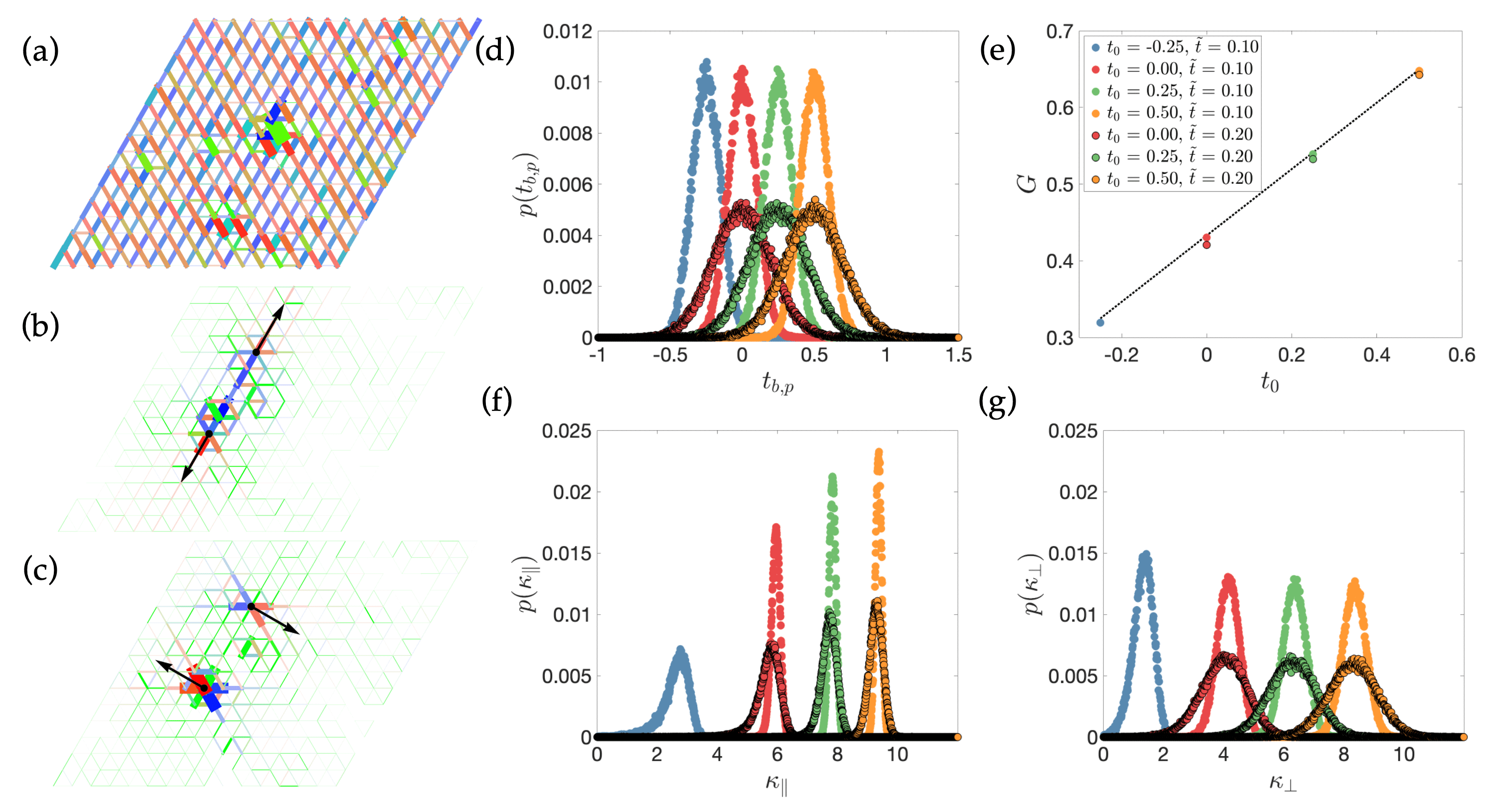
The load-bearing capabilities of prestressed triangular lattices can be analyzed by the SSSs formalism discussed in Sec. III. At any given realization of disordered prestress, we can compute the linear space of SSSs, and use Eq. (36) and (40) to find the stress response of the system to external load (Fig. 6a-c). In particular, to characterize the homogeneous component of prestress (hydrostatic pressure), we also introduce a constant pretension on all bonds, in addition to the fluctuations from . As a result, the tension on each bond obeys a normal distribution with mean at and standard deviation at (as each bond appears in 4 site-localized SSSs around it), as shown in Fig. 6d. We apply two types of load, simple shear and dipole forces, on these prestressed triangular lattices, and the results are shown in Fig. 6. This analysis shows that for both shear modulus and stiffness against dipole forces, their mean is mainly controlled by (where compression decreases stiffness and tension increases stiffness) whereas slightly decreases these stiffness, as well as broadens them. In addition, the stress response demonstrates interesting heterogeneities due to the disordered prestress, an effect we will discuss more in Sec. V.
Effects of prestress on mechanics can also be seen from the perspective of phonon structures of regular lattices (Figs. 2c and 5g). It is straightforward to see that negative prestress (compression) destabilizes the originally stable triangular lattice (Fig. 5g), and positive prestress (tension) stabilizes the honeycomb lattice (Fig. 2c), which was originally unstable against shear. Interestingly, the modes that first become unstable in the triangular lattice as negative prestress increase are the modes along the direction in the first Brillouin zone, indicating that the type of modes that first become unstable are the modes that zig-zag between the straight lines of bonds, agreeing with recent studies of strain-localization in lattice models Bordiga et al. 2021.
V Prestressed elasticity of amorphous solids of soft repulsive particles
The new matrix approach described in Sec. III provides a set of tools to analyze stress-bearing capabilities and mode structures of prestressed systems, well beyond the triangular lattices just described. Here we apply this method to a computational model for amorphous solids composed of soft repulsive particles, where, akin to real materials, prestresses are naturally introduced by the preparation (solidification) protocol. Given the preparation protocol chosen for this study, the prestress is the result of both compression and frozen-in structural disorder.
V.1 3D numerical simulations of amorphous solids of soft repulsive particles
The numerical model describes a suspension of particles with soft repulsive interactions given by a truncated and shifted Lennard-Jones potential Weeks et al. 1971. The potential energy, for a pair of two particles and separated by a center-to-center distance , is for particle pairs closer than the cutoff distance , otherwise , following the notation we defined in Sec. II. Here with and being the diameters. The size poly-dispersity is introduced by drawing the diameter of each particle from a Gaussian distribution with mean and variance of . The parameter is the unit energy and is the unit length in the simulations. Particles closer than the cutoff distance (beyond which the inter-particle force vanishes), , are considered in contact. All simulations used here have volume fraction and consist of particles in a cubic box of linear size , unless otherwise specified. The initial samples are prepared by first melting face-centered-cubic (FCC) crystals of particle at volume fraction at . We then cool the particle assemblies down to a temperature through an NVT molecular dynamics (MD) protocol as described in Ref. Vasisht and Del Gado 2020. The cooling rate varies from to , where is the MD time unit with the particle mass. Subsequently, each sample is brought to the closest local energy minimum using a conjugate gradient (CG) algorithm. The configurations prepared in this way are amorphous solids, as we verify by measuring their viscoelastic response Vasisht and Del Gado 2020, whose properties depend on the cooling rate utilized. These solids feature prestress that comes both from the homogeneous compression and from the structural disorder due to the size polydispersity.
From all contacting particle pairs, we compute the virial stress tensor Irving and Kirkwood 1950 (neglecting the kinetic term):
| (43) |
where is the volume of the system, is the distance between particle and (length of bond ), and is the force on bond .
In Fig. 7 we show a typical configuration where prestress on the bonds are visualized. These terms are negative as the system is compressed. For each cooling rate, we prepare 5 statistically independent samples. All quantities investigated here have been averaged over this set of samples and we obtain error bars from sample to sample fluctuations.
We also examine these samples as they are sheared using Lees-Edwards boundary conditions and a shear rate , by solving Newton equations of motions with a drag force that guarantees minimal inertia effects as discussed in Vasisht and Del Gado 2020. All simulations are performed with LAMMPS Plimpton 1995, suitably modified to include the particle size polydispersity and the interactions discussed above, and using a shear rate .
With the bond network and particle coordinates, we build the compatibility and equilibrium matrices and , to study the prestressed elasticity using the general formalism described in the previous sections. In this 3D network, each bond has one longitudinal and two transverse directions for tension increments. We take the convention that the first transverse direction is the unit vector of the cross product between the bond unit vector and the -axis , and the second transverse direction is the unit vector of the cross product between the bond vector and the first transverse direction [the subscript signifies the reference (undeformed but prestressed) state].

Once the and matrices are constructed, we solve their null space and obtain ZMs and SSSs of the computational model. The samples we studied are in general deep in the solid phase and exhibit no ZMs besides the 3 trivial translations. When solving for SSSs in large and dense systems as the samples we generated, the null space for the equilibrium matrix may have very high dimensions. We used the SPQR_RANK package Foster and Davis 2013 from SuiteSparse sui, which is a high performance sparse QR decomposition package and can provide a reliable determination of null space basis vectors for large sparse matrices, to solve for SSSs efficiently and reliably, especially when there are lots of degeneracies for diagonalizing . Similarly, SPQR_RANK is also suitable when solving for the null space of to get ZMs in large systems.
V.2 Calculating stress response to shear using states of self-stress
We begin by demonstrating the power of the SSSs as “stress-eigenstates” that characterize the stress-bearing capabilities of a system. To this end, we compute all SSSs as described above, and use Eq. (36) to calculate the change of tension, and , as the system is under macroscopic shear, which we call “prestressed response” here, as this is the difference between the stress under load and the prestress.
To contrast this result, we also calculated the tension increment treating the system as a stress-free network, i.e., as characterized by equilibrium matrix instead of (where the geometry of the contact network is kept the same). The resulting stress increment (which only has the component) is then calculated using Eq. (35), and we will call this the “stress-free response”. At the same time, we also measure the change of the stress in the system in a numerical experiment where the system is under a small shear deformation imposed quasistatic or at finite rate (as specified in captions of Figs. 8 and 9), and we call this the “actual response”.
In the next two subsections we compare these different results on tension increment in terms of both spatial heterogeneity and shear modulus.
V.3 Spatial heterogeneity of stress response

One significant effect of prestress on the mechanical response of amorphous solids is the spatial heterogeneity of the stress increment, in contrast to the stress-free response (where the geometry is kept the same). Fig. 8 shows a visualization of the tension increment in the model amorphous solids we study here.
Remarkably, this heterogeneity is accurately depicted from the SSSs calculation when prestress is included. The tension increment is computed following Eq. (36). The resulting field includes both and , although only is shown. To be precise, manifests as rotations of the bonds in the real response (which causes the total tension to change direction). In contrast, the calculated stress response of the system ignoring the prestress effect, i.e., using Eq. (35), is almost completely homogeneous. Thus, in these dense systems, the prestress controls the spatial heterogeneity of the mechanical response of the system. Treating the system as “stress-free” misses important signatures of heterogeneities.
We characterize the spatial heterogeneity of the tension increment using a clustering tendency index: the Hopkins statistic Hopkins and Skellam 1954, with a value close to 1 indicating the data is highly clustered, and a value around 0.5 from random data. Fig. 8(c) shows that the prestressed elasticity captures the tension increment clustering tendency which exists in real tension responses, while in stress-free elasticity this clustering is not captured.
V.4 Shear modulus of prestressed amorphous solids
The shear modulus can be obtained from the shear component of the virial stress. All the contributions to the virial stress in Eq. (43) can be obtained from the SSSs projection calculation (which directly gives of all bonds ) via
| (44) | ||||
| (45) |
where is the direction of the bond after the deformation. Comparing with the continuum limit we discussed at Eq. (II.2), this virial stress tensor is both a spatial average over the whole system, and uses the bond directions after deformation (which is along the calculated ) instead of original directions . In the terminology of structural mechanics, this virial stress [Eq. (43)] is the Cauchy stress (true stress, in the thermodynamic limit), and Eq. (II.2) defines the Second Piola-Kirchhoff stress which uses bond directions in the undeformed state. [In practice, using Eq. (II.2) would just result in slightly higher errors.]
In Fig. 9 we show the agreement between the actual and the calculated tension increment using the prestressed formulation on the bonds, as well as the agreement of the shear modulus. In contrast, the tension increment calculated from the stress-free formulation displays clear deviations.
This effect can also be viewed from the continuum elasticity formulation in Sec. II.2: when the macroscopic shear deformation field is plugged into the continuum theory, the elastic energy density is
| (46) |
leading to a prestress-corrected shear modulus of . It is straightforward from this relation that an isotropic compressional prestress () decreases the shear rigidity of a network.
The results shown so far demonstrates that including prestress effects is important to characterize the mechanical response of the model amorphous solids obtained from the simulations. We next use the configurations of the model amorphous solids to collect statistical information on the SSSs when different preparation protocols, i.e. different cooling rates, are utilized.

V.5 General statistics of states of self-stress
By varying the cooling rate as described above, we prepare particle assemblies that have different amount of disorder and compressive prestress, and have shown elsewhere that the higher cooling rates lead to a higher degree of disorder, characterized through a Voronoi analysis of the local particle packing which shows a decrease in the local icosahedral order Vasisht et al. 2020; Vasisht and Del Gado 2020.
The total number of SSSs in a prestressed system is directly related to the numbers of degrees of freedom and constraints via the Maxwell-Calladine index theorem [Eq. (30)] as the system exhibits no ZMs except for the trivial translations. In Fig. 10(a) we show the total number of SSSs in different configurations of our model amorphous solid that were prepared by varying the cooling rate. The number decreases with the increase of cooling rate. Figs. 10(b)-(d) show that this effect is accompanied by a decrease in the number of bonds and a decrease of the shear modulus, which is also associated to a net increase of the average compressional prestress. These findings support the idea that varying the preparation protocol by varying the cooling rate, as we do, induces different amount of prestress into amorphous solid configurations, which can be directly captured by the SSSs analysis. The data also indicate that more aged samples, which tend to be stiffer, feature larger amounts of SSSs. This is consistent with the finding in Ref. Vasisht et al. 2020 that more aged samples (i.e., prepared with a lower cooling rate) contained larger amounts of (overconstrained) icosahedrally packed domains, identified through the Voronoi analysis of the particle packing. These domains, which tend to be stiffer, were shown to favor the accumulation of stress and promote dilation when the samples were driven towards yielding under a shear deformation. The comparison of the results obtained here with the analysis performed in Refs. Vasisht et al. 2020; Vasisht and Del Gado 2020 support the idea that those phenomena, i.e., the increase in stiffness and in the tendency to accumulate stress and dilate under shear, should be due to prestress, and that sizable changes in the number of SSSs, as a result of sizable differences in prestress, eventually determine sizable changes in the linear, and even nonlinear, response of amorphous solids.

V.6 Dipole stiffness in prestressed glasses
SSSs have been also discussed in the context of the mechanical response of amorphous solids to local perturbations (e.g., force dipoles), which could be connected to the localized or quasi-localized plastic processes that are key ingredients of the mechanical response of this class of materials Sussman et al. 2016; Lerner 2018. The analysis of nonaffine and plastic microscopic displacements under shear and of their spatial correlations has led to the notion of “soft spot”, i.e., the presence of localized regions that are especially susceptible to plastic rearrangements under an external forceTanguy et al. 2002b; Leonforte et al. 2004; Maloney and Lemaître 2006; Chen et al. 2011; Schoenholz et al. 2014.

The local response to force dipoles that we have discussed in Sec. III.5 has been directly related to these soft spots in amorphous solids Sussman et al. 2016; Lerner 2018; Rainone et al. 2020b and such response analysis has pointed to quasilocalized excitations (QLEs). In general, one needs to follow the time evolution of a system under an external deformation to identify the QLEs, however similar characteristics have been extracted, in the case of model glasses and amorphous solids, even from the low-frequency limit of the vibrational spectrum, i.e., from the linear response regime Tanguy et al. 2002b; Chen et al. 2011; Schoenholz et al. 2014; Mosayebi et al. 2014.
Here we use the newly developed methods to examine the response of the model amorphous solids obtained in simulations to dipole forces, and collect the statistics of the local stiffness these systems display. In particular, we apply the approach for force dipoles discussed in Sec. III.5, and calculate the stiffness as defined in Eq. (41) for each bond, to identify regions which are soft. Measures of this kind lend themselves, in fact, to identify soft regions with respect to various external perturbations.
Interestingly, the relative displacement that a pair of particles undergoes during a plastic rearrangement is typically not along the direction of the bond that initially connects them. Instead, this local deformation involves several sliding motions. Therefore, a particularly interesting measure of local softness, potentially complementing recently proposed ones Lerner 2018; Cubuk et al. 2015; Richard et al. 2020, can be obtained by quantifying the stiffness against a dipole, whose forces are along a different direction from the one of the bond on which they are applied. Thus, for each bond, in addition to computing the dipole stiffness to longitudinal (along ) and transverse (along ) forces, we compute the softest dipole stiffness, , by minimizing it with respect to the direction of the dipole forces (details in App. B).
Fig. 11(a) shows an example of applying longitudinal and transverse force dipoles on a bond in our prestressed particle configurations, showing both and tension responses of all bonds. Remarkably, although the near field response is mainly in the direction, the far field response contains significant components. This is a genuine effect of prestress—these transverse stress response can only be captured when prestress is included.
We collect the statistics of the minimum dipole stiffness on bonds in the networks obtained with two different preparation cooling rates as shown in Fig. 11(g). These distributions feature a power-law tail for small , where and appears to depend on the cooling rate. The results demonstrate the impact of preparation history to the mechanical stiffness in prestressed systems. The case with faster cooling rate leads to a smaller exponent and thus the distribution extends more to soft , agreeing with the general trend discussed in Sec. V.5, where faster cooling rate leaves more heterogeneities regarding stress response in the sample. Our results also provide an interesting comparison to (longitudinal) dipole stiffness distributions studied in Ref. Rainone et al. 2020a for different models of computational glasses.
Furthermore, we also characterize the spatial distribution of and compare it to the spatial distribution of prestress (Fig. 11h,i). Remarkably, shows interesting spatial patterns whose possible correlations with the amount of prestress in these regions are however hard to tease out. Relating regions with clustered soft with soft spots will be an interesting question for future studies.
VI Discussion
Through this paper, we have developed a set of mathematical tools to investigate elasticity of prestressed discrete networks, which allows to disentangle the prestress from the structural disorder, offering new insight into the mechanical response of amorphous solids.
Our theory is based on the equilibrium and compatibility matrices, which rigorously defines SSSs and ZMs in mechanical networks. SSSs provide a linear space for the ensemble of force-balanced prestress distributions of the network, therefore capturing the possibility that the prestress may vary without altering the network configuration. Any mechanical network with SSSs can become prestressed, e.g., by introducing mismatching bond lengths (geometric frustration), which naturally arises in the solidification of amorphous solids in general. These We have generalized the equilibrium and compatibility matrices to these prestressed systems, which amounts to include additional constraints on bonds from prestress. We have then used the new mathematical tools to analyze the mechanical response of prestressed triangular lattices and model amorphous solids obtained through 3D numerical simulations, and found good agreement between the numerically measured response and results obtained from our methods, whereas the time-complexity of the computation is greatly reduced.
In particular, we not only characterize how prestress affects vibrational modes, both stabilizing soft modes and introducing a new class of ZMs (type , which appear due to competing positive and negative terms in the energy), but also reveal its profound role on how the network carries additional stress. By analyzing prestressed SSSs of the network, and projecting external load to this linear space, our methods conveniently map how external stress transmits in prestressed lattices and bond networks obtained from model amorphous solids. We show a number of intriguing effects which are unique to prestressed networks, including the spatial heterogeneity in the stress-response to homogeneous loads, the power-law distribution of the local stiffness and the isotropic nature of the long-range stress response to local perturbations such as force dipoles.
These results provide new tools and insight to unravel the complexity of mechanical properties of amorphous solids. They also open new paths for further exploration. For example, the new measure of minimum dipole stiffness we propose is potentially a new direct probe to analyze soft spots in amorphous solids. Relating this measure with existing characterizations of soft spots, as well as yielding of amorphous solids, will be interesting topics for future studies.
Moreover, the ability to separately vary the prestress and the microscopic bond configuration in our theory offers a new perspective to analyze the dynamics of amorphous solids under strain. In real amorphous solids, from granular matter to colloids, particle-particle interactions are not simple harmonic springs. Instead, they evolve under stress in complicated and often unpredictable ways—micro-fracturing, crushing, sintering. This evolution is further complicated by the role of the solvent, where contacts between particles can be lubricated or frictional. Therefore, stress distributions can significantly change with little change in the configuration. Our methods provide a convenient set of tools to examine how the mechanical response of these amorphous materials may evolve as the system explores an ensemble of states where only internal stress is changed.
Prestress records the preparation history in amorphous solids and has an important role in directing the mechanical response beyond the linear regime. The implications of prestress and preparation history, in fact, have been highlighted with respect to the development of flow inhomogeneities upon yielding Vasisht et al. 2020 and in connection with the fundamental physics mechanisms controlling brittle or ductile yielding phenomena Ozawa et al. 2018; Singh et al. 2020; Barlow et al. 2020. Our methods, therefore, have wider relevance as they can be applied beyond the linear response to investigate, through the SSSs characteristics, the role of prestress in plasticity and yielding. The new tools discussed here can potentially close the feedback loop between structure and stress, opening a new pathway to study how amorphous solids yield and solidify under external strain.
Finally, friction plays a central role in the complex behaviors of exotic rigid states emerging in granular matter and dense suspensions, leading to fascinating phenomena from shear jamming to discontinuous shear thickening Bi et al. 2011; Seto et al. 2013; Wyart and Cates 2014; Lin et al. 2016; Guy et al. 2018; Liu et al. 2021b; Ramaswamy et al. 2021. Interestingly, friction also lives in the channel of stress, and a linear relation with can also be assumed, hence it would be a natural next step to include friction into the SSSs description. However, the Coulomb threshold imposes an upper limit to that is not part of the methods developed here. How the frictional and the prestress contributions to interplay and affect the macroscopic dynamics of the material, will be of great interest for future studies.
Acknowledgements.
This work is supported in part by the National Science Foundation under grant number NSF-DMR-2026825 (E.D.G and X.M.), NSF-EFRI-1741618 (S.Z., L.Z., and X.M.), and the Office of Naval Research under grant number MURI N00014-20-1-2479 (E.S. and X.M.)Appendix A SSSs formulation for shear response of prestressed networks
A.1 Projection of a shear load to the SSSs linear space
When a mechanical network is subject to a shear load, the resulting bond extensions and rotations can be written as the sum of contributions from the affine shear field and the nonaffine displacements ,
| (47) |
which is similar to Eq. (33) in the main text, but here we include both the parallel and the perpendicular components of .
When force-balance is reached, net force on each particle vanishes,
| (48) |
This means that must be a vector that belongs to the null space of . Thus it can be written as a linear combinations of the SSSs of the system.
To facilitate the discussion of this SSSs linear combination, we define the following notations. Let be an orthonormal basis of the null space of , and let denote the matrix whose columns are , i.e., . One can also define the dimensional matrix whose columns are an orthonormal basis of the orthogonal compliment of the null space of . Similarly one can define the matrix whose columns are an orthonormal basis of the null space of (ZMs), and the matrix whose columns are an orthonormal basis of the orthogonal compliment of the null space of . These matrices are represented as,
| (49) | ||||
| (50) | ||||
| (51) | ||||
| (52) |
and they satisfy the following identities,
| (53) | ||||
| (54) | ||||
| (55) | ||||
| (56) | ||||
| (57) | ||||
| (58) |
where is an identity matrix of dimension , and other definitions follows similarly.
As we discussed above, is a linear combination of the SSSs,
| (59) |
where are coefficients of the linear combination of as the SSSs.
Because the basis we use are orthonormal,
| (60) | ||||
| (61) |
inserting identity matrix [Eq. (57)] into Eq. (61) and using the fact that,
we have,
| (62) |
where we defined the decomposition of into the null and orthogonal compliment space as
| (63) |
and also used the fact that is invertible.
This can be further simplified by letting , and decompose into the column-space and null-space of as,
| (65) |
One can see that,
| (66) | ||||
| (67) |
Right multiply by on both sides of two equations,
| (68) | |||
| (69) |
Then,
| (70) | |||
| (71) |
Combining these two equations we have,
| (72) | ||||
| (73) |
As a result, is simplified to
| (74) |
and the tension response to this external shear is
| (75) |
Note that this includes both and , and this formulation applies to other types of homogeneous strain, such as hydrostatic compression, as well.
A.2 Affine bond deformation in prestressed systems
In this subsection we derive the field for any external load represented by a strain tensor .
Appendix B Dipole stiffness in prestressed systems
When a pair of dipole forces is applied on a mechanical network between two particles that belong to the same rigid cluster, the network will show a linear response with tension distributed on the bonds. In this Appendix we derive the stress field of a prestressed network in response to the force dipole, and obtain a computationally efficient formula that gives the stiffness the system has against this force dipole.
B.1 Local dipole stiffness
As discussed in Sec. III.5, the sum of the external force dipole and the tension response, , must be a SSS of the prestressed network,
The coefficients are determined in the same way as discussed in App. A, just by replacing with . As a result
We can thus use this in the expression for the dipole stiffness [Eq. (41)], where the denominator is now
| (78) |
where we used Eq. (38) and the fact that (bond extension causes tension).
Therefore the dipole stiffness is
| (79) | ||||
where the factor of 2 in the last line comes from the fact that involves 2 particles.
B.2 Non-local dipole stiffness
Besides applying the force dipole on an arbitrary existing bond in the system, one could also apply a force dipole between two particles which are not connected. As we discuss below, this pair of dipole introduces a new constraint into the system.
Force balance with imposed force dipole can be written as:
| (80) |
where indicates the particle displacements in response to the force dipole as the system reaches force balance. Unlike the local dipole case discussed above, here can not be written as on an existing bond, as the two sites are not connected. Instead, we can introduce an auxiliary bond between the two sites that carry . In this sense, a new constraint and thus a new SSS is added to the system by the auxiliary bond.
Here we introduce the new matrices after introducing the auxiliary bond (which has zero spring constant so that it will not induce tension responses) as
The dimension of the bond space is extended with one additional component from the auxiliary bond indexed as .
Now the force-balanced total tension can be written as
| (81) |
where lives on the auxillary bond. This satisfies force balance and must be a SSS of the network with the auxillary bond.
Similar to App. A, one can define to the new matrices. We can then decompose the total tension onto SSSs,
where ’s are coefficients of the linear combination of the SSSs.
We can compute the tension in a similar way,
Thus
| (82) | ||||
| (83) | ||||
| (84) | ||||
| (85) |
As a result,
| (86) |
Note that although the spring constant of the auxiliary bond is 0, the matrix is still invertable. This is because the auxiliary bond is a redundant bond (otherwise the network would yield, resulting in no stress in linear response), which increases the dimension of the SSSs space and does not introduce new vectors in the orthogonal compliment space. As a result, and is invertable.
This can be used to find the coefficients for the SSSs
| (87) |
where in the last line we used Eq. (86). These coefficients gives the tension field in response to a nonlocal dipole.
We can then proceed to calculate the dipole stiffness. Applying on both sides of Eq. (86), we have the left hand side,
| (88) | ||||
| (89) | ||||
| (90) |
Equaling it to the right hand side we have
| (91) |
expressing the displacement field as a function of the imposed dipole.
One can then compute the non-local dipole stiffness as (the force dipole where is the vector in the labeling space of bonds which has zeros in all bonds and unity on the -th component (the auxiliary bond), and a spring constant of unity is added (which is only used to represent the external force dipole, where the actual spring constant of the auxillary bond regarding its contribution to the network response is still 0 as discussed above),
| (92) | ||||
| (93) | ||||
| (94) | ||||
| (95) | ||||
| (96) |
The local force dipole response is a special case of non-local force dipole response. When considering local force dipoles, the auxiliary bond overlaps with bond . One can show that in this case, the non-local force dipole stiffness reduces to local force dipole stiffness.
B.3 Minimum local dipole stiffness in prestressed systems
In this section we derive the minimum dipole stiffness on any given bond , which is the lowest with respect to the combination of and directions. To do this we use to denote the direction of the dipole forces, and the resulting can be written as
| (97) |
where we defined the new vector for this case allowing arbitrary force directions. We can plug this in Eq. (79) to find the dipole stiffness for any given , and represent the nontrivial term in as
| (98) | ||||
| (99) | ||||
| (100) |
where represents the matrix in between vectors in Eq. (98) and is the part of associated with bond .
Similarly,
where and are the parts of and associated with bond , respectively.
As a result,
Minimizing for a single bond ,
| (101) |
is an optimization problem with respect to the two variables and . To solve for such optimization problems in our system, we used the Nelder-Mead simplex algorithm as described in Ref. Lagarias et al. 1998.
By doing this minimization, we obtain as the softest dipole stiffness direction for any bond , which is typically transverse.
References
- Alexander (1998) S. Alexander, Physics reports 296, 65 (1998).
- Ulm and Coussy (2003) F.-J. Ulm and O. Coussy, Mechanics and Durability of Solids. Solid mechanics (Pearson Education, 2003).
- Wyart et al. (2005) M. Wyart, L. E. Silbert, S. R. Nagel, and T. A. Witten, Phys. Rev. E 72, 051306 (2005).
- Bouzid et al. (2017) M. Bouzid, J. Colombo, L. V. Barbosa, and E. Del Gado, Nature Communications 8, 15846 (2017).
- Bi et al. (2011) D. Bi, J. Zhang, B. Chakraborty, and R. P. Behringer, Nature 480, 355–358 (2011).
- Sehgal et al. (2019) P. Sehgal, M. Ramaswamy, I. Cohen, and B. J. Kirby, Phys. Rev. Lett. 123, 128001 (2019).
- Ballauff et al. (2013) M. Ballauff, J. M. Brader, S. U. Egelhaaf, M. Fuchs, J. Horbach, N. Koumakis, M. Krüger, M. Laurati, K. J. Mutch, G. Petekidis, M. Siebenbürger, T. Voigtmann, and J. Zausch, Phys. Rev. Lett. 110, 215701 (2013).
- Gei et al. (2009) M. Gei, A. B. Movchan, and D. Bigoni, Journal of Applied Physics 105, 063507 (2009), https://doi.org/10.1063/1.3093694 .
- Chen et al. (2012) Z. Chen, Q. Guo, C. Majidi, W. Chen, D. J. Srolovitz, and M. P. Haataja, Phys. Rev. Lett. 109, 114302 (2012).
- Fraternali et al. (2014) F. Fraternali, G. Carpentieri, A. Amendola, R. E. Skelton, and V. F. Nesterenko, Applied Physics Letters 105, 201903 (2014), https://doi.org/10.1063/1.4902071 .
- Meeussen et al. (2020) A. S. Meeussen, E. C. Oğuz, M. van Hecke, and Y. Shokef, New Journal of Physics 22, 023030 (2020).
- Merrigan et al. (2021) C. Merrigan, C. Nisoli, and Y. Shokef, Phys. Rev. Research 3, 023174 (2021).
- Armon et al. (2011) S. Armon, E. Efrati, R. Kupferman, and E. Sharon, Science 333, 1726 (2011), https://science.sciencemag.org/content/333/6050/1726.full.pdf .
- Wyczalkowski et al. (2012) M. A. Wyczalkowski, Z. Chen, B. A. Filas, V. D. Varner, and L. A. Taber, Birth Defects Research Part C: Embryo Today: Reviews 96, 132 (2012), https://onlinelibrary.wiley.com/doi/pdf/10.1002/bdrc.21013 .
- Feng et al. (2018) D. Feng, J. Notbohm, A. Benjamin, S. He, M. Wang, L.-H. Ang, M. Bantawa, M. Bouzid, E. Del Gado, R. Krishnan, and M. R. Pollak, Proceedings of National Academy of Sciences 115, 1517 (2018).
- Zhang et al. (2017) L. Zhang, D. Z. Rocklin, L. M. Sander, and X. Mao, Physical Review Materials 1, 052602 (2017).
- Ozawa et al. (2018) M. Ozawa, L. Berthier, G. Biroli, A. Rosso, and G. Tarjus, Proceedings of the National Academy of Sciences 115, 6656 (2018), https://www.pnas.org/content/115/26/6656.full.pdf .
- Vasisht et al. (2020) V. V. Vasisht, G. Roberts, and E. Del Gado, Physical Review E 102, 010604 (2020).
- Barlow et al. (2020) H. J. Barlow, J. O. Cochran, and S. M. Fielding, Phys. Rev. Lett. 125, 168003 (2020).
- Berthier et al. (2019) E. Berthier, J. E. Kollmer, S. E. Henkes, K. Liu, J. M. Schwarz, and K. E. Daniels, Phys. Rev. Materials 3, 075602 (2019).
- Debenedetti and Stillinger (2001) P. G. Debenedetti and F. H. Stillinger, Nature 410, 259 (2001).
- Manning and Liu (2011) M. L. Manning and A. J. Liu, Phys. Rev. Lett. 107, 108302 (2011).
- Ninarello et al. (2017) A. Ninarello, L. Berthier, and D. Coslovich, Phys. Rev. X 7, 021039 (2017).
- Vasisht et al. (2021) V. V. Vasisht, P. Chaudhuri, and K. Martens, “Residual stress in athermal soft disordered solids: insights from microscopic and mesoscale models,” (2021), arXiv:2108.12782 [cond-mat.soft] .
- Bhaumik et al. (2021) H. Bhaumik, G. Foffi, and S. Sastry, Proceedings of the National Academy of Sciences 118 (2021), 10.1073/pnas.2100227118.
- Richard et al. (2020) D. Richard, M. Ozawa, S. Patinet, E. Stanifer, B. Shang, S. A. Ridout, B. Xu, G. Zhang, P. K. Morse, J.-L. Barrat, L. Berthier, M. L. Falk, P. Guan, A. J. Liu, K. Martens, S. Sastry, D. Vandembroucq, E. Lerner, and M. L. Manning, Phys. Rev. Materials 4, 113609 (2020).
- Bouchaud (2002) J.-P. Bouchaud, arXiv preprint cond-mat/0211196 (2002).
- Aben et al. (2016) H. Aben, J. Anton, M. Õis, K. Viswanathan, S. Chandrasekar, and M. M. Chaudhri, Applied Physics Letters 109, 231903 (2016), https://doi.org/10.1063/1.4971339 .
- Wen et al. (2020) L. Wen, F. Pan, and X. Ding, Science Robotics 5, eabd9158 (2020).
- DeGiuli et al. (2014) E. DeGiuli, A. Laversanne-Finot, G. Düring, E. Lerner, and M. Wyart, Soft Matter 10, 5628 (2014).
- Ellenbroek et al. (2009) W. G. Ellenbroek, M. van Hecke, and W. van Saarloos, Phys. Rev. E 80, 061307 (2009).
- Licup et al. (2015) A. J. Licup, S. Münster, A. Sharma, M. Sheinman, L. M. Jawerth, B. Fabry, D. A. Weitz, and F. C. MacKintosh, Proceedings of the National Academy of Sciences 112, 9573 (2015), https://www.pnas.org/content/112/31/9573.full.pdf .
- Feng et al. (2015) J. Feng, H. Levine, X. Mao, and L. M. Sander, Physical Review E 91, 042710 (2015).
- Feng et al. (2016) J. Feng, H. Levine, X. Mao, and L. M. Sander, Soft matter 12, 1419 (2016).
- Noll et al. (2017) N. Noll, M. Mani, I. Heemskerk, S. J. Streichan, and B. I. Shraiman, Nature physics 13, 1221 (2017).
- Hardin et al. (2018) C. Hardin, J. Chattoraj, G. Manomohan, J. Colombo, T. Nguyen, D. Tambe, J. J. Fredberg, J. P. Birukov, K. Butler, E. Del Gado, and R. Krishnan, Biochem Biophys Res Commun 495, 749 (2018).
- Yan and Bi (2019) L. Yan and D. Bi, Phys. Rev. X 9, 011029 (2019).
- Merkel et al. (2019) M. Merkel, K. Baumgarten, B. P. Tighe, and M. L. Manning, Proceedings of the National Academy of Sciences 116, 6560 (2019).
- Liu et al. (2021a) H. Liu, D. Zhou, L. Zhang, D. K. Lubensky, and X. Mao, arXiv preprint arXiv:2104.14743 (2021a).
- Alvarado et al. (2013) J. Alvarado, M. Sheinman, A. Sharma, F. C. MacKintosh, and G. H. Koenderink, Nature Physics 9, 591 (2013).
- Ronceray et al. (2016) P. Ronceray, C. P. Broedersz, and M. Lenz, Proceedings of the national academy of sciences 113, 2827 (2016).
- Tanguy et al. (2002a) A. Tanguy, J. P. Wittmer, F. Leonforte, and J.-L. Barrat, Phys. Rev. B 66, 174205 (2002a).
- O’Hern et al. (2003) C. S. O’Hern, L. E. Silbert, A. J. Liu, and S. R. Nagel, Phys. Rev. E 68, 011306 (2003).
- Zaccone and Scossa-Romano (2011) A. Zaccone and E. Scossa-Romano, Phys. Rev. B 83, 184205 (2011).
- Liu and Nagel (2010) A. J. Liu and S. R. Nagel, Annu. Rev. Condens. Matter Phys. 1, 347 (2010).
- Snoeijer et al. (2004) J. H. Snoeijer, T. J. H. Vlugt, M. van Hecke, and W. van Saarloos, Phys. Rev. Lett. 92, 054302 (2004).
- Tighe et al. (2008) B. P. Tighe, A. R. T. van Eerd, and T. J. H. Vlugt, Phys. Rev. Lett. 100, 238001 (2008).
- Tighe et al. (2010) B. P. Tighe, J. H. Snoeijer, T. J. Vlugt, and M. van Hecke, Soft Matter 6, 2908 (2010).
- Bi et al. (2015) D. Bi, S. Henkes, K. E. Daniels, and B. Chakraborty, Annual Review of Condensed Matter Physics 6, 63 (2015), https://doi.org/10.1146/annurev-conmatphys-031214-014336 .
- Edwards and Oakeshott (1989) S. F. Edwards and R. Oakeshott, Physica A: Statistical Mechanics and its Applications 157, 1080 (1989).
- Mao et al. (2007) X. Mao, P. M. Goldbart, X. Xing, and A. Zippelius, Europhysics Letters (EPL) 80, 26004 (2007).
- Henkes and Chakraborty (2009) S. Henkes and B. Chakraborty, Phys. Rev. E 79, 061301 (2009).
- Mao et al. (2009) X. Mao, P. M. Goldbart, X. Xing, and A. Zippelius, Phys. Rev. E 80, 031140 (2009).
- Lemaître (2017) A. Lemaître, Phys. Rev. E 96, 052101 (2017).
- Maier et al. (2017) M. Maier, A. Zippelius, and M. Fuchs, Phys. Rev. Lett. 119, 265701 (2017).
- DeGiuli (2018) E. DeGiuli, Phys. Rev. Lett. 121, 118001 (2018).
- Nampoothiri et al. (2020) J. N. Nampoothiri, Y. Wang, K. Ramola, J. Zhang, S. Bhattacharjee, and B. Chakraborty, Phys. Rev. Lett. 125, 118002 (2020).
- Calladine (1978) C. R. Calladine, International journal of solids and structures 14, 161 (1978).
- Pellegrino and Calladine (1986) S. Pellegrino and C. R. Calladine, International Journal of Solids and Structures 22, 409 (1986).
- Sun et al. (2012) K. Sun, A. Souslov, X. Mao, and T. Lubensky, Proceedings of the National Academy of Sciences 109, 12369 (2012).
- Kane and Lubensky (2014) C. Kane and T. Lubensky, Nature Physics 10, 39 (2014).
- Lubensky et al. (2015) T. Lubensky, C. Kane, X. Mao, A. Souslov, and K. Sun, Reports on Progress in Physics 78, 073901 (2015).
- Mao and Lubensky (2018) X. Mao and T. C. Lubensky, Annual Review of Condensed Matter Physics 9, 413 (2018).
- Paulose et al. (2015) J. Paulose, A. S. Meeussen, and V. Vitelli, Proceedings of the National Academy of Sciences 112, 7639 (2015).
- Zhang and Mao (2018) L. Zhang and X. Mao, New Journal of Physics 20, 063034 (2018).
- Sussman et al. (2016) D. M. Sussman, C. P. Goodrich, and A. J. Liu, Soft matter 12, 3982 (2016).
- Wyart et al. (2008) M. Wyart, H. Liang, A. Kabla, and L. Mahadevan, Physical review letters 101, 215501 (2008).
- Chen et al. (2011) K. Chen, M. L. Manning, P. J. Yunker, W. G. Ellenbroek, Z. Zhang, A. J. Liu, and A. G. Yodh, Phys. Rev. Lett. 107, 108301 (2011).
- Lerner et al. (2012) E. Lerner, G. Düring, and M. Wyart, Proceedings of the National Academy of Sciences 109, 4798 (2012).
- Mosayebi et al. (2014) M. Mosayebi, P. Ilg, A. Widmer-Cooper, and E. Del Gado, Phys. Rev. Lett. 112, 105503 (2014).
- Stanifer et al. (2018) E. Stanifer, P. K. Morse, A. A. Middleton, and M. L. Manning, Phys. Rev. E 98, 042908 (2018).
- Born et al. (1955) M. Born, K. Huang, and M. Lax, American Journal of Physics 23, 474 (1955).
- DiDonna and Lubensky (2005) B. DiDonna and T. Lubensky, Physical Review E 72, 066619 (2005).
- Maxwell (1864) J. C. Maxwell, The London, Edinburgh, and Dublin Philosophical Magazine and Journal of Science 27, 294 (1864).
- Tay and Whiteley (1984) T.-S. Tay and W. Whiteley, Structural Topology, 1984, núm. 9 (1984).
- Jacobs and Thorpe (1995) D. J. Jacobs and M. F. Thorpe, Physical review letters 75, 4051 (1995).
- Connelly and Whiteley (1992) R. Connelly and W. Whiteley, International Journal of Space Structures 7, 153 (1992).
- Connelly and Whiteley (1996) R. Connelly and W. Whiteley, SIAM Journal on Discrete Mathematics 9, 453 (1996).
- Vermeulen et al. (2017) M. F. Vermeulen, A. Bose, C. Storm, and W. G. Ellenbroek, Physical Review E 96, 053003 (2017).
- Damavandi et al. (2021) O. K. Damavandi, V. F. Hagh, C. D. Santangelo, and M. L. Manning, arXiv preprint arXiv:2102.11310 (2021).
- Rocklin et al. (2017) D. Z. Rocklin, S. Zhou, K. Sun, and X. Mao, Nature communications 8, 1 (2017).
- Zhou et al. (2018) D. Zhou, L. Zhang, and X. Mao, Phys. Rev. Lett. 120, 068003 (2018).
- Ma et al. (2018) J. Ma, D. Zhou, K. Sun, X. Mao, and S. Gonella, Phys. Rev. Lett. 121, 094301 (2018).
- Zhou et al. (2019) D. Zhou, L. Zhang, and X. Mao, Phys. Rev. X 9, 021054 (2019).
- Zhou et al. (2020) D. Zhou, J. Ma, K. Sun, S. Gonella, and X. Mao, Phys. Rev. B 101, 104106 (2020).
- Sun and Mao (2020) K. Sun and X. Mao, Phys. Rev. Lett. 124, 207601 (2020).
- Lerner (2018) E. Lerner, The European Physical Journal E 41, 1 (2018).
- Rainone et al. (2020a) C. Rainone, E. Bouchbinder, and E. Lerner, The Journal of Chemical Physics 152, 194503 (2020a).
- Bordiga et al. (2021) G. Bordiga, L. Cabras, A. Piccolroaz, and D. Bigoni, Journal of the Mechanics and Physics of Solids 146, 104198 (2021).
- Weeks et al. (1971) J. D. Weeks, D. Chandler, and H. C. Andersen, The Journal of chemical physics 54, 5237 (1971).
- Vasisht and Del Gado (2020) V. V. Vasisht and E. Del Gado, Physical Review E 102, 012603 (2020).
- Irving and Kirkwood (1950) J. H. Irving and J. G. Kirkwood, The Journal of Chemical Physics 18, 817 (1950).
- Plimpton (1995) S. Plimpton, Journal of computational physics 117, 1 (1995).
- Foster and Davis (2013) L. V. Foster and T. A. Davis, ACM Transactions on Mathematical Software (TOMS) 40, 1 (2013).
- (95) https://people.engr.tamu.edu/davis/suitesparse.html.
- Hopkins and Skellam (1954) B. Hopkins and J. G. Skellam, Annals of Botany 18, 213 (1954).
- Tanguy et al. (2002b) A. Tanguy, J. P. Wittmer, F. Leonforte, and J.-L. Barrat, Phys. Rev. B 66, 174205 (2002b).
- Leonforte et al. (2004) F. Leonforte, A. Tanguy, J. P. Wittmer, and J.-L. Barrat, Phys. Rev. B 70, 014203 (2004).
- Maloney and Lemaître (2006) C. E. Maloney and A. Lemaître, Phys. Rev. E 74, 016118 (2006).
- Schoenholz et al. (2014) S. S. Schoenholz, A. J. Liu, R. A. Riggleman, and J. Rottler, Phys. Rev. X 4, 031014 (2014).
- Rainone et al. (2020b) C. Rainone, E. Bouchbinder, and E. Lerner, Proceedings of the National Academy of Sciences 117, 5228 (2020b).
- Cubuk et al. (2015) E. D. Cubuk, S. S. Schoenholz, J. M. Rieser, B. D. Malone, J. Rottler, D. J. Durian, E. Kaxiras, and A. J. Liu, Phys. Rev. Lett. 114, 108001 (2015).
- Singh et al. (2020) M. Singh, M. Ozawa, and L. Berthier, Phys. Rev. Materials 4, 025603 (2020).
- Seto et al. (2013) R. Seto, R. Mari, J. F. Morris, and M. M. Denn, Physical review letters 111, 218301 (2013).
- Wyart and Cates (2014) M. Wyart and M. E. Cates, Physical review letters 112, 098302 (2014).
- Lin et al. (2016) N. Y. Lin, C. Ness, M. E. Cates, J. Sun, and I. Cohen, Proceedings of the National Academy of Sciences 113, 10774 (2016), https://www.pnas.org/content/113/39/10774.full.pdf .
- Guy et al. (2018) B. M. Guy, J. A. Richards, D. J. M. Hodgson, E. Blanco, and W. C. K. Poon, Phys. Rev. Lett. 121, 128001 (2018).
- Liu et al. (2021b) K. Liu, J. E. Kollmer, K. E. Daniels, J. M. Schwarz, and S. Henkes, Phys. Rev. Lett. 126, 088002 (2021b).
- Ramaswamy et al. (2021) M. Ramaswamy, I. Griniasty, D. B. Liarte, A. Shetty, E. Katifori, E. Del Gado, J. P. Sethna, B. Chakraborty, and I. Cohen, arXiv preprint arXiv:2107.13338 (2021).
- Lagarias et al. (1998) J. C. Lagarias, J. A. Reeds, M. H. Wright, and P. E. Wright, SIAM Journal on optimization 9, 112 (1998).