Modelling wave propagation in elastic solids via high-order accurate implicit-mesh discontinuous Galerkin methods

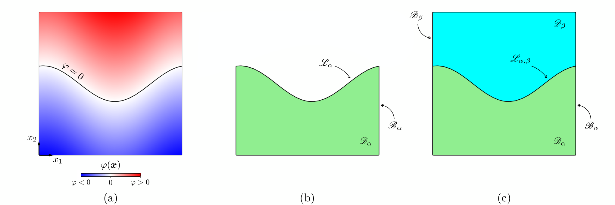
The geometry of a single-phase or a bi-phase solid is described implicitly by a level set function. Consider a $d$-dimensional rectangle $\mathscr{R}\subset\mathbb{R}^{d}$ and its outer boundary $\partial\mathscr{R}$. Consider also a level set function $\varphi:\mathscr{R}\rightarrow\mathbb{R}$ and let $\mathscr{R}^{-}\equiv\{\boldsymbol{x}\in\mathscr{R}:\varphi(\boldsymbol{x})<0\}$ be the portion of $\mathscr{R}$ where $\varphi$ is negative, $\mathscr{R}^{+}\equiv\{\boldsymbol{x}\in\mathscr{R}:\varphi(\boldsymbol{x})>0\}$ be the portion of $\mathscr{R}$ where $\varphi$ is positive and $\mathscr{L}\equiv\{\boldsymbol{x}\in\mathscr{R}:\varphi(\boldsymbol{x})=0\}$ be the zero-contour of $\varphi$. Moreover, let $\partial\mathscr{R}^{-}\equiv\{\boldsymbol{x}\in\partial\mathscr{R}:\varphi(\boldsymbol{x})<0\}$ be the portion of $\partial\mathscr{R}$ where $\varphi$ is negative and $\partial\mathscr{R}^{+}\equiv\{\boldsymbol{x}\in\partial\mathscr{R}:\varphi(\boldsymbol{x})>0\}$ be the portion of $\partial\mathscr{R}$ where $\varphi$ is positive.

Then, we define the domain $\mathscr{D}_{\alpha}$ and the boundary $\partial\mathscr{D}_{\alpha}$ of a solid consisting of one phase $\alpha$ as $\mathscr{D}_{\alpha}\equiv\mathscr{R}^{-}$ and $\partial\mathscr{D}_{\alpha}\equiv\mathscr{B}_{\alpha}\cup\mathscr{L}_{\alpha}$, respectively, where $\mathscr{B}_{\alpha}\equiv\partial\mathscr{R}^{-}$ and $\mathscr{L}_{\alpha}\equiv\mathscr{L}$. Alternatively, for a bi-phase solid consisting of two distinct phases $\alpha$ and $\beta$, we define the domain and the outer boundary of the phase $\alpha$ as $\mathscr{D}_{\alpha}\equiv\mathscr{R}^{-}$ and $\mathscr{B}_{\alpha}\equiv\partial\mathscr{R}^{-}$, respectively, the domain and the outer boundary of the phase $\beta$ as $\mathscr{D}_{\beta}\equiv\mathscr{R}^{+}$ and $\mathscr{B}_{\beta}\equiv\partial\mathscr{R}^{+}$, respectively, and the interface between the two phases as $\mathscr{L}_{\alpha,\beta}\equiv\mathscr{L}$.

As an example, Fig.(1a) shows a level set function $\varphi$ defined over a square, while Fig.(1b) shows the domain and the boundaries of the corresponding two-dimensional single-phase solid, and Fig.(1c) shows the domains, boundaries and interface of the corresponding two-dimensional bi-phase solid.

The governing equations of linear elastodynamics can be stated using different formulations, which, on the basis of the chosen set of primary variables, include the displacement formulation, see e.g. [9, 10], the velocity-stress formulation, see e.g. [37], or the momentum-strain formulation, see e.g. [39]. Here, we use the momentum-strain formulation since it allows for the consideration of materials with space-dependent constitutive properties. In the following, the governing equations, the initial conditions and the boundary conditions, are written for the domain $\mathscr{D}_{\alpha}$ and its boundary $\partial\mathscr{D}_{\alpha}$, but are also valid for the domain $\mathscr{D}_{\beta}$ and its boundary $\partial\mathscr{D}_{\beta}$, if one replaces the subscript $\alpha$ with $\beta$. However, note that both subscripts $\alpha$ and $\beta$ appear explicitly in the equations governing the interface conditions for bi-phase solids discussed at the end of this section.

Let $\boldsymbol{v}_{\alpha}$ and $\boldsymbol{m}_{\alpha}$ denote the velocity field and the momentum field, respectively, and let $\boldsymbol{\gamma}_{\alpha}$ and $\boldsymbol{\sigma}_{\alpha}$ denote the strain field and the stress field, respectively. In $\mathbb{R}^{d}$, upon defining $N_{v}\equiv d$ and $N_{\sigma}\equiv d(d+1)/2$, $\boldsymbol{v}_{\alpha}$ and $\boldsymbol{m}_{\alpha}$ are $N_{v}$-dimensional vectors, whereas $\boldsymbol{\gamma}_{\alpha}$ and $\boldsymbol{\sigma}_{\alpha}$ are $N_{\sigma}$-dimensional vectors containing the strain and the stress components, respectively, in Voigt notation [48]; for example, in 2D we have $\boldsymbol{\gamma}_{\alpha}=(\gamma_{\alpha 11},\gamma_{\alpha 22},\gamma_{\alpha 12})^{\intercal}$, while in 3D we have $\boldsymbol{\gamma}=(\gamma_{\alpha 11},\gamma_{\alpha 22},\gamma_{\alpha 33},\gamma_{\alpha 23},\gamma_{\alpha 13},\gamma_{\alpha 12})^{\intercal}$, where $\bullet^{\intercal}$ denotes the transpose of $\bullet$.

The domain $\mathscr{D}_{\alpha}$ is characterized by the density $\rho_{\alpha}$, such that $\boldsymbol{m}_{\alpha}=\rho_{\alpha}\boldsymbol{v}_{\alpha}$, and by the (positive-definite) $N_{\sigma}\times N_{\sigma}$ matrix $\boldsymbol{c}_{\alpha}$ of elastic stiffness constants that links the stress and strain via the general Hooke’s law $\boldsymbol{\sigma}_{\alpha}=\boldsymbol{c}_{\alpha}\boldsymbol{\gamma}_{\alpha}$. Then, in the momentum-strain formulation, the governing equations of elastodynamics are written as the following first-order hyperbolic system of PDEs

In Eq.(1) and in the remainder of the paper, the subscript $i$ takes values in $\{1,\dots,d\}$ and implies summation when repeated, $t$ is the time, and $x_{i}$ is the $i$-th coordinate of the $d$-dimensional space location vector $\boldsymbol{x}$. Additionally, $\boldsymbol{U}_{\alpha}$, $\boldsymbol{F}_{\alpha i}$ and $\boldsymbol{S}_{\alpha}$ are $N_{U}$-dimensional vectors, with $N_{U}\equiv N_{v}+N_{\sigma}$, representing the conserved variables, the fluxes in the $i$ direction and the source terms, respectively; they are defined as

where $\boldsymbol{b}$ is the $d$-dimensional vector of body forces and the matrices $\boldsymbol{I}_{i}$ are given by

in 2D, and by

in 3D.

Eq.(1) is assumed to be valid for $(t,\boldsymbol{x})\in\mathscr{T}\times\mathscr{D}_{\alpha}$, where $\mathscr{T}\equiv[0,T]$ is the time interval and $T$ is the final time, and is supplemented by initial, boundary and interface conditions. Initial conditions are given as

where $\boldsymbol{U}_{\alpha 0}(\boldsymbol{x})$ contains the known values of $\boldsymbol{U}_{\alpha}$ at $t=0$.

Boundary conditions are prescribed at the outer boundary of the domain $\mathscr{D}_{\alpha}$. Here, we consider three types of boundary conditions, namely i) prescribed values of the velocity field $\boldsymbol{v}$, ii) prescribed values of the traction field $\boldsymbol{t}$ and iii) absorbing boundary conditions, which are typical for elastodynamics problems. Prescribing the value of the velocity field $\boldsymbol{v}$ is equivalent to prescribing the momentum field $\boldsymbol{m}$ as

where $\overline{\boldsymbol{v}}$ is the prescribed value of the velocity field, which includes $\overline{\boldsymbol{v}}=\boldsymbol{0}$ in case of a fixed boundary, and $\partial\mathscr{D}_{\alpha v}$ is the portion of the outer boundary of $\mathscr{D}_{\alpha}$ where $\overline{\boldsymbol{v}}$ is prescribed. Prescribing the value of the traction field $\boldsymbol{t}$ is expressed in terms of the strain $\boldsymbol{\gamma}_{\alpha}$ as

where $\overline{\boldsymbol{t}}$ is the prescribed value of the traction field, which includes $\overline{\boldsymbol{t}}=\boldsymbol{0}$ in case of a free boundary, $\partial\mathscr{D}_{\alpha t}$ is the portion of the outer boundary of $\mathscr{D}_{\alpha}$ where $\overline{\boldsymbol{t}}$ is prescribed and $\boldsymbol{I}_{n_{\alpha}}\equiv n_{\alpha i}\boldsymbol{I}_{i}$, being $n_{\alpha i}$ the $i$-th component of the outer unit normal of $\partial\mathscr{D}_{\alpha t}$. Absorbing boundary conditions refer to a boundary that does not reflect the incoming waves.

Finally, for bi-phase solids only, interface conditions are prescribed at the interface $\mathscr{L}_{\alpha,\beta}$. Here, we consider perfect interface conditions, i.e. continuity of the velocity field and equilibrium of the traction field, which are given in terms of momentum and strain as follows

Within the present DG framework, the three types of boundary conditions (including the absorbing boundary conditions) and the interface conditions are enforced via suitable definitions of the numerical flux as proposed by Zhan et al.[39]. The numerical flux is a key ingredient of DG formulations and will be introduced in Sec.(3).

The discontinuous Galerkin method typically requires a suitable mesh of the domain under analysis. Here, we use the implicitly-defined mesh technique [29, 30, 31], whereby the domain discretization is obtained by intersecting the implicitly-defined phases and a structured background grid that is easily generated for the rectangle $\mathscr{R}$ containing the solid.

Consider a structured grid $\mathscr{G}\equiv\bigcup_{\boldsymbol{j}}\mathscr{C}^{\boldsymbol{j}}$, where $\mathscr{C}^{\boldsymbol{j}}\equiv[x_{1}^{\boldsymbol{j}},x_{1}^{\boldsymbol{j}}+h_{1}]\times\dots\times[x_{d}^{\boldsymbol{j}},x_{d}^{\boldsymbol{j}}+h_{d}]\subset\mathscr{R}$ is a $d$-dimensional rectangular cell, $\boldsymbol{j}$ is the $d$-tuple identifying the location of the cell within the grid and $x_{i}^{\boldsymbol{j}}$ and $h_{i}$ are the cell’s lower end and the cell’s size in the $i$-th direction, respectively. Each cell $\mathscr{C}$ is intersected with the implicitly-defined phases of the solid and is classified on the basis of its volume fraction $f_{\alpha}$ given by

where $V_{\mathscr{C}}$ is the volume of the cell, that is $V_{\mathscr{C}}=h_{1}h_{2}$ in 2D and $V_{\mathscr{C}}=h_{1}h_{2}h_{3}$ in 3D. Referring to the phase $\alpha$, entire cells are those cells falling entirely inside $\mathscr{D}_{\alpha}$ and having volume fraction $f_{\alpha}=1$; empty cells are those cells falling entirely outside $\mathscr{D}_{\alpha}$ and having volume fraction $f_{\alpha}=0$; large cells are those cells cut by $\mathscr{L}$ and having volume fraction $\overline{f}<f_{\alpha}<1$; small cells are those cells cut by $\mathscr{L}$ and having volume fraction $0<f_{\alpha}\leq\overline{f}$. The same classification is performed by intersecting the cells with the phase $\beta$ in bi-phase solids. Henceforth, entire and large cells are collectively referred to as primary cells.

In the classification above, the parameter $\overline{f}$ denotes a user-defined volume fraction threshold introduced to identify the small cells, i.e. those cells whose presence would lead to overly-small time-step restrictions and ill-conditioned discrete operators. Here, to address the small-cell problem, we employ a cell-merging strategy whereby small cells are merged with their neighbors. In particular, each small cell is merged with one primary cell among the neighboring cells of its $3\times 3$ neighborhood, in 2D, or $3\times 3\times 3$ neighborhood, in 3D. To select the neighbor for merging, the neighboring cells are grouped in the following order: in 3D, we consider first the cells sharing a face with the small cell, second the cells sharing an edge with the small cell and third the cells sharing a corner with the small cell; within each group the neighboring cells are ordered according to their volume fraction. Then, the neighbor targeted for merging is the first cell in the first non-empty group. In 2D, the search for the target neighbor starts from the neighboring cells that share an edge with the small cell. It is worth noting that that, although each small cell is merged with one primary cell only, multiple small cells are allowed to target the same primary cell, possibly leading to a cluster of multiple cells merged together.

Once the cell-merging procedure is completed, the cells of the grid consist of non-merged cells, i.e. the primary cells that have not been targeted during the merging process, merged cells, i.e. the union of small cells and their merging neighbors, and empty cells. Then, the implicitly-defined mesh $\mathcal{M}_{\alpha}$ of the phase $\alpha$ is written $\mathcal{M}_{\alpha}\equiv\bigcup_{e=1}^{N_{\alpha}^{e}}\mathscr{D}_{\alpha}^{e}$, where $\mathscr{D}_{\alpha}^{e}$ is the $e$-th implicitly-defined mesh element of the phase $\alpha$ and $N_{\alpha}^{e}$ is the number of mesh elements. Finally, the implicitly-defined mesh $\mathcal{M}$ of a single-phase solid coincides with the implicitly-defined mesh of the phase $\alpha$, i.e. $\mathcal{M}\equiv\mathcal{M}_{\alpha}$, whereas, the implicitly-defined mesh $\mathcal{M}$ of a bi-phase solid is the collection of mesh elements of the phase $\alpha$ and the phase $\beta$, i.e. $\mathcal{M}\equiv\mathcal{M}_{\alpha}\bigcup\mathcal{M}_{\beta}$. Ultimately, these implicitly-defined meshes consist of a collection of standard $d$-dimensional rectangular elements and a relatively smaller number of curved elements that conform with the curvature of the zero-contour of the level set function.

Figures (2) and (3) show a few implicitly-defined meshes obtained with the procedure described above. Figure (2a) shows the classification of the cells of a $4\times 4$ grid when intersected with the single-phase solid of Fig.(1b) and the corresponding implicitly-defined mesh; Fig.(2a) also highlights an implicitly-defined element $\mathscr{D}_{\alpha}^{e}$ and its outer boundary $\mathscr{B}_{\alpha}^{e}\cup\mathscr{L}_{\alpha}^{e}$, intraphase boundary $\mathscr{I}_{\alpha}^{e,e^{\prime}}$ shared with the neighboring element $\mathscr{D}_{\alpha}^{e^{\prime}}$, and outer unit normal $\boldsymbol{n}^{e}_{\alpha}$. Similarly, Fig.(2b) shows the classification of the cells of a $4\times 4$ grid when intersected with the bi-phase solid of Fig.(1c) and the corresponding implicitly-defined mesh; Fig.(2b) also highlights an implicitly-defined element $\mathscr{D}_{\alpha}^{e}$ and its outer boundary $\mathscr{B}_{\alpha}^{e}$, intraphase boundary $\mathscr{I}_{\alpha}^{e,e^{\prime}}$ shared with the neighboring element $\mathscr{D}_{\alpha}^{e^{\prime}}$ of the same phase, interface boundary $\mathscr{L}_{\alpha,\beta}^{e,e^{\prime}}$ shared with the neighboring element $\mathscr{D}_{\beta}^{e^{\prime}}$ of the phase $\beta$, and outer unit normal $\boldsymbol{n}^{e}_{\alpha}$. Finally, Fig.(3) shows a 2D example and a 3D example of implicitly-defined meshes where multiple small cells have targeted the same nearby cell for merging.

Once the mesh of the domain is generated, discontinuous Galerkin formulations are derived by introducing of a suitable space of discontinuous basis functions and stating the governing equations in weak form. Here, given that the discretization is constructed using Cartesian grids and the majority of the mesh elements are standard $d$-dimensional rectangles, it is natural to define the local basis functions as tensor-product polynomials.

Let $\mathscr{D}^{e}$ be a mesh element of $\mathcal{M}$ associated with the primary grid cell $\mathscr{C}^{\boldsymbol{j}}$ (and all the small cells that are merged with $\mathscr{C}^{\boldsymbol{j}}$) and let $\mathcal{P}_{hp}^{e}$ be the space of tensor-product polynomials of degree $p$ in the (hyper)rectangular volume occupied by $\mathscr{C}^{\boldsymbol{j}}$. Then, the space $\mathcal{V}_{hp}$ of discontinuous basis functions for the mesh $\mathcal{M}$ based on the grid $\mathscr{G}$ is

while the related space $\mathcal{V}_{hp}^{N}$ of discontinuous polynomials vector fields is $\mathcal{V}_{hp}^{N}\equiv(\mathcal{V}_{hp})^{N}$.

For a single-phase solid, the weak form of the governing equations is obtained by multiplying Eq.(1) by the test functions $\boldsymbol{V}\in\mathcal{V}_{hp}^{N_{U}}$, integrating over a generic mesh element $\mathscr{D}_{\alpha}^{e}$ and performing integration by parts in space, which yield

Similarly, for a bi-phase solid, one obtains

Note that Eq.(12) is valid for a mesh element $\mathscr{D}_{\beta}^{e}$ of $\mathcal{M}_{\beta}$ if one switches the subscripts $\alpha$ and $\beta$ and considers that $\mathscr{L}_{\beta,\alpha}^{e,e^{\prime}}$ coincides with $\mathscr{L}_{\alpha,\beta}^{e,e^{\prime}}$ but has opposite unit normal. In Eqs.(11) and (12), $\mathcal{N}_{\alpha}^{e}$ denotes the set of mesh elements of $\mathcal{M}_{\alpha}$ that are neighbors of $\mathscr{D}_{\alpha}^{e}$, $\mathcal{N}_{\alpha,\beta}^{e}$ denotes the set of mesh elements of $\mathcal{M}_{\beta}$ that are neighbors of $\mathscr{D}_{\alpha}^{e}$, and $\widehat{\boldsymbol{F}}_{n}$ is the so-called numerical flux. The expression of $\widehat{\boldsymbol{F}}_{n}$ depends on: the solution state $\boldsymbol{U}_{\alpha}^{e}$ and the boundary conditions at $\mathscr{B}_{\alpha}^{e}\cup\mathscr{L}_{\alpha}^{e}$, the adjacent solution states $\boldsymbol{U}_{\alpha}^{e}$ and $\boldsymbol{U}_{\alpha}^{e^{\prime}}$ of neighboring mesh elements of the same phase at $\mathscr{I}_{\alpha}^{e,e^{\prime}}$, and the adjacent solution states $\boldsymbol{U}_{\alpha}^{e}$ and $\boldsymbol{U}_{\beta}^{e^{\prime}}$ of neighboring mesh elements of different phases at $\mathscr{L}_{\alpha,\beta}^{e,e^{\prime}}$. In all cases mentioned above, the expression of the numerical flux used in this work is based on the exact Riemann solver developed by Zhan et al.[39] for anisotropic elastodynamics wherein adjacent elements are allowed to have different values of density and/or elastic stiffness constants.

The final semidiscrete evolution equation is obtained by expressing $\boldsymbol{U}$ over each mesh element as a linear combination of the spatial basis functions with time-dependent coefficients. Using a compact notation, this is written as

where $\mathbb{B}_{\alpha}^{e}$ is a $N_{U}\times N_{U}N_{p}$ matrix containing the basis functions, $\mathbb{X}_{\alpha}^{e}$ is the vector of coefficients of length $N_{U}N_{p}$ and $N_{p}\equiv(1+p)^{d}$ is the number of basis functions. For a bi-phase solid, substituting Eq.(13) into Eq.(12) and letting $\boldsymbol{V}$ range over the basis functions, one obtains

where the superimposed dot denotes the time derivative and $\mathbb{M}_{\alpha}^{e}$ is the mass matrix of the element $\mathscr{D}_{\alpha}^{e}$ given by

An expression similar to the one given in Eq.(14) is obtained for single-phase solids if one substitutes Eq.(13) into Eq.(11).

In Eqs.(14) and (15), several volumetric and boundary integrals need to be evaluated. For the entire elements and those cell boundaries that are not cut by the embedded boundaries, see e.g. Fig.(2), these integrals are evaluated with high-order accuracy using tensor-product Gauss-Legendre quadrature rules. Meanwhile, to retain the high-order accuracy of the method in proximity of the embedded boundaries, suitable high-order integration schemes should be employed to evaluate the domains and boundary integrals of the cells cut by the zero-contour of the level set function. Here, we make use of the high-order accurate quadrature algorithms developed in [47]; an open-source implementation of these algorithms is also available [49]. A few examples of the kinds of quadrature schemes produced by these algorithms is shown in Fig.(4); it is worth stressing that the quadrature points are always inside the domain of integration and the quadrature weights are always strictly positive. The interested reader is referred to Ref.[47] for a detailed description of the algorithms generating the quadrature rules.

Owing to the discontinuous nature of DG methods, the present implicit-mesh DG framework can naturally be coupled to an $hp$ adaptive mesh refinement strategy. To enable AMR capabilities, the framework is integrated into AMReX [50], an open-source software library (https://amrex-codes.github.io) with functionalities for writing massively parallel applications based on adaptive structured Cartesian grids. In AMReX, the AMR structure is represented as a hierarchy of overlapping levels of refinement ranging from the level identified by $\ell=0$, which contains the coarsest grid, to the level identified by $\ell=\ell_{\mathrm{finest}}$, which contains the finest grid. The grid at the level $\ell=0$ is created at the beginning of the simulations and statically covers the entire domain of analysis; the grids at the levels $\ell>0$ are created and destroyed dynamically based on user-defined refinement and coarsening criteria. AMReX has been mainly employed in combination with finite volume schemes, see Ref.[50] and the references therein, but recently has been extended to include the implicit-mesh DG framework, see Ref.[31]. Figure (5) illustrates a typical multi-level mesh supported by the present implementation, where the final mesh shown on the leftmost end of the figure is obtained by overlapping three implicitly-defined meshes (the bottom row of images), which in turn are generated from a three-level hierarchy of structured grids (the top row of images) according to the procedure presented in Sec.(3.1). In the figure and in the remainder of the paper, the present AMR scheme is referred to as $hp$-AMR since it allows the use of different polynomial orders at different levels.

It is worth recalling some details about the operations associated with the use of adaptive mesh refinement, even though a thorough discussion regarding adaptive implicitly-defined meshes can be found in Refs.[29, 51] as well as Ref.[31].

The evolution of the $hp$-AMR levels is governed by tagging and un-tagging operations, whereby a two-value variable, or tag, is assigned to each cell at each level. The tag determines whether the cell should be replaced by a set of finer cells or whether the existing finer resolution is not further required at that location. Various criteria might be considered to assign and evolve the tags of the cells, with examples ranging from static manual tagging to dynamic solution-dependent tagging. In this work, we evolve the tag of a generic cell on the basis of the DG solution at that cell. More specifically, with reference to the cell classification introduced in Sec.(3.1), a primary cell is tagged for refinement if the DG solution of the associated implicitly-defined element $\mathscr{D}^{e}$, which is identified by the coefficients of the element’s basis functions contained in $\mathbb{X}^{e}$, satisfies a condition of the form

where $f_{\mathrm{tag}}$ is a user-defined function. Small cells do not have a DG solution directly associated with them but inherit the DG solution of the primary cells with which they are merged; therefore, if a primary cell is tagged for refinement so are all small cells that are merged with it. Empty cells are never tagged for refinement. In case of a two-phase solid, oftentimes (typically in proximity of the embedded boundary) an element $\mathscr{D}_{\alpha}^{e}$ of the phase $\alpha$ with DG solution $\mathbb{X}_{\alpha}^{e}$ and an element $\mathscr{D}_{\beta}^{e^{\prime}}$ of the phase $\beta$ with DG solution $\mathbb{X}_{\beta}^{e^{\prime}}$ are associated with the same cell $\mathscr{C}$; in such a case, Eq.(16) will involve both $\mathbb{X}_{\alpha}^{e}$ and $\mathbb{X}_{\beta}^{e^{\prime}}$. We note that Eq.(16) is used not only for refinement but also for coarsening. In fact, during the course of a numerical simulation, Eq.(16) is evaluated also for the cells covered by a finer grid and, if the DG solution of an element associated with a primary cell $\mathscr{C}$ ceases to fulfil Eq.(16), then all the finer cells covering the cell $\mathscr{C}$ and the merged small cells are removed.

When cells are refined or coarsened, the DG solution of the associated implicitly-defined elements must be suitably interpolated at the finer level or restricted at the coarser level, respectively. These operations are linear, local to the elements and can be implemented using matrix-vector products involving block-sparse operators. In particular, consider a vector $\mathbb{X}_{\ell}$ containing the DG solution of all the implicitly-defined elements at level $\ell$. Then, as sketched in Fig.(5), the interpolation operator $\mathbb{I}_{\ell+1,\ell}$ transfers the DG solution $\mathbb{X}_{\ell}$ of the coarse level $\ell$ to the DG solution $\mathbb{X}_{\ell+1}$ of the fine level $\ell+1$. Formally, the interpolation operation can be written as

where $\mathbb{I}_{\ell+1,\ell}$ is a block-structured matrix computed via the Galerkin projection, so that, given a fine element $\mathscr{D}_{\ell+1}^{e^{\prime}}$ of level $\ell+1$ and a coarse element $\mathscr{D}_{\ell}^{e}$ of level $\ell$, the block $\mathbb{I}_{\ell+1,\ell}^{e^{\prime},e}$ is given by

To illustrate how $\mathbb{I}_{\ell+1,\ell}$ acts on $\mathbb{X}_{\ell}$, consider Fig.(6), which shows a two-element coarse mesh $\mathcal{M}_{\ell}\equiv\{\mathscr{D}_{\ell}^{1},\mathscr{D}_{\ell}^{2}\}$ generated from a $1\times 2$ coarse grid and a five-element fine mesh $\mathcal{M}_{{\ell+1}}\equiv\{\mathscr{D}_{\ell+1}^{1},\mathscr{D}_{\ell+1}^{2},\dots,\mathscr{D}_{\ell+1}^{5}\}$ generated from a $2\times 4$ grid that is obtained by refining the coarse grid with a refinement ratio of 2. Using Eq.(18) for the AMR configuration of Fig.(6), Eq.(17) becomes

It is interesting to note that Eq.(19) reflects the configurations of the meshes of Fig.(6), including the case of the fine element $\mathscr{D}_{\ell+1}^{4}$ that partially covers the two distinct coarse elements $\mathscr{D}_{\ell}^{1}$ and $\mathscr{D}_{\ell}^{2}$.

The counterpart of the interpolation operation is the restriction operation, whereby the DG solution $\mathbb{X}_{\ell+1}$ of the fine level $\ell+1$ is transferred to the DG solution $\mathbb{X}_{\ell}$ of the coarse level $\ell$. Similar to Eq.(17), this operation can formally be written as

where, using the Galerkin projection, the restriction operator $\mathbb{R}_{\ell,\ell+1}$ is related to the interpolation operator such that

where $\mathbb{M}_{\ell}$ is the block-diagonal mass matrix of the implicitly-defined elements of the level $\ell$.

It is worth noting that the interpolation and restriction operators defined via Eqs.(18) and (20), respectively, are valid regardless of the choice of basis functions and, therefore, naturally enable the use of different polynomial orders at different AMR levels. From an implementation viewpoint, the present DG scheme requires the evaluation of the interpolation operators and the Cholesky decomposition of the mass matrices, while the restriction operator can be applied on-the-fly using Eq.(21). Moreover, all standard (hyper)rectangular elements (which represent the majority of the mesh elements) share the same mass matrix, which can precomputed and stored at the beginning of the simulations; the same applies to the interpolation operator between two standard elements of two different AMR levels. Conversely, the mass matrices and the interpolation operators of the cut elements are in general unique and are computed via Eq.(15) and Eq.(18), respectively, using high-order quadrature rules.

The last aspect of the numerical framework regards the time-stepping, i.e. the update in time of the coefficients of the spatial basis functions. Whether a single-level or an $hp$-AMR scheme is considered, the time-evolution equation for the coefficients $\mathbb{X}_{\alpha}^{e}$ of a generic $e$-th element $\mathscr{D}_{\alpha}^{e}$ belonging to the phase $\alpha$ can be written as

where $\mathbb{A}_{\alpha}^{e}(t,\mathbb{X})$ stems from the evaluation of the right-hand side of Eq.(14) and $\mathbb{X}$ formally contains the coefficients of all the mesh elements; note however that only the DG solution from the neighboring elements of $\mathscr{D}_{\alpha}^{e}$ is required to compute $\mathbb{A}_{\alpha}^{e}(t,\mathbb{X})$. Integration in time of Eq.(22) is performed via an explicit high-order Runge-Kutta algorithm [23] matching the order of the highest spatial discretization among the mesh levels. As explicit time-integration schemes are conditionally stable, at a generic level $\ell$ with mesh size $h_{\ell}$ and using a DG scheme with polynomial degree $p_{\ell}$, the maximum time step $\tau_{\ell}$ is subject to the following CFL condition

where $\overline{f}_{\ell}$ is the volume fraction threshold triggering the cell-merging at the level $\ell$ and $C_{\ell}$ is a constant smaller than $1$ that does not depend on $h_{\ell}$ or $p_{\ell}$; in all simulations presented in Sec.(4), $\overline{f}_{0}=\overline{f}_{1}=0.3$ and ${C}_{0}={C}_{1}=0.833$. Moreover, in Eq.(23), $c\equiv c_{\alpha}$ for single-phase solids or $c\equiv\max\{c_{\alpha},c_{\beta}\}$ for bi-phase solids, where $c_{\alpha}$ and $c_{\beta}$ are the maximal speeds of the elastic waves in the phases $\alpha$ and $\beta$, respectively. For isotropic solids, $c_{\alpha}$ coincides with the speed of the P-waves in the phase $\alpha$. For general anisotropic solids, the wave speed depends on the direction of propagation and, therefore, the maximum wave speed is evaluated as [48]

where $\boldsymbol{\mathit{\Gamma}}_{\alpha}(\boldsymbol{n})\equiv\rho_{\alpha}^{-1}\boldsymbol{I}_{n}^{\intercal}\boldsymbol{c}_{\alpha}\boldsymbol{I}_{n}$, $\boldsymbol{I}_{n}\equiv n_{i}\boldsymbol{I}_{i}$ and $\mathrm{eig}(\bullet)$ returns the eigenvalues of $\bullet$. Finally, the time step $\tau$ of the Runge-Kutta algorithm is $\tau\equiv\min_{\ell}\tau_{\ell}$.

Reported here are the results of several convergence tests on single- and bi-phase solids with isotropic, orthotropic and anisotropic constitutive behavior, in two and three-dimensions. For both the single-phase solid simulations and the bi-phase solid simulations, we assume that the phases have density $\rho_{\alpha}=\rho_{\beta}=\rho$ and stiffness $\boldsymbol{c}_{\alpha}=\boldsymbol{c}_{\beta}=\boldsymbol{c}$. In this section, all quantities are assumed non-dimensional. The considered isotropic solid has density $\rho=1$, Young’s modulus $Y=1$ and Poisson’s ratio $\nu=0.3$. The considered orthotropic solid is a FCC Copper crystal [52] with density $\rho=8.92$ and non-zero elastic constants $c_{11}=168$, $c_{12}=121$, $c_{44}=75$. In 2D, the constitutive behavior of the considered anisotropic solid represents the in-plane behavior of a multilayered composite material [53] with density $\rho=1.6$ and stiffness matrix

In 3D, the considered anisotropic solid is an Olivine crystal [54, 37] with density $\rho=1.0$ and whose orthorhombic axes are tilted and aligned with the directions $[1,1,1]$, $[-1,1,0]$ and $[-1,-1,2]$ such that the stiffness matrix in the global reference system is

We start by constructing an exact solution of Eq.(1) with zero source term. Consider a plane-wave vector field of the form

where $\kappa_{i}$ is the $i$-th component of the wave vector $\boldsymbol{\kappa}=(\kappa_{1},\dots,\kappa_{d})$, $\omega$ is the angular frequency and $\widetilde{\boldsymbol{U}}$ is a constant vector. For a given choice of $\boldsymbol{\kappa}$, by plugging Eq.(27) into Eq.(1) with $\boldsymbol{S}_{\alpha}=\boldsymbol{0}$, $\omega$ and $\widetilde{\boldsymbol{U}}$ are obtained as the eigenvalue and the eigenvector, respectively, of the eigenvalue problem

where $\boldsymbol{A}_{\kappa}$ is $N_{U}\times N_{U}$ matrix given by

There are in general $N_{U}$ couples $\{\omega_{v},\widetilde{\boldsymbol{U}}_{v}\}$, $v=1,\dots,N_{U}$, that are solution of Eq.(28); see Ref.[39] for more details about the eigenvalue properties of the matrix $\boldsymbol{A}_{\kappa}$. Then, an exact solution Eq.(1) can be written as the following linear superposition of plane waves

where the vectors $\widetilde{\boldsymbol{U}}_{v}$, $v=1,\dots,N_{U}$, are normalized to have unit amplitude. In all simulations, the exact solution $\boldsymbol{U}^{\mathrm{exact}}$ given in Eq.(30) is employed to set the initial conditions as $\boldsymbol{U}_{\alpha 0}(\boldsymbol{x})=\boldsymbol{U}_{\beta 0}(\boldsymbol{x})=\boldsymbol{U}^{\mathrm{exact}}(0,\boldsymbol{x})$, while the maximum eigenvalue $\omega_{\mathrm{max}}\equiv\max_{v}\omega_{v}$ determines the final time $T$ of evolution as $T=2\pi/\omega_{\mathrm{max}}$.

As the last ingredient of this convergence analysis, we introduce two error measures between the solution $\boldsymbol{U}$ computed via the present DG scheme and the exact solution $\boldsymbol{U}^{\mathrm{exact}}$ given in Eq.(30). The error measures are

where the $L_{\infty}$ norm is evaluated by computing the maximum error at the quadrature points among all the components of $\boldsymbol{U}$ and the $e_{L_{2}}$ error is evaluated by introducing an energy norm. In particular, let $E_{\alpha}(\boldsymbol{U})$ denote the energy associated with the solution $\boldsymbol{U}$ for the phase $\alpha$ given by

then, in Eq.(31), $E(\boldsymbol{U})=E_{\alpha}(\boldsymbol{U})$ and $E(\boldsymbol{U})=E_{\alpha}(\boldsymbol{U})+E_{\beta}(\boldsymbol{U})$ for single-phase and bi-phase solids, respectively.

Figure (7a) shows the geometry and the boundary conditions for the 2D single-phase solid case. The geometry consists of a square with a circular cavity and is defined in the background unit square $[0,1]^{2}$ by the level set function

where $R=0.25$ and $o_{1}=o_{2}=0.5$. A velocity field $\overline{\boldsymbol{v}}$ is prescribed on the outer boundary $\mathscr{B}_{\alpha}$ of the background square, whereas a traction field $\overline{\boldsymbol{t}}$ is prescribed on the zero contour $\mathscr{L}_{\alpha}$ of the level set function. The exact solution $\boldsymbol{U}^{\mathrm{exact}}$ is specified by $\kappa_{1}=2\pi\cos(\pi/6)$ and $\kappa_{2}=2\pi\sin(\pi/6)$ and is employed to evaluate the fields $\overline{\boldsymbol{v}}$ and $\overline{\boldsymbol{t}}$ at any $(t,\boldsymbol{x})$ on the geometry’s boundaries. Figures (7b) and (7c) show the error in the momentum component $m_{1}$ and the strain component $\gamma_{11}$, respectively, when an $8^{2}$ background grid and a DG₃ scheme are employed for the anisotropic material response case. The figures also display the implicitly-defined mesh generated from the background grid. $hp$-convergence plots of the two error measures given in Eq.(31) for the 2D single-phase solid with isotropic, orthotropic and anisotropic behavior are shown in Fig.(8).

Figure (9a) shows the geometry and the boundary conditions for the 3D single-phase solid case. The geometry consists of a sphere implicitly-defined in the background unit cube $[0,1]^{3}$ by the level set function

where $R=0.35$ and $o_{1}=o_{2}=o_{3}=0.5$. A traction field $\overline{\boldsymbol{t}}$ is prescribed on sphere’s outer boundary using the exact solution $\boldsymbol{U}^{\mathrm{exact}}$ with $\kappa_{1}=2\pi\cos(\pi/3)\sin(\pi/6)$, $\kappa_{2}=2\pi\sin(\pi/3)\sin(\pi/6)$ and $\kappa_{3}=2\pi\cos(\pi/6)$. Figure (9a) also shows the implicitly-defined generated from an $8^{3}$ background grid and some of the implicitly-defined elements in proximity of the embedded boundary. Figures (9b) and (9c) show the error in the momentum component $m_{1}$ and the strain component $\gamma_{11}$, respectively, when the implicit-mesh of Fig.(9a) and a DG₃ scheme are employed for the anisotropic material response case. The $hp$-convergence plots of the two error measures given in Eq.(31) for the 3D single-phase solid with isotropic, orthotropic and anisotropic behavior are then reported in Fig.(10).

Figure (11a) shows the geometry and the boundary conditions for the 2D two-phase solid case. The geometry is periodic and is defined in the background unit square $[0,1]^{2}$ by the level set function

Periodic boundary conditions are prescribed on the outer boundaries $\mathscr{B}_{\alpha}$ and $\mathscr{B}_{\beta}$ of the background square, whereas perfect interface conditions as given in Eq.(8) are prescribed on $\mathscr{L}_{\alpha,\beta}$. The exact solution $\boldsymbol{U}^{\mathrm{exact}}$ is specified by $\kappa_{1}=2\pi$ and $\kappa_{2}=0$. Figures (11b) and (11c) show the error in the momentum component $m_{1}$ and the strain component $\gamma_{11}$, respectively, when an $8^{2}$ background grid and a DG₃ scheme are employed for the anisotropic material response case. The obtained $hp$-convergence plots for the isotropic, orthotropic and anisotropic behavior are reported in Fig.(12).

Figure (13a) shows the geometry and the boundary conditions for the 3D two-phase solid case. The geometry is periodic and is defined in the background unit cube $[0,1]^{3}$ by the level set function

Periodic boundary conditions are prescribed on the outer boundaries $\mathscr{B}_{\alpha}$ and $\mathscr{B}_{\beta}$ of the background square, whereas perfect interface conditions are prescribed on $\mathscr{L}_{\alpha,\beta}$. The exact solution $\boldsymbol{U}^{\mathrm{exact}}$ is specified by $\kappa_{1}=2\pi$ and $\kappa_{2}=\kappa_{3}=0$. Figures (13b) and (13c) display the implicitly-defined mesh of the phase $\alpha$ and the phase $\beta$, respectively, generated from an $8^{3}$ background grid. For this mesh, Figs.(14a) and (14b) show the error in the momentum component $m_{1}$ and the strain component $\gamma_{11}$, respectively, when a DG₃ scheme is employed for the anisotropic material response case. Finally, the $hp$-convergence plots for the isotropic, orthotropic and anisotropic behavior are reported in Fig.(15).

To conclude this part of the numerical results, we observe that in all simulations the error between the exact solution and the numerical solution in the extended elements is mildly larger than the error in the regular (hyper)rectangular elements, see for example Fig.(9c) or Fig.(14c). This has also been observed for other applications of the present implicit-mesh DG approaches [29, 30, 31] and is an expected behavior if one considers that the extended elements are in general larger and geometrically less regular than the (hyper)rectangular elements. However, as shown by all the $hp$-convergence plots, and consistently with previous observations [29, 30, 31], the present implicit-mesh DG method provides a high-order accurate solution of the elastodynamics problem demonstrated by a $\mathcal{O}(h^{p+a})$ convergence rate in the energy norm, with $a$ ranging from $0.8$ to $1.2$, and by a $\mathcal{O}(h^{p+a})$ convergence rate in the $L_{\infty}$ norm, with $a$ ranging from $0.1$ to $1.1$.

In this section, we consider a classical problem in elastodynamics, namely the Lamb’s problem, which admits an exact solution [55, 56] and has been used to assess various numerical models, see e.g. Refs.[57, 58, 40]. The problem consists of evaluating the distribution of the mechanical fields due to a concentrated force that is applied perpendicular to an infinite free surface, i.e. with zero-traction boundary conditions. The well-known distinctive feature of this problem is the appearance of the Rayleigh waves, which travel along the free surface of the domain but not in its depth.

Following the problem setup of Refs.[57, 58, 40], the 2D geometry is implicitly-defined in the background rectangle $\mathscr{R}=[0,4000\,\mathrm{m}]\times[0,3000\,\mathrm{m}]$ by the level set function

where $H=2000\,\mathrm{m}$ and $\vartheta=10^{\circ}$. We note that the problem may be stated in a reference system that is aligned with the free surface and the elastic domain may be straightforwardly meshed with a simple structured grid without involving implicitly-defined elements; nevertheless, this setup is a common benchmark problem, including to assess EB approaches, see, e.g., Ref.[40]. In 3D, we consider a simple extension of the 2D case, whereby the geometry is implicitly-defined in the background prism $\mathscr{R}=[0,4000\,\mathrm{m}]\times[0,4000\,\mathrm{m}]\times[0,3000\,\mathrm{m}]$ by the level set function

where $H=2000\,\mathrm{m}$, $\vartheta_{1}=10^{\circ}$ and $\vartheta_{1}=5^{\circ}$. The 2D geometry and the 3D geometry are displayed in Fig.(16a) and (16b), respectively. In both figures, the point $\boldsymbol{s}$ denotes the location of the force and the point $\boldsymbol{r}$ denotes the location of a receiver where the resulting elastodynamic response is measured; in 2D, the source point and the receiver are located at $\boldsymbol{s}=(s_{1},s_{2})$ and $\boldsymbol{r}=(r_{1},r_{2})$, where $s_{1}=1720\,\mathrm{m}$, $r_{1}=2694.96\,\mathrm{m}$ and $s_{2}$ and $r_{2}$ are obtained via Eq.(37); in 3D, the source point and the receiver are located at $\boldsymbol{s}=(s_{1},s_{2},s_{3})$ and $\boldsymbol{r}=(r_{1},r_{2},r_{4})$, where $s_{1}=s_{2}=1720\,\mathrm{m}$, $r_{1}=r_{2}=2694.96\,\mathrm{m}$ and $s_{3}$ and $r_{3}$ are obtained via Eq.(38). The elastic domain is an isotropic solid with density $\rho_{\alpha}=2200.0\,\mathrm{kg}/\mathrm{m}^{3}$ and elastic properties determined by the velocity of the P-waves $c_{P}=3200.0\,\mathrm{m}/\mathrm{s}$ and the velocity of the S-waves $c_{S}=1847.5\,\mathrm{m}/\mathrm{s}$. Traction-free boundary conditions, i.e. $\overline{\boldsymbol{t}}=\boldsymbol{0}$, are prescribed on $\mathscr{L}_{\alpha}$ whereas absorbing boundary conditions are prescribed on $\mathscr{B}_{\alpha}$. The final time of the simulation is $T=1\,\mathrm{s}$. Finally, the concentrated force is modelled by setting $\rho_{\alpha}\boldsymbol{b}_{\alpha}$ in the source term $\boldsymbol{S}_{\alpha}$, see Eq.(2), as

where $\hat{\boldsymbol{u}}$ is the unit vector perpendicular to $\mathscr{L}_{\alpha}$, $\delta(\boldsymbol{x})$ is the Dirac delta function, and $R_{w}(t)$ is the Ricker wavelet defined as

being $a_{1}=-2000\,\mathrm{kg}/(\mathrm{m}^{2}\mathrm{s}^{2})$, $a_{2}=-\pi^{2}f_{c}^{2}$, $f_{c}=14.5\,\mathrm{Hz}$, $t_{0}=0.08\,\mathrm{s}$.

In 2D, we consider three implicitly-defined meshes generated from uniform grids and an implicitly-defined mesh associated with a two-level $hp$-AMR scheme. The three uniform meshes are generated from a $64\times 48$ grid, a $128\times 96$ grid and a $256\times 192$ grid, and use a DG₃ scheme. For the AMR test problem, level $\ell=0$ uses a $64\times 48$ grid and a DG₁ scheme, whereas level $\ell=1$ uses a DG₃ scheme and is dynamically generated from level $\ell=0$ via a refinement ratio $r=4$; it follows that the $hp$-AMR has the same effective resolution of the finest uniform mesh. To evolve the cell tagging, the function $f_{\mathrm{tag}}$ introduced in Eq.(16) implements the following energy-based threshold as

where $E_{\alpha}^{e}$ denotes the energy associated with the solution $\boldsymbol{U}_{\alpha}^{e}$ for the element $\mathscr{D}_{\alpha}^{e}$, i.e. it is computed via Eq.(32) where $\mathscr{D}_{\alpha}$ is replaced by $\mathscr{D}_{\alpha}^{e}$, and $E_{0}$ is a threshold value chosen to be $E_{0}=10^{-12}\,\mathrm{J}$. We remark that much more sophisticated refinement/coarsening criteria for DG methods exist in the literature, see for example Ref.[59] where the authors use a criterion involving the DG solution and its derivatives in space; in this work we use a simpler criterion tuned such that the propagating waves are resolved by the DG₃ scheme while the remaining parts of the domain are resolved by the DG₁ scheme.

References

- Chapman [2004] Chapman, C. Fundamentals of seismic wave propagation. Cambridge university press, 2004.
- Mitra and Gopalakrishnan [2016] Mitra, M. and Gopalakrishnan, S. Guided wave based structural health monitoring: A review. Smart Materials and Structures, 25(5):053001, 2016.
- Srivastava [2015] Srivastava, A. Elastic metamaterials and dynamic homogenization: a review. International Journal of Smart and Nano Materials, 6(1):41–60, 2015.
- Wu et al. [2020] Wu, L., Wang, Y., Chuang, K., Wu, F., Wang, Q., Lin, W., and Jiang, H. A brief review of dynamic mechanical metamaterials for mechanical energy manipulation. Materials Today, 2020.
- Cottrell et al. [2009] Cottrell, J. A., Hughes, T. J., and Bazilevs, Y. Isogeometric analysis: toward integration of CAD and FEA. John Wiley & Sons, 2009.
- Aftosmis et al. [2000] Aftosmis, M., Berger, M., and Adomavicius, G. A parallel multilevel method for adaptively refined cartesian grids with embedded boundaries. In 38th Aerospace Sciences Meeting and Exhibit, page 808, 2000.
- Burman et al. [2015] Burman, E., Claus, S., Hansbo, P., Larson, M. G., and Massing, A. Cutfem: discretizing geometry and partial differential equations. International Journal for Numerical Methods in Engineering, 104(7):472–501, 2015.
- Komatitsch et al. [2000] Komatitsch, D., Barnes, C., and Tromp, J. Simulation of anisotropic wave propagation based upon a spectral element method. Geophysics, 65(4):1251–1260, 2000.
- Bathe [2006] Bathe, K.-J. Finite element procedures. Klaus-Jurgen Bathe, 2006.
- Ham and Bathe [2012] Ham, S. and Bathe, K.-J. A finite element method enriched for wave propagation problems. Computers & structures, 94:1–12, 2012.
- Parvizian et al. [2007] Parvizian, J., Düster, A., and Rank, E. Finite cell method. Computational Mechanics, 41(1):121–133, 2007.
- Düster et al. [2008] Düster, A., Parvizian, J., Yang, Z., and Rank, E. The finite cell method for three-dimensional problems of solid mechanics. Computer methods in applied mechanics and engineering, 197(45-48):3768–3782, 2008.
- Joulaian et al. [2014] Joulaian, M., Duczek, S., Gabbert, U., and Düster, A. Finite and spectral cell method for wave propagation in heterogeneous materials. Computational Mechanics, 54(3):661–675, 2014.
- Elhaddad et al. [2015] Elhaddad, M., Zander, N., Kollmannsberger, S., Shadavakhsh, A., Nübel, V., and Rank, E. Finite cell method: high-order structural dynamics for complex geometries. International Journal of Structural Stability and Dynamics, 15(07):1540018, 2015.
- Abedian et al. [2013] Abedian, A., Parvizian, J., Düster, A., Khademyzadeh, H., and Rank, E. Performance of different integration schemes in facing discontinuities in the finite cell method. International Journal of Computational Methods, 10(03):1350002, 2013.
- Motamedi and Mohammadi [2010] Motamedi, D. and Mohammadi, S. Dynamic crack propagation analysis of orthotropic media by the extended finite element method. International journal of fracture, 161(1):21–39, 2010.
- Chin et al. [2021] Chin, E. B., Mokhtari, A. A., Srivastava, A., and Sukumar, N. Spectral extended finite element method for band structure calculations in phononic crystals. Journal of Computational Physics, 427:110066, 2021.
- Benedetti et al. [2019] Benedetti, I., Gulizzi, V., and Milazzo, A. X-ritz solution for nonlinear free vibrations of plates with embedded cracks. Aerotecnica Missili & Spazio, 98(1):75–83, 2019.
- Park et al. [2019] Park, K., Chi, H., and Paulino, G. H. On nonconvex meshes for elastodynamics using virtual element methods with explicit time integration. Computer Methods in Applied Mechanics and Engineering, 356:669–684, 2019.
- Manolis [1983] Manolis, G. D. A comparative study on three boundary element method approaches to problems in elastodynamics. International Journal for Numerical Methods in Engineering, 19(1):73–91, 1983.
- Benedetti and Aliabadi [2010] Benedetti, I. and Aliabadi, M. A fast hierarchical dual boundary element method for three-dimensional elastodynamic crack problems. International journal for numerical methods in engineering, 84(9):1038–1067, 2010.
- Arnold et al. [2002] Arnold, D. N., Brezzi, F., Cockburn, B., and Marini, L. D. Unified analysis of discontinuous galerkin methods for elliptic problems. SIAM journal on numerical analysis, 39(5):1749–1779, 2002.
- Cockburn and Shu [1998] Cockburn, B. and Shu, C.-W. The runge–kutta discontinuous galerkin method for conservation laws v: multidimensional systems. Journal of Computational Physics, 141(2):199–224, 1998.
- Hartmann and Houston [2002] Hartmann, R. and Houston, P. Adaptive discontinuous galerkin finite element methods for the compressible euler equations. Journal of Computational Physics, 183(2):508–532, 2002.
- Zanotti et al. [2015] Zanotti, O., Fambri, F., and Dumbser, M. Solving the relativistic magnetohydrodynamics equations with ader discontinuous galerkin methods, a posteriori subcell limiting and adaptive mesh refinement. Monthly Notices of the Royal Astronomical Society, 452(3):3010–3029, 2015.
- Cangiani et al. [2017] Cangiani, A., Dong, Z., and Georgoulis, E. H. hp-version space-time discontinuous galerkin methods for parabolic problems on prismatic meshes. SIAM Journal on Scientific Computing, 39(4):A1251–A1279, 2017.
- Antonietti and Pennesi [2019] Antonietti, P. F. and Pennesi, G. V-cycle multigrid algorithms for discontinuous galerkin methods on non-nested polytopic meshes. Journal of Scientific Computing, 78(1):625–652, 2019.
- Johansson and Larson [2013] Johansson, A. and Larson, M. G. A high order discontinuous galerkin nitsche method for elliptic problems with fictitious boundary. Numerische Mathematik, 123(4):607–628, 2013.
- Saye [2017a] Saye, R. Implicit mesh discontinuous galerkin methods and interfacial gauge methods for high-order accurate interface dynamics, with applications to surface tension dynamics, rigid body fluid–structure interaction, and free surface flow: Part i. Journal of Computational Physics, 344:647–682, 2017a.
- Saye [2017b] Saye, R. Implicit mesh discontinuous galerkin methods and interfacial gauge methods for high-order accurate interface dynamics, with applications to surface tension dynamics, rigid body fluid–structure interaction, and free surface flow: Part ii. Journal of Computational Physics, 344:683–723, 2017b.
- Gulizzi et al. [2021] Gulizzi, V., Almgren, A. S., and Bell, J. B. A coupled discontinuous galerkin-finite volume framework for solving gas dynamics over embedded geometries. arXiv preprint arXiv:2105.14353, 2021.
- Gulizzi et al. [2020] Gulizzi, V., Benedetti, I., and Milazzo, A. An implicit mesh discontinuous galerkin formulation for higher-order plate theories. Mechanics of Advanced Materials and Structures, 27(17):1494–1508, 2020.
- Antonietti et al. [2016] Antonietti, P. F., Marcati, C., Mazzieri, I., and Quarteroni, A. High order discontinuous galerkin methods on simplicial elements for the elastodynamics equation. Numerical Algorithms, 71(1):181–206, 2016.
- Appelö and Hagstrom [2018] Appelö, D. and Hagstrom, T. An energy-based discontinuous galerkin discretization of the elastic wave equation in second order form. Computer Methods in Applied Mechanics and Engineering, 338:362–391, 2018.
- Antonietti and Mazzieri [2018] Antonietti, P. and Mazzieri, I. High-order discontinuous galerkin methods for the elastodynamics equation on polygonal and polyhedral meshes. Computer Methods in Applied Mechanics and Engineering, 342:414–437, 2018.
- Dumbser and Käser [2006] Dumbser, M. and Käser, M. An arbitrary high-order discontinuous galerkin method for elastic waves on unstructured meshes—ii. the three-dimensional isotropic case. Geophysical Journal International, 167(1):319–336, 2006.
- de la Puente et al. [2007] de la Puente, J., Käser, M., Dumbser, M., and Igel, H. An arbitrary high-order discontinuous galerkin method for elastic waves on unstructured meshes-iv. anisotropy. Geophysical Journal International, 169(3):1210–1228, 2007.
- Wilcox et al. [2010] Wilcox, L. C., Stadler, G., Burstedde, C., and Ghattas, O. A high-order discontinuous galerkin method for wave propagation through coupled elastic–acoustic media. Journal of Computational Physics, 229(24):9373–9396, 2010.
- Zhan et al. [2018] Zhan, Q., Ren, Q., Zhuang, M., Sun, Q., and Liu, Q. H. An exact riemann solver for wave propagation in arbitrary anisotropic elastic media with fluid coupling. Computer Methods in Applied Mechanics and Engineering, 329:24–39, 2018.
- Tavelli et al. [2019] Tavelli, M., Dumbser, M., Charrier, D. E., Rannabauer, L., Weinzierl, T., and Bader, M. A simple diffuse interface approach on adaptive cartesian grids for the linear elastic wave equations with complex topography. Journal of Computational Physics, 386:158–189, 2019.
- Sticko and Kreiss [2019] Sticko, S. and Kreiss, G. Higher order cut finite elements for the wave equation. Journal of Scientific Computing, 80(3):1867–1887, 2019.
- Adjerid and Moon [2019] Adjerid, S. and Moon, K. An immersed discontinuous galerkin method for acoustic wave propagation in inhomogeneous media. SIAM Journal on Scientific Computing, 41(1):A139–A162, 2019.
- Saye [2016] Saye, R. Interfacial gauge methods for incompressible fluid dynamics. Science advances, 2(6):e1501869, 2016.
- Saye [2020] Saye, R. Fast multigrid solution of high-order accurate multiphase stokes problems. Communications in Applied Mathematics and Computational Science, 15(2):147–196, 2020.
- Gulizzi et al. [2020] Gulizzi, V., Benedetti, I., and Milazzo, A. A high-resolution layer-wise discontinuous galerkin formulation for multilayered composite plates. Composite Structures, 242:112137, 2020.
- Guarino et al. [2021] Guarino, G., Gulizzi, V., and Milazzo, A. High-fidelity analysis of multilayered shells with cut-outs via the discontinuous galerkin method. Composite Structures, page 114499, 2021.
- Saye [2015] Saye, R. High-order quadrature methods for implicitly defined surfaces and volumes in hyperrectangles. SIAM Journal on Scientific Computing, 37(2):A993–A1019, 2015.
- Carcione [2007] Carcione, J. M. Wave fields in real media: Wave propagation in anisotropic, anelastic, porous and electromagnetic media. Elsevier, 2007.
- Saye [2019] Saye, R. Algoim–algorithms for implicitly defined geometry, level set methods, and voronoi implicit interface methods https://algoim.github.io/. 2019.
- Zhang et al. [2019] Zhang, W., Almgren, A., Beckner, V., Bell, J., Blaschke, J., Chan, C., Day, M., Friesen, B., Gott, K., Graves, D., et al. Amrex: a framework for block-structured adaptive mesh refinement. Journal of Open Source Software, 4(37):1370–1370, 2019.
- Fortunato et al. [2019] Fortunato, D., Rycroft, C. H., and Saye, R. Efficient operator-coarsening multigrid schemes for local discontinuous galerkin methods. SIAM Journal on Scientific Computing, 41(6):A3913–A3937, 2019.
- Benedetti and Aliabadi [2013] Benedetti, I. and Aliabadi, M. A three-dimensional grain boundary formulation for microstructural modeling of polycrystalline materials. Computational Materials Science, 67:249–260, 2013.
- Gulizzi et al. [2019] Gulizzi, V., Benedetti, I., and Milazzo, A. A novel boundary element formulation for anisotropic fracture mechanics. Theoretical and Applied Fracture Mechanics, 104:102329, 2019.
- Browaeys and Chevrot [2004] Browaeys, J. T. and Chevrot, S. Decomposition of the elastic tensor and geophysical applications. Geophysical Journal International, 159(2):667–678, 2004.
- Berg et al. [1994] Berg, P., If, F., Nielsen, P., Skovgaard, O., and Helbig, K. Analytical reference solutions. Modeling the earth for oil exploration, 77:421–427, 1994.
- Kausel [2013] Kausel, E. Lamb’s problem at its simplest. Proceedings of the Royal Society A: Mathematical, Physical and Engineering Sciences, 469(2149):20120462, 2013.
- Komatitsch and Vilotte [1998] Komatitsch, D. and Vilotte, J.-P. The spectral element method: an efficient tool to simulate the seismic response of 2d and 3d geological structures. Bulletin of the seismological society of America, 88(2):368–392, 1998.
- Käser and Dumbser [2006] Käser, M. and Dumbser, M. An arbitrary high-order discontinuous galerkin method for elastic waves on unstructured meshes—i. the two-dimensional isotropic case with external source terms. Geophysical Journal International, 166(2):855–877, 2006.
- Zanotti et al. [2015] Zanotti, O., Fambri, F., Dumbser, M., and Hidalgo, A. Space–time adaptive ader discontinuous galerkin finite element schemes with a posteriori sub-cell finite volume limiting. Computers & Fluids, 118:204–224, 2015.
- Carcione et al. [1988] Carcione, J. M., Kosloff, D., and Kosloff, R. Wave-propagation simulation in an elastic anisotropic (transversely isotropic) solid. The Quarterly Journal of Mechanics and Applied Mathematics, 41(3):319–346, 1988.
- Zhu et al. [2014] Zhu, R., Liu, X., Hu, G., Sun, C., and Huang, G. Negative refraction of elastic waves at the deep-subwavelength scale in a single-phase metamaterial. Nature communications, 5(1):1–8, 2014.
- Mokhtari et al. [2019] Mokhtari, A. A., Lu, Y., and Srivastava, A. On the emergence of negative effective density and modulus in 2-phase phononic crystals. Journal of the Mechanics and Physics of Solids, 126:256–271, 2019.
- Maconachie et al. [2019] Maconachie, T., Leary, M., Lozanovski, B., Zhang, X., Qian, M., Faruque, O., and Brandt, M. Slm lattice structures: Properties, performance, applications and challenges. Materials & Design, 183:108137, 2019.
- Bou Matar et al. [2012] Bou Matar, O., Guerder, P.-Y., Li, Y., Vandewoestyne, B., and Van Den Abeele, K. A nodal discontinuous galerkin finite element method for nonlinear elastic wave propagation. The Journal of the Acoustical Society of America, 131(5):3650–3663, 2012.
- Saye [2022] Saye, R. I. High-order quadrature on multi-component domains implicitly defined by multivariate polynomials. Journal of Computational Physics, 448:110720, 2022.